
Mutation of Formally Verified SysML Models
Ludovic Apvrille
1 a
, Bastien Sultan
1 b
, Oana Hotescu
2 c
, Pierre de Saqui-Sannes
2 d
and Sophie Coudert
1
1
LTCI, Telecom Paris, Institut Polytechnique de Paris, France
2
ISAE-SUPAERO, Universit
´
e de Toulouse, France
Keywords:
Model Mutation, Model Checking, SysML, Time Sensitive Network.
Abstract:
Model checking of SysML models contributes to detect design errors and to check design decisions against
user requirements. Yet, each time a model is modified, formal verification must be performed again, which
makes model evolution costly and hampers the use of agile development methods. Based on former contri-
butions on dependency graphs, the paper proposes to facilitate updates (also called mutations) on models:
whenever a mutation is performed on a model, the algorithms introduced in this paper can determine which
proofs remain valid and which ones must be performed again. The main idea to reduce the proof obligation
is to identify new paths that need to be re-verified. Our algorithm reuses the results of previous proofs as
much as possible in order to lower the complexity of the proof. The paper focuses on reachability proofs. A
real-time communication architecture based on TSN (Time Sensitive Networking) illustrates the approach and
performance results are presented.
1 INTRODUCTION
Model-Based Systems Engineering has opened
promising avenues and simultaneously raised several
issues (de Saqui-Sannes et al., 2022). Incremental
development of models is one of these issues. Incre-
mental modeling captures complex problems in terms
of models mutation and formal verification of models,
in particular when a model M
2
derived from a previ-
ously verified model M
1
needs to be verified again.
The current paper contributes to the formal veri-
fication of SysML (OMG, 2017) models after muta-
tion. This is indeed a common practice to progres-
sively build a system from basic functionalities: up-
dates (or mutations) can be performed in an agile way
by progressively adding new blocks (to a block dia-
gram) or new states and transitions to a state machine
diagram. Assuming that a set of reachability prop-
erties (e.g., ”state 1” is reachable) have been proven
on version n of a model, the paper proposes solution
to simplify the reachability proofs to be performed
on version n + 1. For this purpose, the current paper
introduces the notion of mutations, as firstly defined
a
https://orcid.org/0000-0002-1167-4639
b
https://orcid.org/0000-0002-5031-5794
c
https://orcid.org/0000-0001-6612-8574
d
https://orcid.org/0000-0002-1404-0148
in (Sultan. et al., 2022), and a set of algorithms to
handle the proof simplification when a mutation has
been performed. The main idea behind the algorithm
is first to figure out, for a given reachability property
of a model element e, if a mutation has modified at
least one path between the start of the system (ver-
sion n) and e. For this, a dependency graph featuring
logical dependency of the model is built (de Saqui-
Sannes et al., 2021) (Apvrille et al., 2022), and paths
are searched in this graph. In case at least one path has
been modified, then a more complex algorithm, pre-
sented in the current paper, handles this situation by,
in short, analyzing how the paths reachable at step n
have been modified, and which are the new (and hope-
fully) simplified reachability properties to be proven
on model n + 1. The current paper uses a network-
based case study to illustrate how the proposed algo-
rithm performs with typical mutations.
The paper is organized as follows. Section 2 for-
malizes SysML diagrams and model mutation. Sec-
tion 3 presents the general contribution based on de-
pendency graphs. Then, algorithms manipulating
paths in reachability graphs and paths in dependency
graphs are detailed and discussed. Section 4 uses a
case study based on IEEE 802.1Q TSN (Time Sen-
sitive Networking) (IEEE, 2018) to give performance
metrics. Section 5 surveys related work. Section 6
concludes the paper.
Apvrille, L., Sultan, B., Hotescu, O., de Saqui-Sannes, P. and Coudert, S.
Mutation of Formally Verified SysML Models.
DOI: 10.5220/0011648300003402
In Proceedings of the 11th International Conference on Model-Based Software and Systems Engineering (MODELSWARD 2023), pages 31-42
ISBN: 978-989-758-633-0; ISSN: 2184-4348
Copyright
c
2023 by SCITEPRESS – Science and Technology Publications, Lda. Under CC license (CC BY-NC-ND 4.0)
31

2 PROBLEM FORMALIZATION
The paper applies an enhanced verification scheme to
the design stage of systems. A design stage is built
upon a SysML block instance diagram and a set of
SysML state machine diagrams: each block instance
has a behavior defined in a state machine diagram.
Mutations concern either addition or extension of a
block, or the extension of state machines. Since our
proof algorithms use the semantics of models and mu-
tations, this section define both in a formal way.
2.1 Block Instance Diagram
Definition: Block Instance. A block instance is a
8-tuple B = ⟨id, A, M, P, S
i
, S
o
, smd, B
p
⟩ where:
• id is a String that names the block instance.
• A is an attribute list. The attribute types in-
clude Integer, Boolean, Timer, and user-defined
Records. An attribute may be defined with an ini-
tial value.
• M is a set of methods.
• P is a set of ports.
• S
i
and S
o
are sets of input and output signals.
• smd is a state machine diagram.
• B
p
represents the parent block to which B belongs.
B
p
can be empty. We denote by S
i
the set of all in-
put signals of B, by S
o
the set of all output signals
of B and by P the set of all ports of B .
Definition: Block Instance Diagram. A Block In-
stance Diagram models the architecture of a system
as a graph of interconnected block instances. More
formally, a Block Instance Diagram D is a 3-tuple
D = ⟨B , connect, assoc⟩.
• B is a set of block instances.
• connect is a function P × P →
{No, synchronous, asynchronous} that returns the
communication semantics between two ports (∅ ,
synchronous or asynchronous).
• assoc is a function P
B
1
× S
o
× P
B
2
× S
i
→ Bool
that returns true if an output signal s
o
of block
B
1
is associated to an input signal s
i
of block
B
2
via 2 ports p1, p2 of respectively of B
1
and
B
2
, and if these two ports are connected (i.e.
connect(p1, p2) ̸= No).
2.2 State Machine Diagram
Each block instance contains one finite state machine
that supports states, transitions, attribute settings and
testings, inputs and outputs operations on signals, and
temporal operators such as delays and timers.
Definition: State Machine. A finite state machine
depicted by a SysML state machine diagram is a bi-
partite graph ⟨s
0
, S, T⟩ where
• S is a set of states (s
0
is the initial state).
• T is a set of transitions.
Definition: State Transition. A transition is a 5-
tuple ⟨s
start
, after, condition, Actions, s
end
⟩ where:
• s
start
is the initial state of the transition.
• after(t
min
, t
max
) specifies that the transition is en-
abled only after a duration between t
min
and t
max
has elapsed.
• condition is a Boolean expression that conditions
the execution of the transition.This Boolean ex-
pression can use block attributes.
• action ∈ {variable affectation, send signal, re-
ceive signal} represents the action attached to the
transition. The action can be executed only once
the transition has been enabled, i.e. when the after
clause has elapsed and the condition equals true.
send signal, receive signal can use its signals, or
the signals of the parent block B
p
, and so on.
• s
end
is the final state of the transition.
2.3 Design Mutation
The current paper considers SysML model muta-
tions (Sultan. et al., 2022) used to perform updates
to design diagrams. We consider five kinds of model
mutations:
• Block instance diagram: a new block instance, a
new connection between two ports, and a new in-
put or output signal declaration.
• State machine diagram: a new state, and a new
transition between two states.
Let D be the set of all block instance diagrams,
B the set of all block instances, P the set of all ports
and S
o
(resp. S
i
) be the set of all output (resp. input)
signals, L be the set of all states and T be the set of
all transitions).
Function to Add a Block:
add
Block
: D × B → D
(⟨B, connect, assoc⟩, B) 7→ ⟨B ∪ {B}, connect, assoc⟩
Function to Add a Port Connection:
add
Conn
: D × P
2
× {no, sync, async} 7→ D
(⟨B, connect, assoc⟩, ⟨p
1
, p
2
⟩, semantics)
7→
⟨B, connect
′
, assoc⟩ if (p1, p2) ∈ P
2
⟨B, connect, assoc⟩ otherwise
MODELSWARD 2023 - 11th International Conference on Model-Based Software and Systems Engineering
32

where connect and connect
′
are such that
connect(p
1
, p
2
) = no and ∀⟨p,p
′
⟩ ∈ P
2
\
{⟨p
1
, p2⟩}, connect
′
(p, p
′
) = connect(p, p
′
) ∧
connect
′
(p
1
, p
2
) = semantics
1
.
Function to Add a Signal Association
2
:
add
Assoc
: D × P
2
× S
o
× S
i
7→ D
(⟨B, connect, assoc⟩, ⟨p
1
, p
2
⟩, s
o
, s
i
)
7→
⟨B, connect, assoc
′
⟩ if (p1, p2) ∈ P
∧(s
o
, s
i
) ∈ S
o
× S
i
⟨B, connect, assoc⟩ otherwise
where assoc and assoc
′
are such that
assoc(p
1
, s
o
, p
2
, s
i
) = false and ∀⟨p, p
′
, s, s
′
⟩ ∈
P
2
× S
o
× S
i
\ {⟨p
1
, p
2
, s
o
, s
i
⟩}, assoc
′
(p, s, p
′
, s
′
) =
assoc(p, s, p
′
, s
′
) ∧ assoc
′
(p
1
, s
o
, p
2
, s
i
) = true.
Function to Add a State:
add
State
: B × L → B
(⟨id, A, M, P, S
i
, S
o
, ⟨s
0
, S, T⟩, B
p
⟩, s)
7→ ⟨id, A, M, P, S
i
, S
o
, ⟨s
0
, S ∪ {s}, T⟩, B
p
⟩
For the needs of the following definition, we de-
fine the function
parents : B 7→
∅ if B
p
is empty
{B
p
} ∪ parents(B
p
) otherwise
For a given block instance B =
⟨id, A, M, P, S
i
, S
o
, ⟨s
0
, S, T⟩, B
p
⟩, we denote with:
• S
+
i
= S
i
∪
S
Block∈parents(B)
S
i
Block
• S
+
o
= S
o
∪
S
Block∈parents(B)
S
o
Block
where S
i
Block
(resp. S
o
Block
) is the input (resp. out-
put) signals set of Block.
• T
|B
the subset of T such that
∀⟨s
start
, after, condition, Actions, s
end
⟩ ∈ T
|B
,
(s
start
, s
end
) ∈ S
2
∧ condition is an expression over
elements of A ∧ Actions contains only variable
affectations over elements of A, receive signal
actions over elements of S
+
i
and send signal
actions over elements of S
+
o
.
Function to Add a Transition:
add
Trans
: B × T 7→ B
(⟨id, A, M, P, S
i
, S
o
, ⟨s
0
, S, T⟩, B
p
⟩, t)
7→
⟨id, A, M, P, S
i
, S
o
, ⟨s
0
, S, T ∪ {t}⟩, B
p
⟩
if t ∈ T
|⟨id,A,M,P,S
i
,S
o
,⟨s
0
,S,T⟩,B
p
⟩
⟨id, A, M, P, S
i
, S
o
, ⟨s
0
, S, T⟩, B
p
⟩
otherwise
1
P is the set of all ports of B such as defined herein
above.
2
S
o
(resp. S
i
) is the set of all output (resp. input) signals
of B
In the next sections, we will denote with
D
I
= ⟨B
D
I
, connect
D
I
, assoc
D
I
⟩ the initial design
and with D
M
= ⟨B
D
M
, connect
D
M
, assoc
D
M
⟩ a mu-
tated design, i.e. D
M
derives from D
I
through
a mutation or a composition of mutations among
{add
Block
, add
Conn
, add
Assoc
, add
State
, add
Trans
}.
2.4 Reachability
Let o be a state or an send/receive action of a state
machine of D. E <> o denotes the reachability of
o that is o is executed in at least one execution path.
We assume that D
I
|= E <> o, i.e. the operator o is
reachable in D
I
. The |= symbol means ”satisfies”.
Problem 1. Instead of reproving if D
M
|= E <> o
using model-checking techniques applied to D
M
and
E <> o, could we reuse the result D
I
|= E <> o and
D
M
= m(D
I
) to lower the complexity of the proof of
E <> o on D
M
?
3 CONTRIBUTIONS
3.1 Overview
This section defines how a model update can im-
pact reachability properties, and what exactly has to
be proved when performing an update to ensure that
reachability properties proved at stage n are still valid
at stage n+ 1. For this, this section introduces the no-
tion of Dependency Graphs that are useful to simplify
the computation of logical paths in models. The in-
terest of using dependency graphs built from SysML
models has already been discussed by (Apvrille et al.,
2022): we reuse dependency graphs in a slightly
different scope. Thus, after presenting dependency
graphs, the section focuses on the main algorithms to
simplify proofs of reachability properties after model
mutation. A discussion on optimization, complexity
and liveness ends this section.
3.2 Dependency Graphs
As explained by Apvrille et al. in (Apvrille et al.,
2022), a dependency graph can be build from a
SysML model. This graph features the communica-
tion between blocks (synchronous and asynchronous
communication) as well as all logical dependencies of
the state machines (i.e. state to transition, transition to
states, actions including communication actions). All
these SysML elements have a corresponding vertex
in the graph so that it is possible to rebuild the origi-
nal SysML model from a graph. Such a dependency
Mutation of Formally Verified SysML Models
33
block
Sender
~ out send()
block
S2
block
S1
block
Receiver
~ in recv()
block
Other
block
Sender
~ out send()
block
S2
block
S1
block
Receiver
~ in recv()
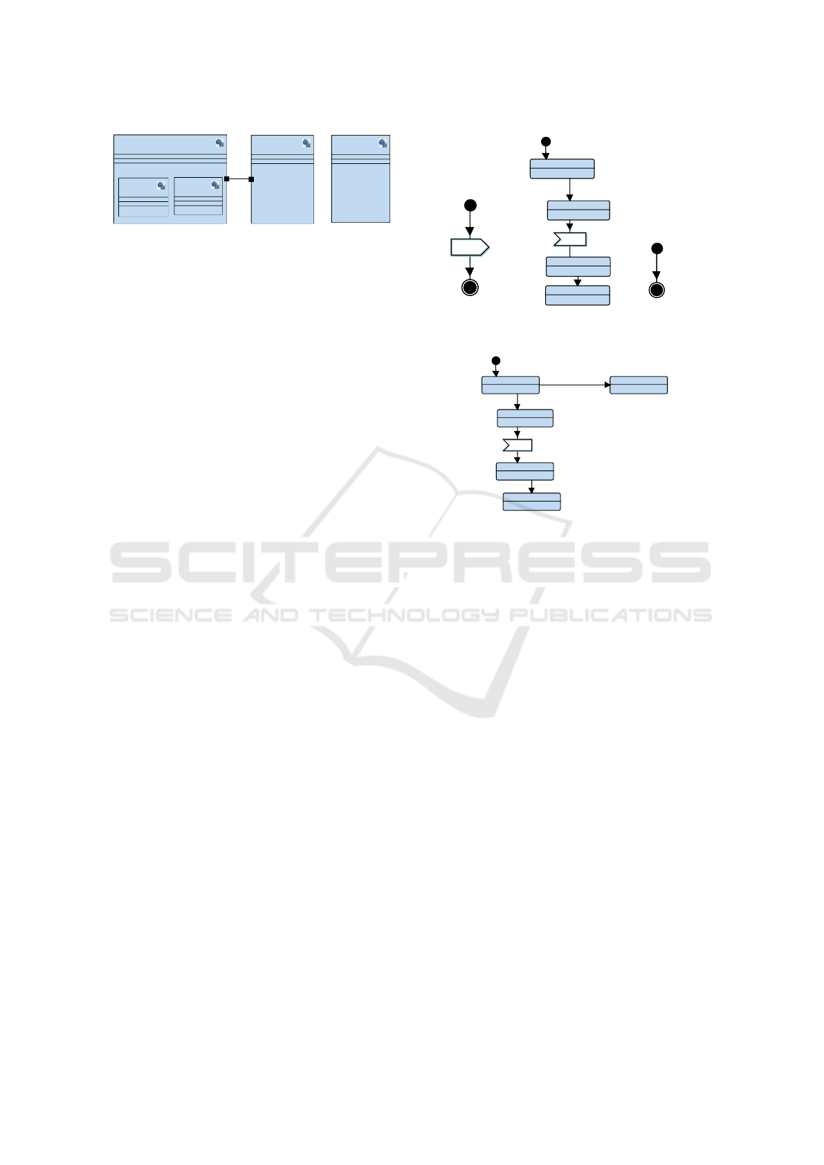
block
Other
Figure 1: Block diagram of the toy system (before muta-
tion).
graph has vertices with no input edges (they corre-
spond to the start states of state machines), vertices
with no output edge (states of state machines with no
output transitions), and other vertices corresponding
to states or transitions.
3.3 Reachability Properties of Mutated
Designs
Since the mutations we study in this paper cannot re-
move existing dependencies (they can also extend the
model, not suppress model elements), the only case
for which a reachability property for an operator o
would not be satisfied anymore is the case where a
new dependency would prevent all dependency paths
to o from being executable. Thus, the main idea is
to compute the new dependencies induced by the mu-
tations, and then to perform a model-checking on a
(hopefully very) reduced system: the one containing
only the new dependencies plus all the first elements
of the dependency paths that necessarily lead to o and
then has no forward mutation. So, if at least one of
them is still reachable, then the reachability property
is still valid on the new system.
Let us illustrate our approach on a toy system.
Since this is a toy system, using this reduction tech-
nique brings only trivial benefits: the idea is not to
illustrate the gain in performance but rather to illus-
trate the principle.
Basically, the toy system has two senders (S1, S2)
that attempt to synchronize via the send signal with
the recv signal of the Receiver block (see Figure 1).
This synchronisation is delayed in the state machines
of senders and receivers with an after clause, as illus-
trated in Figure 2. The Other block does not synchro-
nize with the other blocks: it only waits for a given de-
lay before stopping. As illustrated by the RL in green,
Figure 2, both the reachability and liveness of End1
are satisfied. We use CTL to denote the reachability
of an element: D
I
|= E <> Receiver.End1 means that
the End1 state of the SysML block Receiver is reach-
able in D
I
.
Let us now apply a mutation to this toy system.
We add a new behaviour to Receiver: we add a new
state called End3 and we add a transition from state
send()
after(10)
send()
after(10)
Waiting
recv()
END1
END2
transition
R
R
L
L
after(5)
Waiting
recv()
END1
END2
transition
R
R
L
L
after(5)
after(15)after(15)
Figure 2: State machine diagrams of, from left to right:
S1/S2, Receiver, Other (before mutation).
Waiting
recv()
END1
END2
transition
R
R
L
L
?
?
END3
after(5)
after(2)
Waiting
recv()
END1
END2
transition
R
R
L
L
?
?
END3
after(5)
after(2)
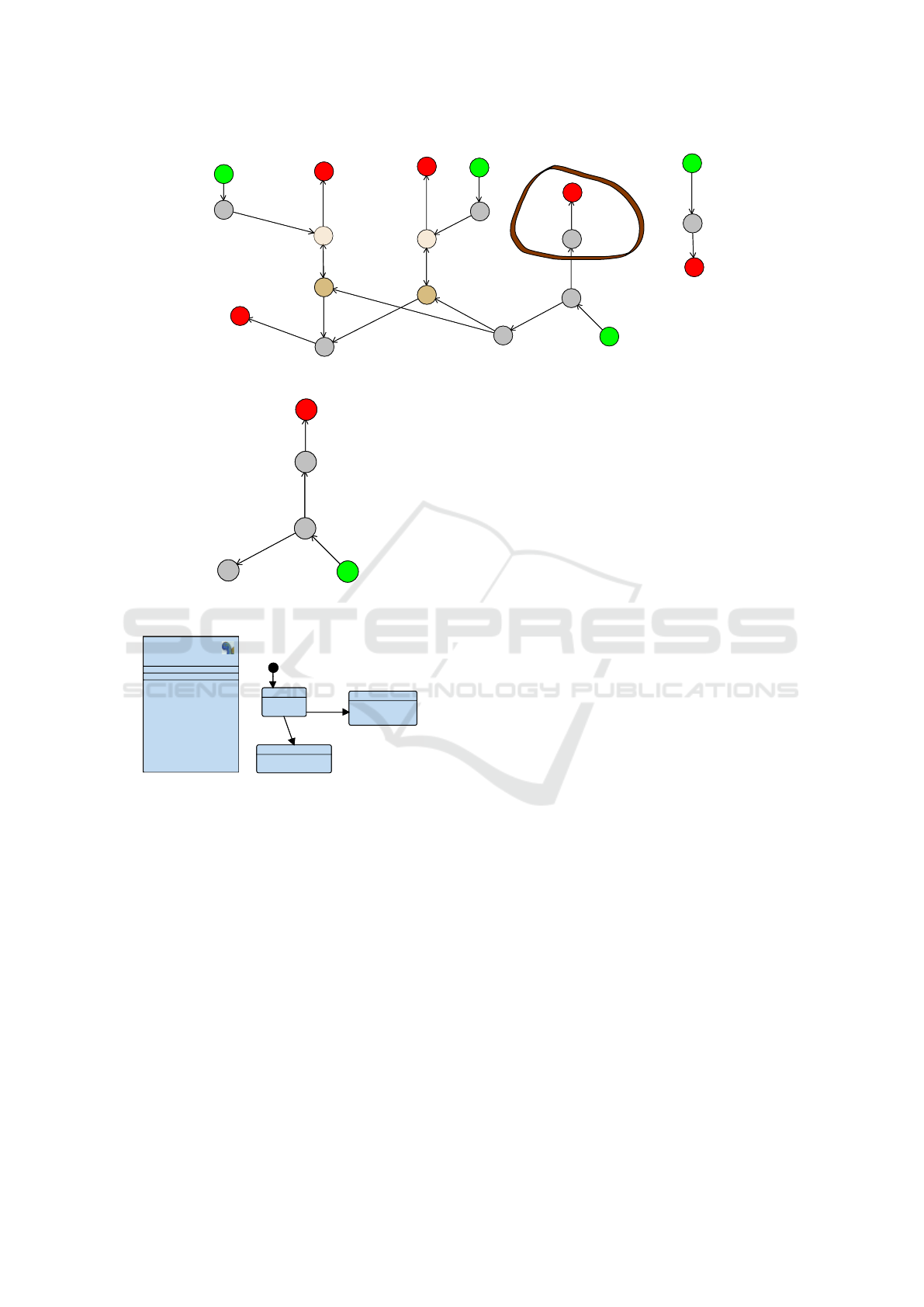
Figure 3: State machine of Receiver (after mutation).
Waiting to state End3 with an after clause after(2)
(Figure 3).
Now, to study if End1 is still reachable after the
mutation, we first need to generate the dependency
graph of the mutated design (Figure 4). This graph
illustrates all logical dependencies of the mutated de-
sign. The green states represent start states of the
state machines. The red states represent end states,
and other states represent other elements (states, tran-
sitions, and sending/receiving actions). The top right
part of the graph represents the Other block. The mid-
dle top part represents the dependencies of S1, while
S2’s dependencies are depicted in the left top part.
Receiver is displayed in the middle and bottom of the
graph. One can notice the two read/write dependen-
cies between S1/Receiver and S2/Receiver leading to
two possible execution paths to reach the End1 state.
We have also rounded in brown the new dependencies
due to the mutation.
Now, let us apply our approach to figure out how
to prove whether the reachability of End1 still holds
after the mutation or not. Since we know that End1
is reachable in D
I
, we know that one of the logi-
cal paths between Receiver/start (i.e., the start state
of the state machine of Receiver 3, displayed as ver-
tex ”3” in the dependency graph) and Receiver/End1
(vertex ”9”) is executable. Let us consider these two
paths, and their intersection with the path from Re-
MODELSWARD 2023 - 11th International Conference on Model-Based Software and Systems Engineering
34
22 / Receiver / Receiving signal "recv"
21 / S1 / Sending signal "send"
20 / Receiver / Receiving signal "recv"
19 / S2 / Sending signal "send"
18 / S1 / stop
17 / S1 / avatar transition
16 / S1 / start
15 / S2 / stop
14 / S2 / avatar transition
13 / S2 / start
10 / Receiver / END2
9 / Receiver / END1
7 / Receiver / avatar transition
6 / Receiver / END3
5 / Receiver / avatar transition
4 / Receiver / Waiting
3 / Receiver / start
2 / Other / stop
1 / Other / avatar transition
0 / Other / start
22 / Receiver / Receiving signal "recv"
21 / S1 / Sending signal "send"
20 / Receiver / Receiving signal "recv"
19 / S2 / Sending signal "send"
18 / S1 / stop
17 / S1 / avatar transition
16 / S1 / start
15 / S2 / stop
14 / S2 / avatar transition
13 / S2 / start
10 / Receiver / END2
9 / Receiver / END1
7 / Receiver / avatar transition
6 / Receiver / END3
5 / Receiver / avatar transition
4 / Receiver / Waiting
3 / Receiver / start
2 / Other /
stop
1 / Other / avatar transition
0 / Other / start
Figure 4: Dependency graph of the design after mutation, before reduction.
7 / Receiver / avatar transition
6 / Receiver / END3
5 / Receiver / avatar transition
4 / Receiver / Waiting
3 / Receiver / start
7 / Receiver / avatar transition
6 / Receiver / END3
5 / Receiver / avatar transitio
n
4 / Receiver / Waiting
3 / Receiver / start
Figure 5: Dependency graph of the design after mutation,
after reduction.
block
Receiver
block
Receiver
Waiting
Transition
R
R
L
L
End3
after(2)
after(5)
Waiting
Transition
R
R
L
L
End3
after(2)
after(5)
Figure 6: Reduced design.
ceiver/End3 to Receiver/state: this intersection is at
state Receiver/Waiting (vertex ”4”). Thus, to know
if End1 is still reachable, we need to know if from
Receiver/Waiting, it is still possible to use one of the
path leading to End1: since these two paths have to
go through vertex 7 first, if vertex 7 is still reachable,
then End1 is still reachable. Otherwise, End1 is not
reachable anymore. So, we can reduce the graph to
all new paths and all paths leading to vertex 7: this
reduced graph is given in Figure 5
From this reduced graph, we can easily recon-
struct a reduced design D
R
(illustrated in Figure 6
from which the reachability of state ‘Transition’ must
now be studied using a model-checker. Obviously,
since the D
R
model is less complex than D
M
, we
expect that studying the reachability of state ‘Tran-
sition’ is much faster than studying the reachability
of state End1 in model D
M
. Since the reachability
of ”Transition” is not satisfied, we can deduce that
D
M
|= E <> Receiver.End1 is false. Finally, the ap-
proach consists in cutting as much as possible the
paths in D
M
that have already been explored when
proving the property in D
I
so as to obtain a reduced
model on which a simplified proof can be performed.
Note that the algorithm does not need to re-display
the reduced SysML model: this is only to better illus-
trate how the model has been cut to reduce the proof
complexity.
3.4 Formalization
Models and dependency graphs are two different rep-
resentations of the same information. Thus in the se-
quel we only consider dependency graphs (denoted
by ”DG”), which abstracts explicit conversions used
in algorithms (i.e., we assume we have Model ≡
graphToModel(modelToGraph(Model))).
Algorithm 1 decides if a set Prop of reachability
properties that have been proved in the initial model
DG
I
are preserved after mutation, i.e. in the mutated
model DG
M
.
For each reachability property p (with associated
vertex v
p
∈ DG
I
), the algorithm first reduces the graph
with reduceGraph, which returns the reduced graph
DG
R
, a new set P
R
of reachability properties to be
proven, and a boolean P which is true if p must be re-
proven on the other returned graph, DG
p
, using paths
to v
p
that are new in DG
M
w.r.t. DG
I
. We first as-
sume that the property is not satisfied anymore. We
then iterate over the set P
R
to see if at least one of
the new reachability properties of P
R
is reachable in
DG
R
, or p in DG
p
. If this is the case, then the set of
mutations DG
I
→ DG
M
preserves p. Otherwise, p is
not preserved.
Algorithm 2 implements the graph reduction. In
this simplified presentation, graphs are handled as sets
containing both vertices and edges. Some explicit
Mutation of Formally Verified SysML Models
35
Algorithm 1: Simplifying reachability proofs after muta-
tion.
Data: DG
I
, DG
M
, Prop
Result: res[Prop]
1 S foreach p ∈ Prop do
2 DG
R
, P
R
, P, DG
p
=
reduceGraph(DG
I
, DG
M
, v
p
)
res(p) = P ∧ prover(DG
p
, p)
3 if not res(p) then
4 foreach p
r
∈ P
R
do
5 result
p
r
= prover(DG
R
, p
r
)
6 if result
p
r
== true then
7 res(p) = true
8 break
9 end
10 end
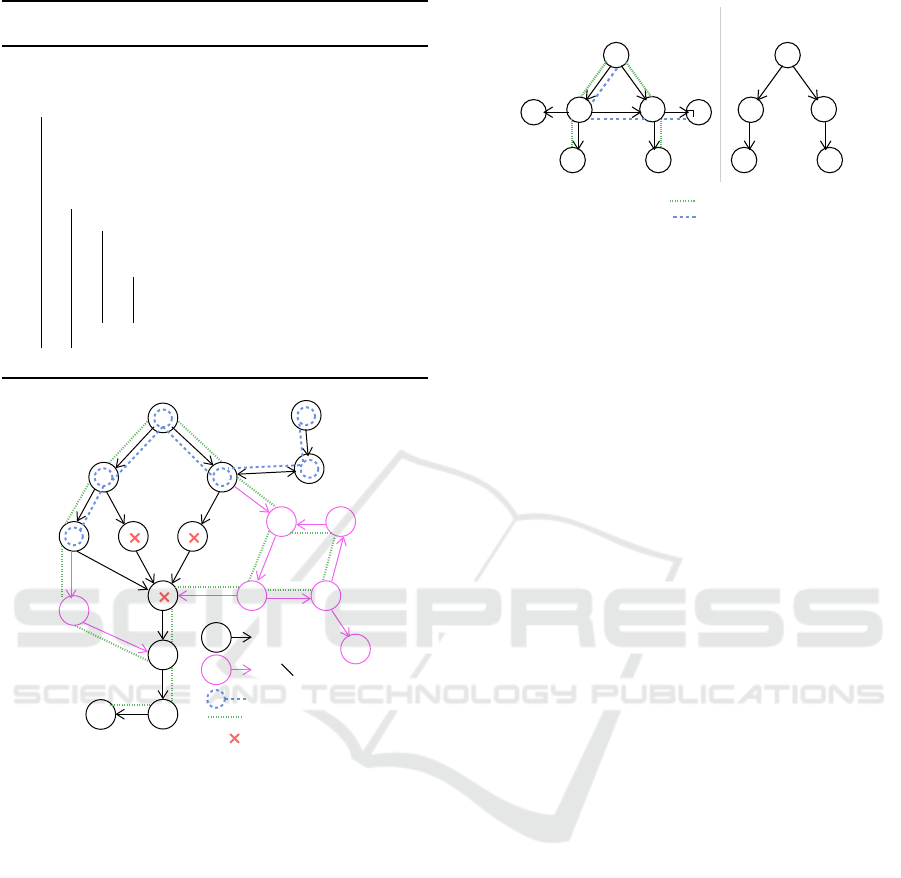
v
p
DG
I
DG
I
DG
M
prefixes
pa
newp
P
R
start start
synchro.
Figure 7: Concepts used in Algorithm 2.
functions and data are not detailed in the scope of this
paper. Figure 7 illustrates some of the corresponding
concepts.
• Paths(DG, V) computes all paths from start ver-
tices of to vertices of V in graph DG.
• v(X) is the set of vertices in Paths(X, v).
• Modified denotes the set of vertices – correspond-
ing to states in state machines – from which a new
transition has been added with mutations.
• addEdges(DG, DG
′
) completes DG with all edges
of DG
′
between vertices common to DG and DG
′
.
• next(V, DG) denotes the set of all direct succes-
sors of any vertex v ∈ V in DG.
• last(w, DG
M
, DG
I
, Modified) is the first vertex in
path w that has no (direct or indirect) successor
v w.r.t. DG
M
verifying v ∈ Modified or v is con-
nected with a vertex of another path of DG
I
that
v
p
v
p
v
p
start
: leading to Vp
: not leading to Vp
runnable paths
runGraph (DG)
v
p
v
p
start
RDG, i.e.
DG
Figure 8: runGraph simplified example.
contains modified nodes: this connection corre-
sponds to a synchronous or asynchronous com-
munication between two blocks that may be com-
promised by mutations.
• prefix(w, DG
M
, DG
I
, Modified) is the prefix of w
that ends at last(w, DG, Modified) (without con-
taining it).
• runGraph(DG,v
p
) (illustrated in Figure 8) is the
Reachable Dependency Graph RDG that only
contains paths of DG that lead from start ver-
tices to v
p
and are ”executable” (i.e. v
p
is actually
reachable w.r.t. these paths).
In Algorithm 2, graphs DG
R
, DG
p
and properties
P
R
are build from empty sets. Vertices are added first,
and edges are added at the end.
1. Lines 1-7. New paths to v
p
in graph DG
M
are
computed (and added to W
newp
): indeed, we need
to evaluate if v
p
could be reachable through these
paths. Thus, if these paths are non empty, they are
added to DG
p
with all the immediate successors
(next) of their vertices. So, only transitions that
may prevent the path to be executed are kept.
2. Lines 8 We compute executable paths able to
reach v
p
in DG
I
.
3. Line 9-15 We then identify the shortest prefixes
(w
pre
) of these paths that cannot lead to any modi-
fied vertices or sensible connection any more. The
idea is that if the remaining suffix (with first ver-
tex v
last
) is reachable then p is reachable, as this
suffix has already been tested on DG
I
. Thus,
we add the reachability of v
last
in P
R
, and the
prefixes (and their ”next”) in DG
R
(lines 12-13).
However, these vertices may also be reachable
from new paths with different values for variables,
which could compromise the execution of the suf-
fix. When such a risk exists (line 14), we require
to re-test the reachability of v
p
and thus add the
prefix to DG
p
(line 15).
4. Line 18-21 We complete both graphs with the ver-
tices of all paths leading to their current vertices:
MODELSWARD 2023 - 11th International Conference on Model-Based Software and Systems Engineering
36
if there is a synchronization needed for a path to
execute, the vertices of the synchronized block
need to be added so that the synchronization can
occur. Finally, we add corresponding edges.
Algorithm 2: Reducing graph to a given reachability prop-
erty p.
Data: DG
I
, DG
M
, v
p
Result: DG
R
, P
R
, P, DG
p
1 DG
R
, P
R
, P, DG
p
= ∅, ∅, false, ∅
2 W
dg
i
= Paths(DG
I
, v
p
)
3 W
dg
m
= Paths(DG
M
, v
p
)
4 W
newp
= W
dg
m
\ W
dg
i
5 if W
newp
̸= ∅ then
6 DG
p
= v(W
newp
) ∪ next(v(W
newp
), DG
M
)
7 P = true
8 W
RDG
I
= Paths(runGraph(DG
I
, v
p
), v
p
)
9 foreach w ∈ W
RDG
I
, v
last
=
last(w, DG
M
, DG
I
, Modified) do
10 w
pre
= prefix(w, DG
M
, DG
I
, Modified)
11 if v
last
̸∈ v(W
newp
) then
12 DG
R
=
DG
R
∪ v(w
pre
) ∪ next(v(w
pre
), DG
M
)
13 P
R
= P
R
S
(E <> v
last
)
14 else
15 DG
p
= DG
p
∪v(w)∪next(v(w), DG
M
)
16 end
17 DG
R
= DG
R
∪ v(Paths(DG
M
, v(DG
R
)))
18 addEdges(DG
R
, DG
M
)
19 DG
p
= DG
p
∪ v(Paths(DG
M
, v(DG
p
)))
20 addEdges(DG
p
, DG
M
)
3.5 Discussion
3.5.1 Optimization
The algorithm has been written to cover all possible
mutations integrated at whatever position in the initial
dependency graph. When there are no mutations on
all paths from the start states to a model element e, the
mutation has no impact on the reachability of e: this
is a property that would be easy to check at first, i.e.,
before our algorithm is run. But again, our algorithm
covers this case, but not in an explicit way and it needs
to compute reachable paths first.
3.5.2 Complexity
The complexity of our algorithm depends on many
factors: the size of the dependency graph, the size
of the reachability graph, the number of paths, the
number of mutations, how mutations impact the de-
pendency graph, and so on. Our approach assumes
that the Dependency Graph (i.e. the model) is much
smaller than the reachability graph of the model.
As a future work, we suggest to evaluate the algo-
rithm, from a performance point of view, as follows:
generate a huge random number of models and of mu-
tations, then randomly select accessibility properties
in these models, and apply our algorithm to these sys-
tems, and finally compute the min, average and max-
imal execution time with regards to the size of the
model and the number of mutations.
Obviously, after too many mutations, or in some
corner cases yet to be defined, directly reproving the
reachability will be faster than applying our algo-
rithm. Indeed, more mutations mean more paths to
compute and evaluate.
3.5.3 Liveness
While this paper focuses on the reachability property,
the liveness of a model element e is another com-
mon property of interest. The liveness of a model
element e is satisfied when all executable paths even-
tually reach v
p
. Without entering into many details
(viz., no definition nor algorithm), we hereafter ex-
plain how liveness could be taken into account in an
incremental way.
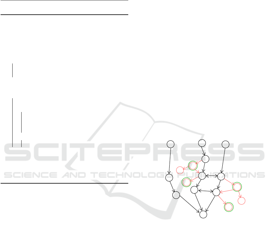
v
p
start
start
start
1
2
3
4
Figure 9: Proving liveness after model mutation.
Figure 9 illustrates the general idea. Basically, we
assume that the prover can output all executable paths
leading to v
p
on the initial model: DG
I
can thus be
reduced to all elements of these paths (black paths in
Figure 9), thus leading to RDG. Let us now assume
that mutations are performed on the initial model, this
leading to a new model DG
M
. New paths in DG
M
that
depend upon at least one element in RDG are added
to RDG (red paths), leading to build a RDG
M
graph.
Black paths such that there are no mutations reaching
them or starting from them can be ignored since their
ability to reach e was examined for DG
I
. On the con-
trary, other paths are to be re-evaluated. For this, we
compute the next elements n (rounded in green on the
figure), of divergent paths (i.e. the first elements of a
red path starting from a black path). Then, for each
Mutation of Formally Verified SysML Models
37

element n, the prover is used, roughly speaking, on
the model reduced to all paths leading to n in DG
M
to figure out if n is reachable or not. If n is reach-
able, then there are two cases. First, if from n there
exists no path to v
p
, then the liveness is not satisfied
anymore. Otherwise, the liveness of v
p
from n must
be evaluated with the prover. For instance, if the next
”2” (Figure 9) is reachable, the the liveness is not sat-
isfied. If the next ”1” is reachable, then the liveness
from ”1” to v
p
must be evaluated. From ”3”, since
there is at least one path leading to v
p
, the liveness to
v
p
must also be evaluated.
Finally, if all reachable next elements n eventually
reach v
p
, then the liveness is satisfied.
4 CASE STUDY
This section illustrates the paper’s contribution in the
scope of a complex case study: an industrial Ethernet-
based Time-Sensitive Networking (TSN).
4.1 Time-Sensitive Networking
Time-Sensitive Networking (TSN) (IEEE, 2018) is
a set of standards defined by IEEE 802.1 Working
Group to provide deterministic services through IEEE
802 Ethernet networks, i.e. guaranteed packet trans-
port with bounded low latency, low packet delay
variation, and low packet loss. Modern embedded
systems and cyber-physical systems, such as safety-
critical industrial, automotive and avionics networks
require deterministic real-time communication.
A TSN network is built upon transmitting End
Systems (Tx ES) sending flows with a given prior-
ity and a period in a network composed of switches
(SW), with a predefined network path for each flow,
and multiple routes handled by frame replication and
elimination. Each end system has a network interface
interconnected with communication switches via full-
duplex physical links (Figure 10). A network path
finishes with one receiving End System (Rx ES). The
network supports unicast and multicast communica-
tions between a set of applications distributed on dif-
ferent end systems.
In the past few years, several research work on
Time-Sensitive networking has relied on model-based
approaches to formally verify properties of the net-
work. In (Guo et al., 2021; Lv et al., 2020), the UP-
PAAL model checker is used for timing analysis of
TSN, while in (Samson et al., 2022; Farzaneh et al.,
2017), network models described in MARTE, respec-
tively EMF, are proposed to serve for automatic gen-
eration of TSN network configurations. By reducing
ES1
ES2
ES3
ES4
SW1
SW3
SW2
SW4
Figure 10: A TSN network architecture.
the verification time of TSN models, the current con-
tribution facilitates the impact of the addition of new
flows or SW in an existing TSN network.
4.2 TSN Model in SysML
In our case study, we propose several TSN network
designs models differing in few mutations (i.e., new
components or behaviours are added from a design
to another) for which we need to verify reachability
properties with the model checker, e.g., the receiving
of a packet is still reachable. These models are in-
tended to be used as a decision helper for dimension-
ing TSN networks for safety-critical applications. We
illustrate different kinds of mutations and show how
our algorithm consider these situations to ease prop-
erty proving.
4.3 TSN Systems, Mutations and
Performance Evaluation
We consider the SysML models of the systems listed
in Table 1. Models contain more than 20 blocks and
complex state machines (the dependency graph con-
tains around 500 vertices corresponding to around 20
blocks and hundred of states and transitions). Per-
formance are given for the system before mutation
and after mutation. After mutation, we show timings
without our approach (no reduction) and with our ap-
proach (with reduction), to indicate the benefits of our
method. The time with reduction includes the time to
generate DG
I
, DG
M
and the proof time for elements
of P, but not the time to compute P nor DG
R
3
. The
performance is computed with the latest version of
TTool (TTool, 2022) (de Saqui-Sannes et al., 2021),
using the internal model-checker of TTool (Calvino
and Apvrille, 2021), and using Oracle Java 11, and
a MacOS laptop with an i7 processor running at 2.3
GHz. For each performance evaluation, we run the
proof 10 times and take the lowest value.
3
Our implementation is not yet complete, but operations
that were not evaluated concern the computation of paths in
dependency graphs, and the latter are of quite small size
with regards to the reachability graphs, as shown in Table 1
MODELSWARD 2023 - 11th International Conference on Model-Based Software and Systems Engineering
38

Table 1: Systems, mutations and performance results.
Reachability Mutation
Proof Proof
States/ Proof States time time DG:
Transi- time Transitions (ms) (ms) vertices/edges/
tions (ms) no red. reduction time to generate
System 1: 1 Tx ES, 2SW, 1 Rx ES, 2 flows
Full reachability
graph generation
1763/3238 16
Adding System 2
(30 blocks)
13k/50k 240126 617/934/5ms
Receiving a
packet in flow 0
- 5 - 227 2
Receiving a
packet in flow 2
- 7 - 231 2
Packet received
in SW#2
- 5 - 232 2
System 2: 2 Tx ES, 3SW, 1 Rx ES, 4 flows
Full reachability
graph generation
80k/200k 292
Adding a flow
sent by Tx ES#1
300k/677k 1170 389/594/2ms
Receiving a
packet in flow 3
- 8 - 11 7
Receiving a
packet in flow 0
- 9 - 10 5
Packet received
in SW#3
- 7 - 10 4
Full reachability
graph generation
Applies to previ-
ous mutation
1.4k/3.4k 4983 395/605/2ms
Receiving a
packet in flow 3
- 8
Adding a flow
sent by Tx ES#2
- 12 4
Receiving a
packet in flow 0
- 9 - 14 4
Packet received
in SW#3
- 7 - 8 4
In the first evaluation, we start from System 1, then
we combine System 1 and System 2 into two indepen-
dent networks. This case is obviously favorable to
our contribution since P contains only the reachabil-
ity of the beginning of the Tx ES blocks since there is
no forward divergence in the dependency graph path.
The proof is therefore straightforward. On the con-
trary, the proof considering the whole system is much
longer. The generation of the dependency graph after
mutation takes around 5 ms and must be done only
once for the three reachability evaluations.
In the second evaluation, we add to System 2 a
new flow. Then, in the third evaluation, we add a sec-
ond mutation to System 2 + previous mutation (also
another flow). In both cases, our approach decreases
the proof time. Also, dependency graphs are of much
smaller size than the reachability graph, which was
part of our assumption for definition of our reduction
algorithm.
In the three investigated mutations, important ad-
ditions have been performed on the model: adding
many blocks in the case of the first mutation, adding
several states and transitions in the case of the second
and third mutations.
As a result, we can conclude that Algorithm 1 de-
creases the proof time for the considered mutations.
Since proving reachability mutations is quite fast, the
gain is not so important but, if we assume that the
reachability shall be proven for all system states, then
the total gain would be much higher. Yet, the ap-
proach is promising and we do hope to apply the same
principle for properties which are much more com-
plex to evaluate, e.g., liveness properties.
5 RELATED WORK
5.1 Formal Verification of SysML
Models
A survey of the literature indicates that formal verifi-
cation has been applied to SysML activity diagrams
(Ouchani et al., 2014; Huang et al., 2019; Staskal
et al., 2022) and state machine diagrams (Delatour
and Paludetto, 1998; Schafer et al., 2001; Apvrille
Mutation of Formally Verified SysML Models
39

et al., 2004), respectively. TTool, which is the SysML
tool considered in the current paper, applies formal
verification to state machine diagrams in the context
of SysML models where each block defining the ar-
chitecture of the system embodies a state machine.
SysML models formal verification tools usually
transform a SysML model into a formal language
that may cater an external and preexisting formal ver-
ification tool. Examples include Petri nets (Dela-
tour and Paludetto, 1998; Szmuc and Szmuc, 2018;
Huang et al., 2019; Rahim et al., 2020), automata for
NuSMV model checker (Wang et al., 2019), timed
automata (Schafer et al., 2001) for UPPAAL model
checker, hybrid automata (Ali, 2018), model checker
NuSMV (Mahani et al., 2021), probabilistic model
checker PRISM (Ouchani et al., 2014; Ali, 2018),
and a theorem prover (Kausch1 et al., 2021). Trans-
lation from UML to process algebra has been in-
vestigated for RT-LOTOS (Apvrille et al., 2004) and
CSP (Ando et al., 2013). The family of correct by
construction specifications has been addressed with
Event B (Bougacha et al., 2022).
The aforementioned papers essentially apply
model checking techniques where a SysML model
is checked against a set of properties. User friend-
liness of formal verification tools therefore depends
on the way properties can be easily expressed or
not. Users of TTool may insert properties inside
the SysML model itself in the form of specific com-
ments (de Saqui-Sannes et al., 2021; Rey de Souza
et al., 2022).
In terms of user friendliness, users of SysML veri-
fication tools are further concerned by verification re-
sults interpretation (Zoor et al., 2021). How to come
back from verification results to the initial state ma-
chines is an issue. It is worth being noticed that the
native model checker of TTool can backtrack verifica-
tion results to the initial SysML model with no obliga-
tion for developers of the SysML diagrams to under-
stand the inner workings of TTool’s model checker.
5.2 Incremental Modeling with SysML
In (Carrillo et al., 2014) Carrillo, Chouali and Moun-
tassir focuses discussion on relationships between re-
quirements and component-based systems architec-
tures. They use Requirement, Sequence and block
diagrams to represent systems requirements, compo-
nents behaviors, and systems architectures, respec-
tively. Atomic requirements are one by one extracted
from the requirement diagrams to incrementally build
an architecture of the system relying on components
libraries. Model checking enables verification of
atomic components modeled in Promela against prop-
erties expressed in the form of LTL formulas.
In (Xie et al., 2022) Xie, Tan, Yang, Li, Xing
and Huang present an integrated SysML modelling
and verification approach where compositional ver-
ification is used to verify the nominal behaviour of
the SysML model and FTA (Fault Tree Analysis) is
used safety analysis. SysML is extended with con-
tract information. SysML models are transformed
into OCRA specifications.
In (Bougacha et al., 2022) Bougacha, Laleau,
Collart-Dutilleul and Ben Ayed translate SysML
models into Event-B specifications, and reuse the re-
finement mechanisms of Event-B to formally verify
the SysML models. The work in (Bougacha et al.,
2022) follows a correct by construction approach.
Conversely, the current paper develops an approach
where each increment in models construction requires
new application of model checking even though the
amount of properties to be verified from an increment
to next one is reduced thanks the mutation principles
presented in the current paper.
5.3 Model Mutation
Alterations of formal models are commonly called
mutations (Von Neumann et al., 1966). Model mu-
tations are particularly used for model-based testing
purposes: for instance, Aichernig et al. (Aichernig
et al., 2013) present a method where a large set of
mutations is applied to a model of a system in order
to detect the implementation mistakes that can inval-
idate the specification of the system. Model muta-
tions can also be used in a security impact assessment
context, since a vulnerability disclosure, an attack or
a countermeasure deployment on a given system can
always be modeled with a mutation of the system’s
model: a vulnerability discovery leads to a change in
the knowledge we have of the system, and an attack
or a countermeasure leads to a change in the system
itself (Sultan et al., 2017). In particular, the W-Sec
method (Sultan et al., 2022) relies on SysML models
for assessing the (positive or negative) impacts of se-
curity countermeasures. The approach introduced in
this paper can therefore help in reducing the complex-
ity of the model-checking stages of testing and impact
assessment methods for SysML models.
6 CONCLUSIONS
(Apvrille et al., 2022) has shown how the perfor-
mance of a SysML model checker can been improved
by computing a dependency graph of the SysML
models before applying model checking to a reduced
MODELSWARD 2023 - 11th International Conference on Model-Based Software and Systems Engineering
40

model. The current paper goes one step forward: it
addresses agility in the context of SysML modeling.
Indeed, the algorithm introduced in the current pa-
per decides how a reachability property proved on a
model before an addition mutation can be proven on
the mutated model without having to consider the en-
tire mutated model. The main principle is to iden-
tify how the new execution paths impact the former
ones. A real-time communication architecture based
on TSN (Time Sensitive Networking) serves as a case
study to illustrate different mutations and shows how
our algorithm performs.
Our vision of future work has already been partly
covered in the discussion subsection. Optimization
is obviously part of our future work to decrease the
complexity: our contribution will increase in interest
when multiple mutations will be take into account.
Handling liveness and more complex properties is
also part of our future work. Also, addressing only
addition mutation can be seen as a limit. Indeed, if
incremental modeling mostly consists in adding new
details, it does not exclude to remove features that are
no longer necessary. Today, our algorithms cannot
handle the removal of modeling elements: this is part
of our future work. Last, the current contribution con-
cerns only safety properties. Yet, performance (Zoor
et al., 2021) and security properties (e.g., confiden-
tiality, integrity, authenticity), as defined in SysML-
Sec (Apvrille and Roudier, 2013), can also be im-
pacted by mutations. We do intend to address these
properties in the future.
REFERENCES
Aichernig, B. K., Lorber, F., and Ni
ˇ
ckovi
´
c, D. (2013).
Time for mutants—model-based mutation testing with
timed automata. In International Conference on Tests
and Proofs, pages 20–38. Springer.
Ali, S. (2018). Formal verification of SysML diagram us-
ing case studies of real-time system. Innovations in
Systems and Software Engineering, 14(6):245–262.
Ando, T., Yatsu, H., Kong, W., Hisazumi, K., and Fukuda,
A. (2013). Formalization and model checking of
SysML state machine diagrams by csp#. In Compu-
tational Science and Its Applications (ICCSA), page
114–127.
Apvrille, L., Courtiat, J.-P., Lohr, C., and de Saqui-Sannes,
P. (2004). TURTLE: A real-time UML profile sup-
ported by a formal validation toolkit. IEEE Transac-
tions on Software Engineering, 30(7):473–487.
Apvrille, L., de Saqui-Sannes, P., Hotescu, O., and Calvino,
A. T. (2022). SysML Models Verification Relying on
Dependency Graphs. In 10th International Confer-
ence on Model-Driven Engineering and Software De-
velopment, Vienna, Austria.
Apvrille, L. and Roudier, Y. (2013). Sysml-sec: A sysml
environment for the design and development of se-
cure embedded systems. In IEEE, editor, APCOSEC
2013, Asia-Pacific Council on Systems Engineering,
September 8-11, 2013, Yokohama, Japan, Yokohama.
© 2013 IEEE. Personal use of this material is permit-
ted. However, permission to reprint/republish this ma-
terial for advertising or promotional purposes or for
creating new collective works for resale or redistri-
bution to servers or lists, or to reuse any copyrighted
component of this work in other works must be ob-
tained from the IEEE.
Bougacha, R., Laleau, R., Collart-Dutilleul, S., and
Ben Ayed, R. (2022). Extending SysML with Re-
finement and Decomposition Mechanisms to Gener-
ate Event-B Specifications. In TASE 2022: Theoreti-
cal Aspects of Software Engineering, volume 13299 of
Lecture Notes in Computer Science, pages 256–273.
Springer.
Calvino, A. T. and Apvrille, L. (2021). Direct model-
checking of SysML models. In Proceedings of the 9th
International Conference on Model-Driven Engineer-
ing and Software Development (Modelsward’2021),
Vienna, Autrichia (online).
Carrillo, O., Chouali, S., and Mountassir, H. (2014). Incre-
mental Modeling of System Architecture Satisfying
SysML Functional Requirements. In Fiadeiro, J. L.,
Liu, Z., and Xue, J., editors, Formal Aspects of Com-
ponent Software (FACS 2013, Lecture Notes in Com-
puter Science, pages 79–99. Springer.
de Saqui-Sannes, P., Apvrille, L., and Vingerhoeds, R. A.
(2021). Checking SysML Models against Safety and
Security Properties. Journal of Aerospace Information
Systems, pages 1–13.
de Saqui-Sannes, P., Vingerhoeds, R. A., Garion, C., and
Thirioux, X. (2022). A taxonomy of MBSE ap-
proaches by languages, tools and methods. IEEE Ac-
cess, 10:120936–120950.
Delatour, J. and Paludetto, M. (1998). UML/PNO: A way
to merge UML and Petri net objects for the analy-
sis of real-time systems. In Oriented Technology:
ECOOP’98 Workshop Reader, page 511–514.
Farzaneh, M. H., Kugele, S., and Knoll, A. (2017). A
graphical modeling tool supporting automated sched-
ule synthesis for time-sensitive networking. In 2017
22nd IEEE International Conference on Emerging
Technologies and Factory Automation (ETFA), pages
1–8. IEEE.
Guo, W., Huang, Y., Shi, J., Hou, Z., and Yang, Y. (2021). A
formal method for evaluating the performance of tsn
traffic shapers using uppaal. In 2021 IEEE 46th Con-
ference on Local Computer Networks (LCN), pages
241–248. IEEE.
Huang, E., McGinnis, L., and Mitchell, S. (2019). Verifying
sysml activity diagrams using formal transformation
to Petri nets. Systems Engineering, 23(1):118–135.
IEEE (2018). 802.1Q - IEEE Standard for Local and
Metropolitan Area Networks—Bridges and Bridged
Networks. ” https://standards.ieee.org/ standard/802
1Q-2018.html.
Mutation of Formally Verified SysML Models
41

Kausch1, M., Pfeiffer1, Raco1, D., and Rumpe, B. (2021).
Model-based design of correct safety-critical systems
using dataflow languages on the example of SysML
architecture and behavior diagrams. In AVIOSE’2021,
Software Engineering 2021 Satellite Events, Bonn,
Germany (virtual), Lecture Notes in Informatics
(LNI), Gesellschaft f
¨
ur Informatik, pages 1–22.
Lv, J., Zhao, Y., Wu, X., Li, Y., and Wang, Q. (2020).
Formal analysis of tsn scheduler for real-time com-
munications. IEEE Transactions on Reliability,
70(3):1286–1294.
Mahani, M., Rizzo, D., Paredis, C., and Wang, Y. (2021).
Automatic formal verification of SysML state ma-
chine diagrams for vehicular control system. SAE
Technical Paper.
OMG (2017). OMG Systems Modeling Lan-
guage. Object Management Group,
https://www.omg.org/spec/SysML/1.5.
Ouchani, S., Ait Mohamed, O., and Debbabi, M. (2014).
A formal verification framework for SysML activity
diagrams. Expert Systems with Applications, 41(6).
Rahim, M., Boukala-Loualalen, M., and Hammad, A.
(2020). Hierarchical colored Petri nets for the veri-
fication of SysML designs - activity-based slicing ap-
proach. In 4th Conf. on Computing Systems and Appli.
(CSA 2020), volume 199 of Lecture Notes in Networks
and Systems, pages 131–142, Algiers, Algeria.
Rey de Souza, F. G., Hirata, C. M., and Nadjm-Tehrani, S.
(2022). Synthesis of a controller algorithm for safety-
critical systems. IEEE Access, 10:76351–76375.
Samson, M., Vergnaud, T., Dujardin,
´
E., Ciarletta, L., and
Song, Y.-Q. (2022). A model-based approach to auto-
matic generation of tsn network simulations. In 2022
IEEE 18th International Conference on Factory Com-
munication Systems (WFCS), pages 1–8. IEEE.
Schafer, T., Knapp, A., and Merz, S. (2001). Model
checking UML state machines and collaborations.
Electronic Notes in Theoretical Computer Science,
55:357–369.
Staskal, O., Simac, J., Swayne, L., and Rozier, K. Y. (2022).
Translating sysml activity diagrams for nuxmv verifi-
cation of an autonomous pancreas. In SESS22), pages
1–6.
Sultan., B., Apvrille., L., and Jaillon., P. (2022). Safety, se-
curity and performance assessment of security coun-
termeasures with sysml-sec. In Proceedings of
the 10th International Conference on Model-Driven
Engineering and Software Development - MODEL-
SWARD,, pages 48–60. INSTICC, SciTePress.
Sultan, B., Apvrille, L., and Jaillon, P. (2022). Safety, secu-
rity and performance assessment of security counter-
measures with sysml-sec. In 10th International Con-
ference on Model-Driven Engineering and Software
Development.
Sultan, B., Dagnat, F., and Fontaine, C. (2017). A method-
ology to assess vulnerabilities and countermeasures
impact on the missions of a naval system. In Com-
puter Security, pages 63–76. Springer.
Szmuc, W. and Szmuc, T. (2018). Towards embedded sys-
tems formal verification translation from SysML into
Petri nets. In 25th International Conference Mixed
Design of Integrated Circuits and System (MIXDES),
pages 420–423.
TTool (2022). https://ttool.telecom-paris.fr/. Retrieved May
11, 2022.
Von Neumann, J., Burks, A. W., et al. (1966). Theory
of self-reproducing automata. IEEE Transactions on
Neural Networks, 5(1):3–14.
Wang, H., Zhong, D., Zhao, T., and Ren, F. (2019). Inte-
grating model checking with sysml in complex system
safety analysis. IEEE Access, 7:16561–16571.
Xie, J., Tan, W., Yang, Z., Li, S., Xing, L., and Huang, Z.
(2022). Sysml-based compositional verification and
safety analysis for safety-critical cyber-physical sys-
tems. Connection Science, 34(1):911–941.
Zoor, M., Apvrille, L., and Pacalet, R. (2021). Execu-
tion Trace Analysis for a Precise Understanding of
Latency Violations. In International Conference on
Model Driven Engineering Languages and Systems
(MODELS), Fukuoka (virtual), Japan.
MODELSWARD 2023 - 11th International Conference on Model-Based Software and Systems Engineering
42
