Multi-Objective Deep Q-Networks for Domestic Hot Water Systems
Control
Mohamed-Harith Ibrahim
1,2
, St
´
ephane Lecoeuche
1
, Jacques Boonaert
1
and Mireille Batton-Hubert
2
1
IMT Nord Europe, Institut Mines-T
´
el
´
ecom, Univ. Lille, Centre for Digital Systems, F-59000 Lille, France
2
Mines Saint-Etienne, Univ Clermont Auvergne, CNRS, UMR 6158 LIMOS,
Institut Henri Fayol, F-42023, Saint Etienne, France
Keywords:
Multi-Objective Reinforcement Learning, Deep Reinforcement Learning, Electric Water Heater.
Abstract:
Real-world decision problems, such as Domestic Hot Water (DHW) production, require the consideration of
multiple, possibly conflicting objectives. This work suggests an adaptation of Deep Q-Networks (DQN) to
solve multi-objective sequential decision problems using scalarization functions. The adaptation was applied
to train multiple agents to control DHW systems in order to find possible trade-offs between comfort and
energy cost reduction. Results have shown the possibility of finding multiple policies to meet preferences of
different users. Trained agents were tested to ensure hot water production with variable energy prices (peak
and off-peak tariffs) for several consumption patterns and they can reduce energy cost from 10.24 % without
real impact on users’ comfort and up to 18 % with slight impact on comfort.
1 INTRODUCTION
Different methods and techniques are used to con-
trol DHW systems. Optimization based methods and
Reinforcement Learning (RL) are the most studied
approaches in literature to adapt operations of sys-
tems to real needs. Authors in (Kapsalis et al., 2018)
present an optimization based method to schedule the
operation of an Electric Water Heater (EWH) for a
given hot water consumption pattern under dynamic
pricing and takes into account cost and comfort of
users. In (Shen et al., 2021), authors propose an MPC-
based controller to minimize electricity cost while
maintaining comfort under uncertain hot water de-
mand and peak/off-peak rate periods. MPC is an opti-
mization based method that consists of modelling the
system to be controlled, predicting its future behav-
iors and disturbances and controlling by taking ac-
tions that satisfy constraints and optimize desired ob-
jectives. The major drawback of optimization based
approach is in the necessity of having a precise dy-
namic model of the system. Problems can arise be-
cause of the non adaptive nature of the model which
can lead to sub-optimal performances.
On the other hand, multiple studies use RL to con-
trol DHW systems (Heidari et al., 2022) (Amasyali
et al., 2021) (Ruelens et al., 2016) (Patyn et al., 2018)
(Kazmi et al., 2018). In (Amasyali et al., 2021), au-
thors train different agents using DQN to minimize
electricity cost of water heater without causing dis-
comfort to users. Their results are compared to other
control methods and their approach outperforms rule-
based methods and MPC based controllers. In (Hei-
dari et al., 2022), authors suggest to use Double DQN
to balance comfort, energy use and hygiene in DHW
systems. The agent learns stochastic occupants’ be-
haviors in an offline training procedure integrating a
stochastic hot water model to mimic the use of occu-
pants. The balance between these objectives is based
on the design of the reward function which returns a
single reward value.
To the best of author’s knowledge, the existing
works about DHW production control do not con-
sider the conflicting nature of the studied objectives.
For many decision problems that require the consid-
eration of an important number of objectives, the in-
creasing of performances of one objective may de-
crease the performances of other objectives. In ad-
dition, preferences over objectives can be expressed
in multiple ways and may be different depending on
users that are affected by the decision process.
Multi-Objective Reinforcement Learning
(MORL) extends RL to problems with two or
more objectives. Multiple studies adapt existing
single-objective methods to a multi-objective context.
Authors in (Van Moffaert et al., 2013) propose a
234
Ibrahim, M., Lecoeuche, S., Boonaert, J. and Batton-Hubert, M.
Multi-Objective Deep Q-Networks for Domestic Hot Water Systems Control.
DOI: 10.5220/0011647400003393
In Proceedings of the 15th International Conference on Agents and Artificial Intelligence (ICAART 2023) - Volume 3, pages 234-242
ISBN: 978-989-758-623-1; ISSN: 2184-433X
Copyright
c
 2023 by SCITEPRESS – Science and Technology Publications, Lda. Under CC license (CC BY-NC-ND 4.0)

general framework to adapt Q-learning to a multi-
objective problems using a scalarization function
that expresses preferences over different objectives.
This can be done in a case of a prior articulation of
preferences over objectives.
Some real-world problems are complex and may
require the use of value function approximation to
scale up tabular methods. DQN was presented in
(Mnih et al., 2015) for single-objective cases. In
this paper, we focus on solving multi-objective se-
quential decision problems by learning a single pol-
icy in a known preferences scenario with value-based
methods. This is done by adapting DQN to solve
multi-objective problems using scalarization func-
tions. This method is used to train a controller to take
decisions about DHW production. Its objectives are
to maximize comfort and to minimize energy cost.
The reminder of the paper is structured as follows.
Section 2 gives a brief introduction to MORL. In Sec-
tion 3, we present an adaptation of DQN to multi-
objective problems. The control of DHW production
and the experimental setup are presented in Sections
4 and 5. Finally, results for DHW production control
are given in Section 6.
2 MULTI-OBJECTIVE
REINFORCEMENT LEARNING
2.1 Definition
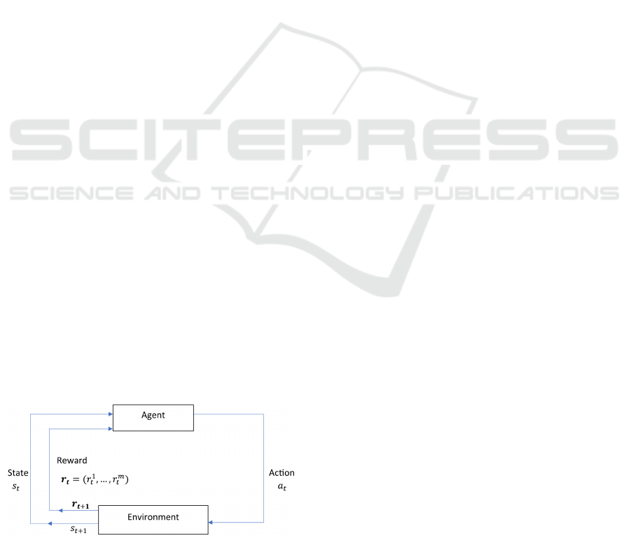
MORL can be viewed as the combination of
multi-objective optimization and RL to solve multi-
objective sequential decision problems. It is a branch
of RL that involves multiple, possibly conflicting ob-
jectives. As illustrated in Fig. 1, at each time step t,
the agent, in a certain state s
t
, interacts with its envi-
ronment via an action a
t
that changes its state to s
t+1
and provides a reward vector r
t+1
containing a reward
element for each objective. The reward function is a
vector function that describes a vector of m rewards
instead of a scalar.
Figure 1: Agent-environment interaction in a multi-
objective decision process.
Due to the vector reward function, state-value
function V and action-value function Q under policy
π are replaced by vector value functions V
π
and Q
π
:
V
π
(s) = (V
(1)
π
(s),...,V
(m)
π
(s)), (1)
Q
π
(s,a) = (Q
(1)
π
(s,a), ...,Q
(m)
π
(s,a)), (2)
where
V
(i)
π
(s) = E
π
[
T
∑
n=0
γ
n
r
(i)
t+n+1
|s
t
= s], (3)
and
Q
(i)
π
(s,a) = E
π
[
T
∑
n=0
γ
n
r
(i)
t+n+1
|s
t
= s, a
t
= a], (4)
where T is the size of the sequence, m is the number
of objectives, γ is the discount factor which is used
to quantify the importance of short-term versus long-
term rewards and r
(i)
is the reward for objective i.
The main goal for an agent in MORL problems is
to optimize its expected cumulative rewards by learn-
ing a policy that best maps between states and actions.
2.2 Optimality in Multi-Objective
Decision Problems
In multi-objective decision problems, no single pol-
icy exists that optimizes simultaneously all conflict-
ing objectives. Instead, there exist a set of policies
and one has to be chosen in the presence of trade-
off between objectives. Therefore, to compare differ-
ent policies and to define optimality in multi-objective
problems, we use Pareto dominance relation as it was
done in (Van Moffaert, 2016).
A policy π weakly Pareto dominates another pol-
icy π
0
when there does not exist an objective i where
π
0
is better than π over all states:
π  π
0
⇐⇒ ∀i,V
(i)
π
(s) ≥ V
(i)
π
0
(s). (5)
Two policies are incomparable if some objectives
have lower values for the first policy while others have
higher values for the second policy and vice versa. Fi-
nally, a policy π is Pareto optimal if it either Pareto
dominates or is incomparable to all other policies.
Multiple Pareto optimal policies could exist and
the choice of a policy depends on the importance
given to each objective. The set of Pareto optimal
policies is called Pareto front.
Multi-Objective Deep Q-Networks for Domestic Hot Water Systems Control
235

2.3 Preferences over Objectives
Authors in (Liu et al., 2014) give a detailed overview
of several MORL approaches. One way to express in-
formation about prioritizing objectives is to scalarize
the multi-objective problem. Scalarizing means for-
mulating a single-objective problem such that optimal
policies to the single-objective problem are Pareto op-
timal policies to the multi-objective problem (Hwang
and Masud, 2012). In addition, with different param-
eters quantifying the importance of each objective for
the scalarization, different Pareto optimal policies are
produced. Scalarizing in MORL means applying a
scalarization function f and a weight vector w to the
Q-vector that contains Q-values of all objectives. This
is done in the action selection stage in order to opti-
mize the scalarized value expressed as follows:
SQ(s, a) = f (Q(s, a), w). (6)
The scalarization function can be a linear scalar-
ization function that computes a weighted sum of all
Q-values. Other scalarization functions like Cheby-
shev scalarization (Van Moffaert et al., 2013) are
also used in MORL. Besides, non-linear methods like
Threshold Lexicographic Q-Learning (TLQ) (Vam-
plew et al., 2011) were proposed to learn a sin-
gle policy in MORL. Nevertheless, some approaches
may converge to a sub-optimal policy or even fail
to converge in certain conditions as it was shown
in (Issabekov and Vamplew, 2012) for TLQ. In fact,
temporal-difference methods based on Bellman equa-
tion are incompatible with non-linear scalarization
functions due to the non-additive nature of the scalar-
ized returns (Roijers et al., 2013). Therefore, in what
follows, we consider f as a linear scalarization func-
tion and w a weight vector such as:
f (Q(s,a), w) =
m
∑
i=1
w
i
Q
(i)
(s,a), (7)
where ∀i,0 ≤ w
i
≤ 1 and
∑
m
i=1
w
i
= 1.
2.4 Action Selection in MORL
In value based RL methods, the optimal policy is de-
rived from estimated Q-values by selecting actions
with the highest expected cumulative rewards: we
choose greedy actions.
a = argmax
a
0
Q(s,a
0
). (8)
In MORL, the Pareto optimal policy is derived
from estimated Q-vectors by selecting actions with
the highest scalarized expected cumulative rewards:
we choose scalarized greedy actions.
a = argmax
a
0
SQ(s, a
0
). (9)
In order to balance exploration and exploitation,
we use ε-greedy action selection. ε refers to the prob-
ability of choosing to explore by selecting random
actions while 1 − ε is the probability of exploiting
by taking advantage of prior knowledge and selecting
greedy actions.
3 MULTI-OBJECTIVE DEEP
Q-NETWORKS
It is important to recall that DQN is about training a
Neural Network (NN) with parameters θ to approxi-
mate the action-value function of the optimal policy
π
∗
.
Q
θ
(s,a) ≈ Q
π
∗
(s,a) = E
π
∗
[
T
∑
n=0
γ
n
r
t+n+1
|s
t
= s, a
t
= a].
(10)
The NN takes a state as an input and outputs the value
of each possible action from that state. The method is
characterized by:
• The use of a replay memory to store experiences.
• The use of two networks: a policy network Q
θ
and a target network Q
θ
0
. The policy network
determines the action to take and is updated fre-
quently by training on random batches from the
replay memory. The target network is an old ver-
sion of the policy network and is updated copying
its weights from the policy network at regular in-
tervals. It is used to compute targets Q(s, a) noted
y as follows:
y = r + γmax
a
0
Q
θ
0
(s
0
,a
0
). (11)
The target is the estimated value of a state-action
pair (s, a) under the optimal policy. It is the sum of the
immediate reward r received after taking action a in
state s and the estimated discounted maximum value
from next state s
0
.
In this section we adapt DQN to multi-objective
sequential decision problems. We suggest to train an
NN Q
θ
with parameters θ to approximate the action-
value vector function Q of an optimal policy. The NN
takes a state as an input and it outputs the value of
each possible action for each objective from that state.
The argument of separating Q-values for each objec-
tive instead of learning one scalarized Q-value is that
values of individual objectives may be easier to learn
than the scalarized one, particularly when function
approximation is employed as mentioned in (Tesauro
et al., 2007).
Similarly to DQN, we use a target network Q
θ
0
of
parameters θ
0
to compute the targets. However, mul-
tiple changes are made to DQN:
ICAART 2023 - 15th International Conference on Agents and Artificial Intelligence
236

.
.
.
.
.
.
.
.
.
.
.
.
Q
1
(s, a
1
)
Q
1
(s, a
2
)
Q
m
(s, a
n
)
State
Hidden layer Hidden layer
Output
layer
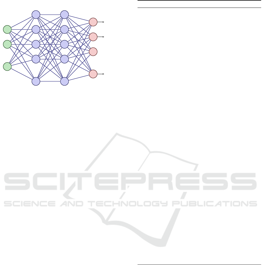
Figure 2: Architecture of a neural network to estimate Q-
values for m objectives.
• The output layer of the trained NN outputs the
value of each possible action for each objective.
The size of the output layer becomes n × m where
n is the number of possible actions at each time
step (see Fig. 2).
• Action selection: the scalarization function f and
the weight vector w are involved in the action se-
lection process to express the importance of each
objective. The greedy action becomes the action
that guarantees the highest scalarized action-value
as explained in Subsection 2.4.
• Replay memory: for each experience e, we store
a reward vector r that contains a reward value
for each objective. These experiences are used to
train the value network.
e = (s, a, r, s
0
). (12)
• Target value computation is done for each objec-
tive i. The target is the sum of the immediate re-
ward of the i’th objective and the i’th component
of the Q vector of the scalarized greedy action a
0
from next state s
0
using the target network:
y
(i)
= r
(i)
+ γQ
(i)
θ
0
(s
0
,a
0
). (13)
• The value network is trained to minimize the
mean squared temporal difference error for each
objective:
L(θ) =
m
∑
i=1
E[(y
(i)
− Q
(i)
θ
(s,a))
2
]. (14)
In whats follows, we note y as the vector of target
values for each objective.
Multi-Objective DQN (MO-DQN) is a single pol-
icy method that requires prior knowledge of prefer-
ences over different objectives. The method is sum-
marized in Algorithm 1.
Algorithm 1: Multi-Objective DQN.
1: Initialize replay memory D to capacity N
2: Choose number of episodes M and episode length
T
3: Choose learning rate α, discount factor γ and
batch size B
4: Choose scalarization function f and weight vec-
tor w
5: Initialize value network Q
θ
with random weights
θ
6: Copy the value network to create the target net-
work Q
θ
0
7: for episode=1, M do
8: Get an initial state
9: for t = 1, T do
10: With probability ε select random action a
t
11: Otherwise a
t
= argmax
a
f (Q
θ
(s
t
,a), w)
12: Execute action a
t
and get rewards r
t+1
and next state s
t+1
13: Store experience (s
t
,a
t
,r
t+1
,s
t+1
) in D
14: Move to next state s
t+1
15: Sample a random batch D
B
of size B of
experiences from D every T
train
steps
16: for each experience (s,a, r,s
0
) ∈ D
B
do
17: Calculate Q
θ
0
(s
0
,a
0
) the Q vector of
the scalarized greedy action a
0
from the next state
s
0
using the target network Q
θ
0
18: Calculate expected state-action pair
(s,a) values
y = r + γQ
θ
0
(s
0
,a
0
)
19: end for
20: Train value network Q
θ
on D
B
to mini-
mize the loss function expressed in Equation (14)
21: end for
22: Update ε for exploration probability
23: Update target network’s weights θ
0
with the
weights of the value network every K step
24: end for
4 DOMESTIC HOT WATER
PRODUCTION PLANNING AND
CONTROL
In this section, we study the control of an EWH. The
goal is to train a controller using MO-DQN to take
decisions about DHW production considering users’
comfort and energy cost. Preferences over these two
objectives may be different from householder to an-
other. In addition, increasing comfort may increase
energy cost. Thus, decision-making in this case is
about finding a trade-off between conflicting objec-
Multi-Objective Deep Q-Networks for Domestic Hot Water Systems Control
237

tives based on preferences over objectives.
The controller has to take a decision about water
heating for the next time step based on information
at current time step. In addition, the decision process
considers importance given to each objective using a
scalarization function f and a weight vector w.
4.1 State Representation
The state vector s
t
is a representation of the environ-
ment at time t. It contains time-related components,
such as hour of the day h and day of the week d, tem-
perature measurement T , DHW consumption V
DHW
and electricity tariff λ:
s
t
= (h(t),d(t), T (t),V
DHW
(t), λ(t)), (15)
s
t
∈ S where S is the state space.
The time-related information helps the agent to as-
sociate repeated behaviors to time without requiring
prediction of DHW consumption. In fact, as shown
in (Heidari et al., 2021), hot water use behaviors are
highly correlated with the same time of the day and
the behaviors during the weekdays can be similar and
different from the weekends.
For energy cost, we use french electricity tariffs in
early 2022 with two periods : off-peak time and peak
time. The price of 1 kWh is in euro and is 25.1% more
expensive in peak time:
λ =

0.147 from 12 am to 8 am,
0.184 from 9 am to 11 pm.
(16)
4.2 Control Actions
At each time step t, the agent takes an action a
t
∈ A
where A = {0,20, 40, 60} is the action space. The ac-
tion is taken each hour (∆t = 60 minutes) based on the
current state and it represents the duration, in minutes,
of production at time step t. We assume that the EWH
has a rated power P
elec
of 2.2 kW.
4.3 Reward Shaping
To minimize energy cost, we design a cost reward
where the agent is penalized each time it decides to
produce DHW. The reward takes into consideration
the duration of production and electricity tariff. This
would encourage the agent to shift DHW to periods
where energy is less expensive and to reduce its en-
ergy consumption by reducing the duration of DHW
production. The received reward after a decision a
t
at
state s
t
for energy cost is:
r
cost
t+1
= −
a
t
∆t
× P
elec
× λ(t). (17)
In order to avoid discomfort situations, we design
a comfort reward where the agent is penalized each
time the temperature of DHW is lower than a mini-
mum threshold accepted by the user called T
pre f
. This
would motivate the agent to stay in a state where water
temperature is acceptable for the user. The received
reward after a decision a
t
at state s
t
for comfort is:
r
com f ort
t+1
=

0 if T (t + 1) ≥ T
pre f
,
−10 otherwise.
(18)
Both rewards are normalized to have a common
scale. The importance of each objective is expressed
using the scalarization function f in the action selec-
tion process. Thus, the reward function R is defined
as follow:
R : S × A × S → R
2
(19)
(s,a, s
0
) 7−−→(r
com f ort
,r
cost
).
5 EXPERIMENTAL SETUP
5.1 Environment
To train an agent, we create a virtual environment
composed of two parts. The first part simulates the be-
havior of a DHW system. We consider an EWH com-
posed of a water buffer of 200 liters and an electrical
heating element. When there is a DHW consumption,
the hot water is drawn from the buffer and replaced
by the same amount of cold water. We model the ther-
mal dynamics with a one-node model as it was done
in (Shen et al., 2021). It assumes that water inside the
tank is at a single uniform average temperature. The
modelling takes into consideration:
• Heat loss from water to its ambient environment
that depends on thermal resistance and dimen-
sions of the tank.
• Heat loss due to water demand that depends on
the volume of consumed water and on cold wa-
ter temperature that replaces hot water inside the
tank.
• Heat injected inside the tank which depends on
the available power to heat the water.
The second part of the environment simulates
users’ behaviors. We simulate DHW data using (Hen-
dron et al., 2010). The idea is to train an agent on a
high number of different DHW consumption scenar-
ios. This can help the agent to extract repeated be-
haviors, identify probable consumption periods and
to adapt hot water production to real needs.
ICAART 2023 - 15th International Conference on Agents and Artificial Intelligence
238

It should be noted that the agent has no access to
the described environment. In fact, the modelling is
done to create an environment to train the agent and
to compute agent’s state at each time step.
5.2 Agent Setup
We choose to train a fully connected NN to estimate
the action-value vector function with MO-DQN. The
size of the output layer of the NN is eight (two ob-
jectives and four actions). To test different configura-
tions, we train multiple agents with different prefer-
ences over objectives using multiple weight vectors
w. Each vector contains, in the following order, a
weight for comfort and a weight for energy cost.
Hyperparameters of the NN and the agent were
tuned and are shown in Table 1.
Table 1: Hyperparameters of MORL agent training.
Parameter Value
Memory size (N) One year
Number of episodes (M) 1000
Episode length (T ) One day
Scalarization function Linear scalarization
Exploration Linear decay
Update frequency (K) Five episodes
Discount factor (γ) 0.95
Number of hidden layers 2
Activation function Leaky ReLU
Number of nodes 128
Batch size (B) 32
Learning rate (α) 0.0001
5.3 Evaluation Approach
To evaluate the performance of the described method
in Section 3 on DHW production problem, we com-
pare it to a conventional rule-based control method.
The rule-based method switches hot water production
on whenever water temperature is below a threshold
T
min
and is stops when temperature exceeds an upper
threshold T
max
.
We choose to compare multiple MO-DQN agents
with different preferences over objectives to rule-
based method with different thresholds:
• T
max
= 65
◦
C and T
min
= 62
◦
C (baseline).
• T
max
= 60
◦
C and T
min
= 57
◦
C.
• T
max
= 55
◦
C and T
min
= 52
◦
C.
Performances are compared on comfort and on en-
ergy cost reduction as these are the initial objectives
to optimize. Comfort is defined as the proportion of
time with a temperature greater or equal than T
pre f
while energy cost reduction is the reduction of cost
compared to the baseline. For safety issues, DHW
production stops automatically when water tempera-
ture is above 65
◦
C for all control methods.
Both rule-based method and MO-DQN are tested
and used to produce DHW for unseen consumption
data during twelve weeks. The DHW consump-
tion comes from five different domestic water heaters
which were measured and made available by (Booy-
sen et al., 2019)
6 RESULTS AND DISCUSSION
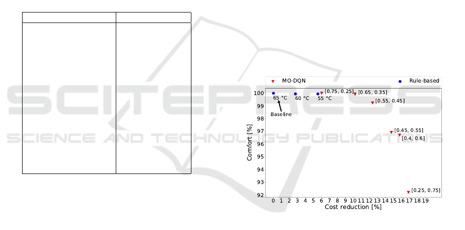
Figure 3 shows average results on comfort and en-
ergy cost reduction using MO-DQN and rule based
method. It appears that minimizing energy cost and
maximizing comfort are two conflicting objectives,
since maximizing one leads to minimizing the other.
In addition, no agent outperforms other agents over
both objectives. In other words, all policies learned
by agents are incomparable and could be a part of the
Pareto front.
Figure 3: Average results obtained on comfort and energy
cost using MO-DQN agents and rule-based method.
Results also show that MO-DQN agents outper-
form rule-based method with any chosen threshold in
terms of cost reduction. Agents offer multiple possi-
ble trade-offs between comfort and energy cost. For
example, a cautious policy can reduce energy cost
up to 10.82% (10.42% on average) without any real
impact on comfort (99.9 % on average) when w =
[0.65,0.35]. Other less cautious policies can reach
18% of energy cost reduction on some consumption
profiles with a slight impact on comfort.
Table 2 details how agents reduce energy cost ac-
cording to preferences and focuses on the impact of
agents’ behaviors on discomfort. Unlike comfort (see
definition in Subsection 5.3), discomfort measures the
Multi-Objective Deep Q-Networks for Domestic Hot Water Systems Control
239

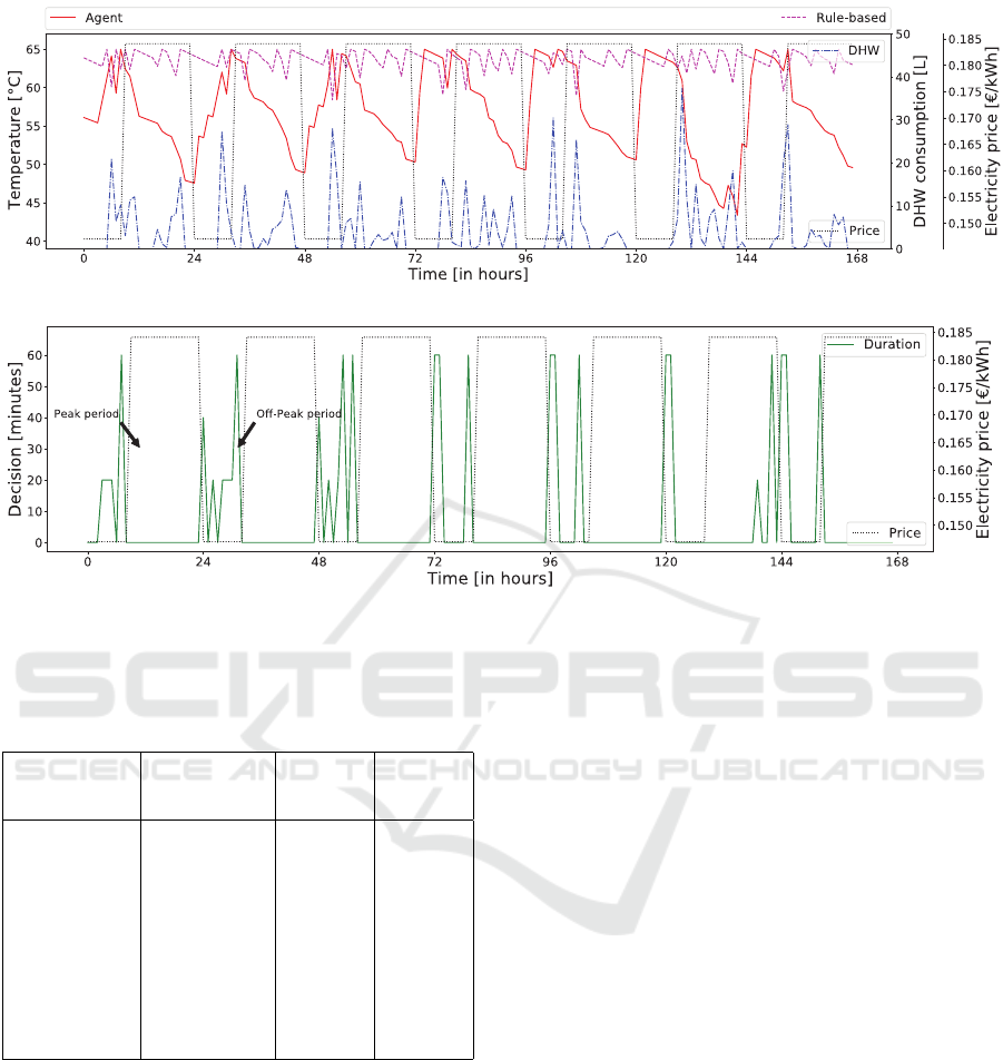
(a) Temperature profiles in terms of electricity prices and DHW consumption.
(b) MO-DQN agent decisions in terms of electricity prices.
Figure 4: Comparison of DHW production between rule-based method and MO-DQN during one week with w = [0.45, 0.55].
Table 2: Comparison between different agents to control
DHW production. Shown scores are averages obtained on
five consumption profiles.
Method Discomfort Energy
saving
(%)
Off-peak
actions
(%)
Baseline (65
◦
C) (0, -) - -
w = [0.75,0.25] (0, -) 2.03 40.76
w = [0.65,0.35] (1, 38.85
◦
C) 3.52 57.21
w = [0.55,0.45] (8, 37.61
◦
C) 7.35 68.46
w = [0.45,0.55] (27.2, 37.73
◦
C) 7.1 72.65
w = [0.4,0.6] (40, 37.65
◦
C) 7.78 79.88
w = [0.25,0.75] (99.4, 37.3
◦
C) 8.74 78.98
impact on consumption habits and is measured using:
• number of events of DHW consumption with a
temperature lower than T
pre f
, and
• average temperature during these events.
It can be noticed that agents minimize energy cost
by decreasing energy consumption and/or by shifting
DHW production to off-peak periods. These behav-
iors can expose users to discomfort situations with
DHW supplied at a lower temperature than T
pre f
.
Finally, Fig. 4a shows an example of DHW pro-
duction and compares temperature profiles using MO-
DQN and the baseline. MO-DQN agent increases
DHW temperature during off-peak periods to be pre-
pared for future DHW consumption. Moreover, tem-
peratures are simply kept above T
pre f
during peak
periods to minimize energy cost without minimizing
comfort. On the other hand, rule-based method has
higher temperature profiles all the time. Figure 4b
highlights the link between energy prices and deci-
sions made by the agent. The agent reduces energy
cost by shifting DHW production to off-peak peri-
ods and by consuming for short duration during peak
periods. In summary, the agent tries to produce the
needed amount of DHW during off-peak periods and
adjusts temperatures according to the demand during
peak periods when needs are higher than expected.
These results depend on the modelling described
in Section 5.1. In fact, multiple parameters like ther-
mal resistance of the buffer, cold water temperature
and available power to heat the water are supposed to
be invariant.
7 CONCLUSION
This paper presents MO-DQN, an adaptation of DQN
to multi-objective sequential decision problems, The
proposed adaptation was designed and applied to con-
ICAART 2023 - 15th International Conference on Agents and Artificial Intelligence
240

trol an EWH in order to maximize comfort and to
minimize energy cost. Results showed that the for-
mulation of DHW production as a multi-objective
sequential decision problem allows to have multiple
policies that can suit each user in terms of prefer-
ences. The proposed approach can save energy cost
up to 10.24 % in a cautious control case without any
real impact on comfort. It turns out that a trained
agent with the most conservative policy for comfort
can have better results in terms of comfort and cost re-
duction than decreasing the rule-based control by 10
◦
C compared to the baseline. In future work, these re-
sults can be compared to a multi-objective optimiza-
tion with known DHW consumption needs. Thus, the
Pareto front can be estimated and this will allow to
check the optimality of the obtained policies.
The presented method can also be used to find
trade-offs between energy consumption reduction and
comfort for multiple applications. This can be useful
during the current energy crisis in Europe and allows
energy consumption to be reduced without impacting
comfort and habits of users.
Some limitations of the proposed method are
known. The method requires a prior knowledge of
preferences over different objectives and the expres-
sion of preferences can be limited to linear scalariza-
tion. In addition, the architecture of the NN can be
improved to solve problems with more objectives.
ACKNOWLEDGEMENTS
The authors would thank the partners of the COREN-
STOCK Industrial Research Chair, as a national ANR
project for providing the context of this work.
REFERENCES
Amasyali, K., Munk, J., Kurte, K., Kuruganti, T., and
Zandi, H. (2021). Deep reinforcement learning for au-
tonomous water heater control. Buildings, 11(11):548.
Booysen, M., Engelbrecht, J., Ritchie, M., Apperley, M.,
and Cloete, A. (2019). How much energy can optimal
control of domestic water heating save? Energy for
Sustainable Development, 51:73–85.
Heidari, A., Mar
´
echal, F., and Khovalyg, D. (2022).
An occupant-centric control framework for balancing
comfort, energy use and hygiene in hot water systems:
A model-free reinforcement learning approach. Ap-
plied Energy, 312:118833.
Heidari, A., Olsen, N., Mermod, P., Alahi, A., and Khova-
lyg, D. (2021). Adaptive hot water production based
on supervised learning. Sustainable Cities and Soci-
ety, 66:102625.
Hendron, B., Burch, J., and Barker, G. (2010). Tool for
generating realistic residential hot water event sched-
ules. Technical report, National Renewable Energy
Lab.(NREL), Golden, CO (United States).
Hwang, C.-L. and Masud, A. S. M. (2012). Multiple ob-
jective decision making—methods and applications: a
state-of-the-art survey, volume 164. Springer Science
& Business Media.
Issabekov, R. and Vamplew, P. (2012). An empirical com-
parison of two common multiobjective reinforcement
learning algorithms. In Australasian Joint Conference
on Artificial Intelligence, pages 626–636. Springer.
Kapsalis, V., Safouri, G., and Hadellis, L. (2018).
Cost/comfort-oriented optimization algorithm for op-
eration scheduling of electric water heaters under
dynamic pricing. Journal of cleaner production,
198:1053–1065.
Kazmi, H., Mehmood, F., Lodeweyckx, S., and Driesen,
J. (2018). Gigawatt-hour scale savings on a budget
of zero: Deep reinforcement learning based optimal
control of hot water systems. Energy, 144:159–168.
Liu, C., Xu, X., and Hu, D. (2014). Multiobjective rein-
forcement learning: A comprehensive overview. IEEE
Transactions on Systems, Man, and Cybernetics: Sys-
tems, 45(3):385–398.
Mnih, V., Kavukcuoglu, K., Silver, D., Rusu, A. A., Ve-
ness, J., Bellemare, M. G., Graves, A., Riedmiller, M.,
Fidjeland, A. K., Ostrovski, G., et al. (2015). Human-
level control through deep reinforcement learning. na-
ture, 518(7540):529–533.
Patyn, C., Peirelinck, T., Deconinck, G., and Nowe, A.
(2018). Intelligent electric water heater control with
varying state information. In 2018 IEEE Interna-
tional Conference on Communications, Control, and
Computing Technologies for Smart Grids (SmartGrid-
Comm), pages 1–6. IEEE.
Roijers, D. M., Vamplew, P., Whiteson, S., and Dazeley,
R. (2013). A survey of multi-objective sequential
decision-making. Journal of Artificial Intelligence Re-
search, 48:67–113.
Ruelens, F., Claessens, B. J., Quaiyum, S., De Schutter, B.,
Babu
ˇ
ska, R., and Belmans, R. (2016). Reinforcement
learning applied to an electric water heater: From the-
ory to practice. IEEE Transactions on Smart Grid,
9(4):3792–3800.
Shen, G., Lee, Z. E., Amadeh, A., and Zhang, K. M. (2021).
A data-driven electric water heater scheduling and
control system. Energy and Buildings, 242:110924.
Tesauro, G., Das, R., Chan, H., Kephart, J., Levine, D.,
Rawson, F., and Lefurgy, C. (2007). Managing power
consumption and performance of computing systems
using reinforcement learning. Advances in neural in-
formation processing systems, 20.
Vamplew, P., Dazeley, R., Berry, A., Issabekov, R., and
Dekker, E. (2011). Empirical evaluation methods
for multiobjective reinforcement learning algorithms.
Machine learning, 84(1):51–80.
Van Moffaert, K. (2016). Multi-criteria reinforcement
learning for sequential decision making problems.
PhD thesis, Ph. D. thesis, Vrije Universiteit Brussel.
Multi-Objective Deep Q-Networks for Domestic Hot Water Systems Control
241

Van Moffaert, K., Drugan, M. M., and Now
´
e, A. (2013).
Scalarized multi-objective reinforcement learning:
Novel design techniques. In 2013 IEEE Symposium on
Adaptive Dynamic Programming and Reinforcement
Learning (ADPRL), pages 191–199. IEEE.
ICAART 2023 - 15th International Conference on Agents and Artificial Intelligence
242