An Extension of the Radial Line Model to Predict Spatial Relations
Logan Servant, Camille Kurtz and Laurent Wendling
LIPADE, Universit
´
e Paris Cit
´
e, France
Keywords:
Spatial Relations, Reference Point, Radial Line Model, Image Understanding, Dataset Denoising.
Abstract:
Analysing the spatial organization of objects in images is fundamental to increasing both the understanding
of a scene and the explicability of perceived similarity between images. In this article, we propose to describe
the spatial positioning of objects by an extension of the original Radial Line Model to any pair of objects
present in an image, by defining a reference point from the convex hulls and not the enclosing rectangles, as
done in the initial version of this descriptor. The recognition of spatial configurations is then considered as a
classification task where the achieved descriptors can be embedded in a neural learning mechanism to predict
from object pairs their directional spatial relationships. An experimental study, carried out on different image
datasets, highlights the interest of this approach and also shows that such a representation makes it possible
to automatically correct or denoise datasets whose construction has been rendered ambiguous by the human
evaluation of 2D/3D views. Source code: https://github.com/Logan-wilson/extendedRLM.
1 INTRODUCTION
The description of a scene or its components is fun-
damental for its understanding. This often requires
a recognition of the different objects or regions that
constitute it but also of their spatial arrangement. Nu-
merous studies have been carried out for the modeling
of spatial relations between objects, in various fields
of application of pattern recognition and computer vi-
sion. The first notable formalization of spatial rela-
tions was proposed by (Freeman, 1975) in the form of
13 spatial relations divided into 3 categories (direc-
tional, topological and geometric). (Egenhofer and
Franzosa, 1991) proposed an other formalism than
Freeman’s elementary spatial relations to describe the
topological relations between objects, called the 9-
intersection model, depending on their position in
space. This work, which is the basis of the topo-
logical relations RCC8 (for Region Connection Cal-
culus), was then extended to distinguish more topo-
logical configurations (Cohn et al., 1997) in order to
consider spatial configurations where the objects can
be concave and where the intersection of their convex
hull is not empty (e.g. RCC23). Early work showed
that standard mathematical ”all or nothing” relations
are clearly not sufficient to describe spatial relations,
and (Freeman, 1975) suggested to use fuzzy relations
to refine their evaluation. Many works still assimi-
late 2D objects with very elementary entities such as
a point (centroid) or a bounding rectangle. This pro-
cedure is convenient and useful in most cases, but one
cannot expect satisfactory modeling (Rosenfeld and
Klette, 1985).
Quantitative spatial relationships have been
widely studied to model the gradation of the relation-
ship between object pairs according to two dual con-
cepts. (1) The evaluation of the spatial relationship
for two objects is based on fuzzy modelling directly
from the image space (i.e. a fuzzy landscape), using
morphological operations (Bloch, 1999); (2) A typi-
cal relative position descriptor is the force histogram
(Matsakis and Wendling, 1999), a generalization of
the angle histogram. It has the advantage of being
isotropic and less sensitive to noise, while allowing
the distance between objects to be taken into account
explicitly depending on the type of application. More
recent work has introduced the φ-descriptor (Matsakis
and Naeem, 2016) based on Allen’s time intervals,
providing a generic framework to evaluate usual spa-
tial relations. Finally, other approaches have also been
proposed to model more specific spatial relationships
such as ”surrounded by” (Vanegas et al., 2011) or ”en-
laced by” (Cl
´
ement et al., 2017). Although these fam-
ilies of relationships provide an accurate assessment
of spatial relationships between objects in a very large
number of cases, they often require a high processing
time, which is not practical when considering large
datasets, and a potential learning step.
Servant, L., Kurtz, C. and Wendling, L.
An Extension of the Radial Line Model to Predict Spatial Relations.
DOI: 10.5220/0011644300003417
In Proceedings of the 18th International Joint Conference on Computer Vision, Imaging and Computer Graphics Theory and Applications (VISIGRAPP 2023) - Volume 4: VISAPP, pages
187-195
ISBN: 978-989-758-634-7; ISSN: 2184-4321
Copyright
c
 2023 by SCITEPRESS – Science and Technology Publications, Lda. Under CC license (CC BY-NC-ND 4.0)
187

Early work had already shown the interest of
fuzzy neural network approaches (Wang and Keller,
1999) for learning and predicting spatial relation-
ships, also incorporating linguistic quantifiers (Mat-
sakis et al., 2001). The advent of deep learn-
ing architectures and the creation of large annotated
datasets such as Visual Genome or SpatialSense from
crowd-sourcing campaigns have allowed us to recon-
sider spatial relationship recognition as a classifica-
tion task. Most of the recent approaches (Peyre et al.,
2019) rely on CNN architectures where a model is
trained from the coordinates of the objects’ bound-
ing boxes, and potentially their semantics, to predict
spatial relationships. For example, the SpatialSense
dataset (Yang et al., 2019), is built using an adver-
sarial crowd-sourcing method, in which humans are
asked to find hard-to-predict spatial relationships us-
ing bounding boxes. One of the drawbacks of these
approaches is that they often only consider the bound-
ing boxes of the objects present in the image and not
the segmentation masks, whereas most state-of-the-
art computer vision approaches rely on these features.
Recently, a powerful new representation called Force
Banner, combined with CNN training, has been used
to better predict spatial relationships in complex sit-
uations (Del
´
earde et al., 2022). One of the current
challenges is the cleaning of erroneous annotations
in datasets. This problem is even more crucial for
annotations on spatial relationships which are often
ambiguous because they depend on human interpre-
tation. In particular, directional spatial relations such
as ”to the left of” are very sensitive to the viewpoints
(2D/3D) and the representation of the scene (e.g. front
or back person). This can lead to inconsistent and er-
roneous predictions in many situations.
We focus in this article on an original and fast ap-
proach where the spatial positioning of objects is no
longer considered in a relative way (i.e. for one ob-
ject in relation to another), but from a reference point.
After a quick presentation of the original Radial Line
Model (RLM) (Santosh et al., 2012) (Sec. 2), we show
how to wisely extend it to any pair of objects by defin-
ing a reference point from the convex hulls and not the
enclosing rectangles (Sec. 3). We propose to integrate
other mathematical functions into its modelling in or-
der to provide a more complete spatial interpretation
via a viewpoint. The achieved descriptors are then
embedded in a neural learning mechanism via a mul-
tilayer perceptron to efficiently predict from object
pairs their directional spatial relationships (Sec. 4).
We also show that such a representation makes it
possible to automatically correct datasets whose con-
struction has been rendered ambiguous by the human
evaluation of 2D/3D views.
Figure 1: Illustration of the minimum boundary rectangle
(MBR) between object pairs (Santosh et al., 2012).
2 RADIAL LINE MODEL:
BACKGROUND
The spatial positioning of objects is no longer consid-
ered relatively (i.e. one object A in relation to another
object B), but from a reference point R
p
located in
the image support. This reference point is defined as
the centroid of a region determined by the topologi-
cal characteristics between the two objects A, B, ob-
tained from the 9-intersection formalism (Egenhofer
and Franzosa, 1991).
As seen in (Santosh et al., 2012), minimum
boundary rectangle (MBR) can be used to determine
the position of this point (see Fig. 1). From this refer-
ence point R
p
, a pencil of lines along a set of discrete
directions is calculated to provide angular coverage of
both objects (see Fig. 2).
Let us consider an object X, Θ = 2π/m a constant
discretization angle and line(R
p
,θ
i
) being the half-
line defined from R
p
and of direction θ
i
. The his-
togram of the angular model H is defined as:
H (X, R
p
) = [M(R
p
, j.Θ)]
j=0,m−1
(1)
where
M(R
p
,θ
i
) = |line(R
p
,θ
i
) ∩ X| (2)
Considering both objects A and B, a global spatial
relation signature R(X,R
p
), denoted as Radial Line
Model (RLM), is obtained:
R(X,R
p
) = {H (A, R
p
),H (B,R
p
)} (3)
Finally, the model can be refined by consider-
ing the number of points belonging to X, included
in a sector delimited by two consecutive half-lines
line(R
p
,θ
i
) and line(R
p
,θ
i+1
), and then normalized
by the size of the object X to better take into account
its shape (Santosh et al., 2014).
It is important to note that this spatial relation
model was first defined to solve document analy-
sis problems where similar symbols are usually de-
scribed by considering four main directions. We show
here that this model can be extended and adapted to
consider pairwise broad objects and that it can also be
integrated into a classification task.
VISAPP 2023 - 18th International Conference on Computer Vision Theory and Applications
188

(a) Convex hulls and R
p
(b) Radial lines
Figure 2: Radial Line Model (RLM) computation illustra-
tion. From an image containing a pair of segmented objects,
the reference point R
p
(in yellow) is computed using convex
hulls (in red) of both objects (a). According to the chosen
value of Θ = 3
◦
, the radial lines are then created (b).
3 FROM RADIAL LINE MODEL
TO SPATIAL RELATION
PREDICTION
3.1 Reference Point
The reference point R
p
of the RLM should provide
meaningful information about the two objects A and
B contained in the image (see Fig. 2). The optimal
point for any given pair of objects is therefore located
between them. As seen in Sec. 2, minimum boundary
rectangle (MBR) can be used to determine the posi-
tion of the point. However, objects may have a topol-
ogy that leads to the calculation of an eccentric point,
which makes the histogram difficult to analyse.
In this article, we focus on the analogical convex
hull calculation described in (Freeman, 1975) and the
barycenter of each object in order to calculate a new
reference point R
p
. It is important to note that an ob-
ject can be defined by disconnected parts. Let us con-
sider an object X defined from a set of finite points
of size s = |X|. By definition, the convex hull of X
forms a 2D convex polygon, denoted X
P
and by the
upper bound theorem, the number of faces of the con-
vex hull of s points is linear in O(s). In this work,
we consider the well-known Graham scan algorithm
for computing the convex hull in O(s ln s) time. The
Kirkpatrick-Seidel algorithm can also be considered
to reduce this complexity. If an object consists of a
single connected component without holes, the con-
vex hull can be constructed in linear time from the set
of contour points.
Let us consider C
A
the centroid (or barycenter) of
object A (resp. C
B
for object B). If the points coin-
cide, we assume that R
p
is equal to a centroid; oth-
erwise, we focus on the possible intersection points
between the line D(C
A
,C
B
) and the two convex hulls
A
P
and B
P
. If A
P
∩ B
P
=
/
0 the intersection points
closest to D(C
A
,C
B
) and each convex hull, belonging
to the segment [C
A
,C
B
] are kept to define a new seg-
ment [I
A
,I
B
] whose size corresponds to the minimum
distance between A
P
and B
P
from D(C
A
,C
B
) that is
(reciprocally for I
B
):
I
A
= argmin
x
i

∥x
i
–C
B
∥|x
i
∈ {D(C
A
,C
B
)∩A
P
}

(4)
Then, the reference point R
p
is defined as the mid-
dle of the segment [I
A
,I
B
]. After applying (4) if both
points I
A
and I
B
belong to [C
A
,C
B
] (i.e., a weak over-
lapping of convex hulls) the coordinates of the refer-
ence point are calculated as before; otherwise (high
overlapping) if I
A
∈ [C
A
,C
B
] (resp. I
B
) the reference
point is set in the middle of [I
A
,C
B
] (resp. [C
A
,I
B
]).
The proposed method for determining the refer-
ence point has the advantage of being fast, although a
little slower than the original MBR method, and al-
lows to limit the number of occurrences where the
reference point overlaps with objects when the con-
sidered objects are close thanks to convex hulls.
3.2 Extended Radial Line Model
Without loss of generality, the original Radial Line
Model described in Sec. 2 can be easily rewritten from
a set of m half-lines defined from polar coordinates as
An Extension of the Radial Line Model to Predict Spatial Relations
189

follows:
D
θ
i
(x,y) = (x
p
+ r cos θ
i
,x
p
+ r sin θ
i
) (5)
with a constant angular step Θ = 2π/m calculated
from m ∈ , an even integer value representing all
the studied directions θ
i=0,m−1
∈ [0,2π[ and r = (x −
x
p
)/cos θ
i
= (y − y
p
)/sin θ
i
. Then an accumulator is
applied as in Eq. (2) but we normalized the reached
value by sin(θ
i
) (resp. cos(θ
i
)) following the sector
in a isotropic way.
Additionally, we propose to integrate in our global
spatial relation signature R (Eq. 3) a new spatial
relation distribution by considering attractive forces
(Matsakis and Wendling, 1999) between two objects
but limited to the set of lines of the radial model. This
amounts to evaluating a new type of spatial relations
from a reference point of view defined between the
pair of objects.
As in (Matsakis and Wendling, 1999) the base of
the model relies on the definition of a force of attrac-
tion between points, extended to the handling of seg-
ments. Given a point of object A and a point of object
B located at a distance d from each other, their force
of attraction is computed as:
ϕ
r
(d) =
1
d
r
(6)
where r characterizes the kind of force processed. Let
I
A
and J
B
be two segments on a line of angle θ
i
be-
longing to a pencil of lines describing the RLM de-
fined previously. D
θ
i
I
A
J
B
is the distance between them
and |.| the segment length. The force of attraction f
r
of segment I
A
with regards to segment J
B
is given by:
f
r
(I
A
,J
B
) =
Z
|I
A
|+D
θ
i
I
A
J
B
+|J
B
|
D
θ
i
I
A
J
B
+|J
B
|
Z
|J
B
|
0
ϕ
r
(u − v) dv du.
(7)
Given two binary objects A and B, each θ
i
-
oriented line of the RLM forms two sets of segments
belonging to each object: C
A
= ∪{I
A
j
}
j=1,n
A
θ
i
and
C
B
= ∪{I
B
j
}
j=1,n
B
θ
i
. The mutual attraction between
these segments is defined as:
F
r
(θ
i
,C
A
,C
B
) =
∑
I
A
∈C
A
∑
J
B
∈C
B
J
f
r
(I
A
,J
B
). (8)
Considering all the m oriented lines of direction θ
i
allows to define a new signature similar to Eq. (1):
H ((A, B),R
p
) = [F
r
(θ
i
,C
A
,C
B
)]
i=0,m−1
(9)
Then we focus on two levels of forces widely used
in the literature and efficient to assess spatial relation
between a couple of objects:
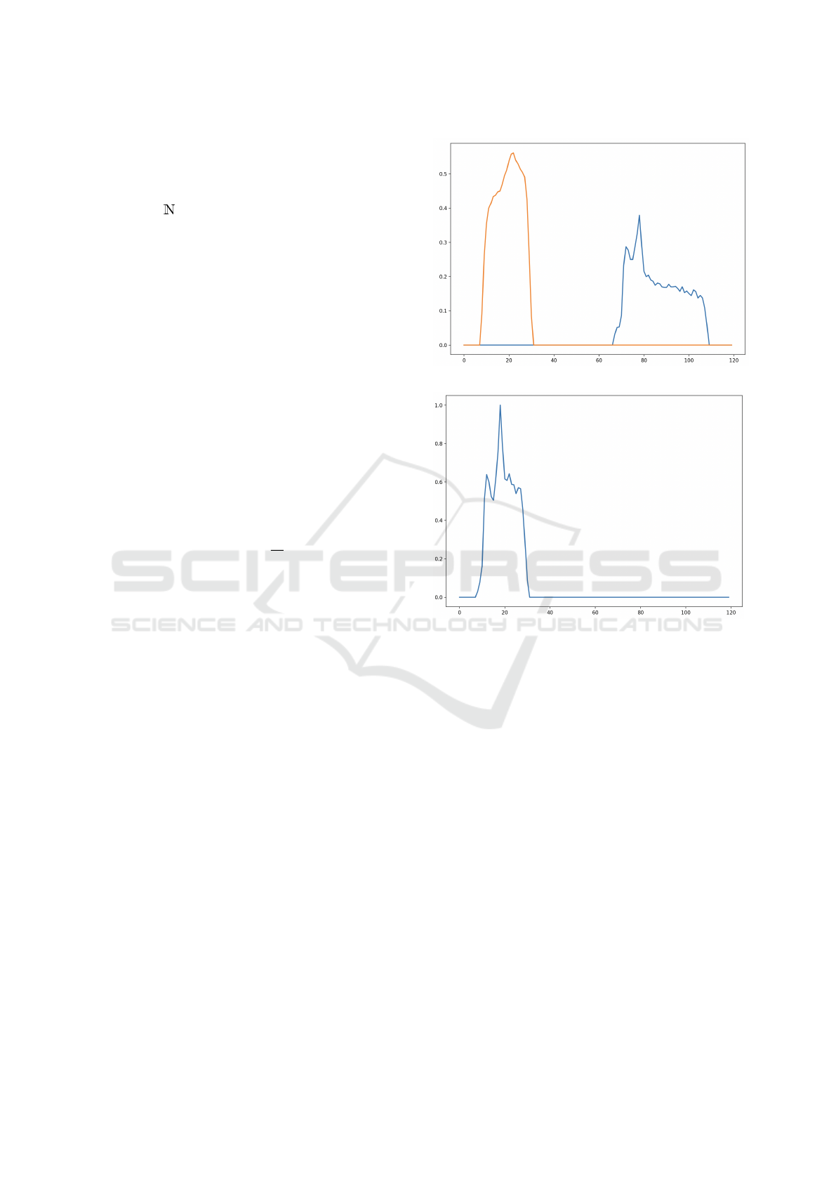
(a) RLM histogram
(b) Force histogram
Figure 3: Computed descriptors for the spatial configura-
tion presented in Fig. 2. The three histograms use Θ = 3
◦
.
(a) Radial Line Model from each object, using the middle
point between the two objects of the image. Object A corre-
sponds to the referent, object B, to the argument. (b) Force
histogram using f
0
around a reference point after Max nor-
malization.
• f
r=0
relies on constant forces which are indepen-
dent of the distance between objects. In some ex-
tent this approach is based on the handling of an
isotropic histogram of angles;
• f
r=2
relies on gravitational forces where more im-
portance is given to closer points.
Fig. 3 provides some examples of RLM and force
histograms for the spatial configuration from Fig. 2.
3.3 Recognition of Spatial Relations
Based on the achieved global spatial relation signa-
tures (extended RLM + forces) between pairs of ob-
jects, we propose a generic framework to translate our
descriptor into spatial relations expressed in natural
VISAPP 2023 - 18th International Conference on Computer Vision Theory and Applications
190

language, and / or potentially into more compact spa-
tial features which can be used in a larger recognition
tasks, for example when a scene is composed of mul-
tiple pairs of objects.
Two main options are possible to translate rela-
tive position descriptors into spatial relations in nat-
ural language: relying on machine learning to auto-
matically generate the transformations, as in (Wang
and Keller, 1999) for the histogram of angles, or using
predefined evaluation rules from theoretical analysis,
as in (Matsakis et al., 2001) for the force histogram.
We propose to use machine learning for our descrip-
tor, by learning the transformation from a dataset an-
notated with object pairs and their spatial relations.
4 EXPERIMENTAL STUDY
We develop three ways to showcase the interest of our
method: the first way aims to show the ability of our
descriptors to capture enough spatial information to
predict spatial relations between object pairs by train-
ing a model on a given dataset. The second one aims
to learn a spatial model from synthetic images and
predict spatial relations in satellite images, while the
third way deals with the denoising of a given ambigu-
ous dataset.
4.1 Datasets
Different datasets of (synthetic or natural) images
were considered in this study. Each image depicts a
scene containing a specific spatial configuration be-
tween a pair of crisp objects, including correspond-
ing annotations. SimpleShapes dataset contains 2280
synthetic images, divided in two distinct sub-datasets
named SimpleShape1 (S1) and SimpleShape2 (S2).
S1 comprises masks of complex objects such as boats
and cars (see Fig. 2), while S2 is composed of convex
and concave geometric objects such as triangles, and
ellipses. Images have been synthesised in a random
way, with no background, and created by generating
random orientation, scale and place on the image. The
GIS dataset is composed of 211 images representing
spatial configurations of geographical objects (e.g.,
houses, river) sensed from aerial images.
Each image of these three datasets contains anno-
tations in which their spatial relations has been as-
sessed by three different experts using the four main
directions (North, West, South, East) (Del
´
earde et al.,
2022). Images were also ranked from N1 to N4 ac-
cording to the difficulty to determine the spatial rela-
tions between the two objects (N1 corresponds to eas-
iest, N4 to ambiguous and/or undecidable). For this
Table 1: Comparison of different methods to compute non-
overlapping reference points (R
p
) in the 2280 images of
the SimpleShapes dataset. Overlapped R
p
does not prevent
computation of RLM and forces but decreases the quality
of the obtained descriptors.
R
p
computation % of R
p
overlapping w/ objects
Straight MBR 71.1%
Oriented MBR 73.7%
Mean of centroids 74.4%
Convex hulls 95.8%
experimental study, N4 images were rejected from the
datasets, lowering the total images used of Simple-
Shapes to 1993, and to 190 images for GIS.
For some experiments, we also considered a sub-
set of the SpatialSense dataset (Yang et al., 2019),
composed of 11570 natural images representing ev-
eryday life scenes (S3), see e.g. Fig. 4. For each
image, SpatialSense provides different spatial annota-
tions (bounding boxes of objects and spatial configu-
rations between them), with spatial relations between
object pairs. We restrict the dataset to images pre-
senting to the left of, above, to the right of, or below
spatial relations, thus reducing the size to 2290 im-
ages. However, some spatial relations are given in a
3-dimensional space. The orientation of subjects and
objects are taken into account when given a spatial
relation, which means the spatial relation may vary a
lot depending on the point of view (2D or 3D). Ac-
cording to our experiences, we may need segmented
objects. We have then pre-processed this dataset to
obtain regions corresponding to the objects of interest
via a segmentation performed in the bounding boxes
provided in the annotations (Del
´
earde et al., 2021).
4.2 Directional Relation Classification
We aim in this preliminary experiment to showcase
the ability of the proposed method to predict direc-
tional spatial relations from the images characterized
by our descriptors, and the importance of using con-
vex hulls as the basis to obtain the reference point R
p
.
4.2.1 Experimental Protocol
As mentioned in Sec. 2 different methods can be em-
ployed to determine the reference point R
p
, such as
straight MBR, oriented MBR and mean distance to
barycenters of both objects. In cases where R
p
over-
laps with an existing object, results from the RLM
may vary a lot and can create errors in classification.
We aim to minimize the average number of images
where the reference point R
p
overlaps with an ob-
ject while still retaining a correct position to obtain
the necessary information to predict the spatial rela-
tion of the two objects. A comparative study of the
An Extension of the Radial Line Model to Predict Spatial Relations
191

Figure 4: A SpatialSense image containing an ambiguous
annotation. The image connects the bicycle in the fore-
ground, to the woman on the left, considers in the anno-
tations ”Bicycle to the left of woman”, but the bicycle is on
the right of the woman.
behavior of the different methods possible to com-
pute R
p
is provided in Tab. 1, using the SimpleShapes
dataset. This preliminary result confirms our intuition
and highlights the interest of using convex hulls as the
basis to obtain the reference point. We will then only
consider this approach to compute our descriptors.
We now illustrate the ability of the proposed
method to predict directional spatial relations. For
this experiment, we use the whole S1 and S2 datasets
individually. In order to showcase the ability of our
method to predict correct spatial relations from these
object configurations, we compute for each pair the
extended RLM of each object and the forces associ-
ated with the relation (RLM + f
2
). For RLM and force
histograms, we considered 120 values (Θ = 3
◦
) lead-
ing to a final feature vector of dimension 360.
Given these image representations, we trained dif-
ferent models to predict the correct spatial relation:
Support-Vector Machine (SVM), k-Nearest Neigh-
bors (k-NN), and Random Forests (RF). The three
models were implemented with default parameters.
As a comparison method, we implemented another
strategy relying only on the bounding boxes of the
object pairs (B-Box approach), which is similar to
the method “2D-only” of SpatialSense (Yang et al.,
2019). Technically, an image containing a spatial con-
figuration can be characterized by considering the co-
ordinates of all bounding boxes of objects. For this
approach, the same classifiers have been considered.
For each tested approach, we used a 5-fold cross-
validation (to learn on 80% of the data), and computed
accuracy and standard deviation of cross-validation
on test sets (20% of the data).
4.2.2 Results
The obtained results are presented in Tab. 2. Over-
all, the models trained from our descriptors or the
comparative B-Box approach offer very good perfor-
mance (with an accuracy greater than 0.9 and a low
standard deviation). However, using the extended
Table 2: Classification of directional relations. Compari-
son of accuracy and standard deviation of cross-validation
on test sets using different supervised models fed with ra-
dial line models and forces (RLM + f
2
) and models with
bounding box coordinates (B-Box).
SVM k-NN RF
S1 (B-Box) 0.95±0.02 0.90±0.02 0.91±0.02
S2 (B-Box) 0.96±0.01 0.93±0.02 0.94±0.01
S1 (RLM) 0.93±0.03 0.91±0.03 0.92±0.03
S2 (RLM) 0.95±0.02 0.94±0.03 0.94±0.02
S1 (RLM + f
2
) 0.93±0.02 0.93±0.03 0.95±0.01
S2 (RLM + f
2
) 0.97±0.01 0.96±0.01 0.97±0.01
RLM with forces allowed to average +0.02 in accu-
racy with almost no changes in the standard deviation
of the cross-validation method. The only model per-
forming worse compared to the bounding box coordi-
nates is the SVM on the S1 dataset.
This first study shows the discriminability capac-
ity of directional spatial configurations between ob-
jects offered by our descriptors as well as its compa-
rability to a (naive but) state-of-the-art approach.
4.3 Synthetic to Natural Configurations
In a second experiment, we present a practical use
case of our spatial relationship prediction method.
Despite the lack of annotated data (with this type of
spatial information) in the literature, we want here to
show that it is possible to learn powerful spatial mod-
els from synthetic data and to transfer these models to
deal with natural images containing realistic spatial
configurations.
4.3.1 Experimental Protocol
This experiment uses the same (synthetic) datasets as
the former experiment with the addition of the GIS
dataset composed of natural images. This experiment
aims to show the ability of the extended Radial Line
Model to predict spatial relations of natural images
from a learning on another dataset.
As discussed in Sec. 3.2, for each object pair,
we compute the spatial relation signature R(X,R
p
),
composed of the both radial line models of each ob-
ject, and the force histogram between the referent and
the argument. We use a value of Θ=3°, which means
each histogram comprises 120 values, leading to a fi-
nal feature vector of dimension 360. The tested ap-
proach uses a Multi-Layer Perceptron (MLP) of 4 hid-
den layers of 448 units each with a ReLU activation
function, and Adam Optimizer (with initial learning
rate of 10
−3
, β
1
= 0.9, β
2
= 0.999, and ε = 10
−8
).
For comparative purposes, different other models
have been implemented and evaluated:
VISAPP 2023 - 18th International Conference on Computer Vision Theory and Applications
192

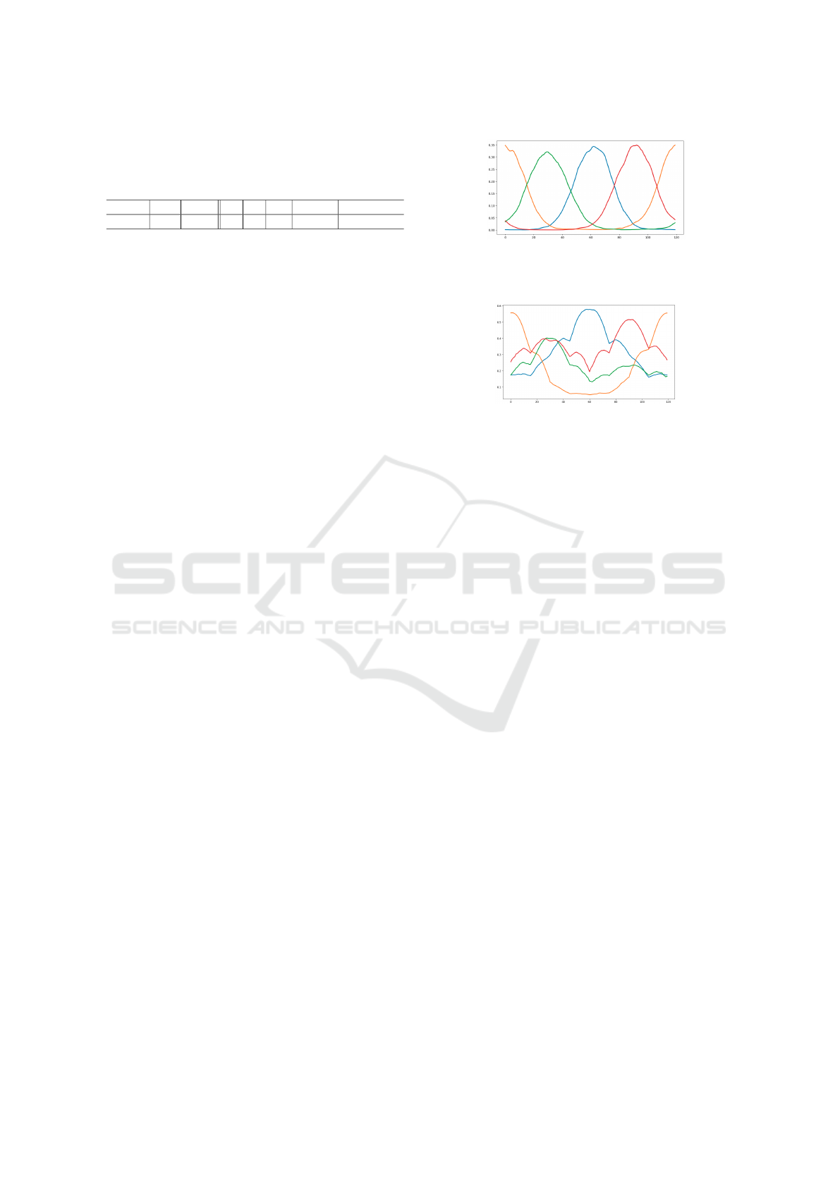
Table 3: Transfer: From synthetic configurations to natural
ones. Comparison of different models trained on SS syn-
thetic datasets and then used to predict spatial relations from
the GIS dataset.
Model B-Box RLM
init
f
0
f
2
RLM RLM + f
2
RLM + f
0
+ f
2
Accuracy 75% 83% 72% 79% 87% 90% 93%
• as baseline, the B-Box approach and the initial
RLM model (Santosh et al., 2012);
• a model using a 240-dimensional vector built
from the spatial relation signature R(X,R
p
)
(without force information);
• models using only a 120-dimensional vector, the
force histogram ( f
0
, f
2
).
This choice aims to demonstrate the relevance of
combining different information to obtain a model
more robust than each descriptor considered individ-
ually. The parameters of the MLP remain the same.
We train each model on the two synthetic datasets
(S1+S2) and employ a cross-validation strategy, with
five subsets (of 20% of the samples each) as test sets.
4.3.2 Results
Each model trained is then applied to predict spatial
relations on the 190 GIS segmented images. Most of
the image contain easily found relationships (118 im-
ages with N1 level) and contain mostly horizontal re-
lationships, with 86 to the left of and 49 to the right
of (see (Del
´
earde et al., 2022)). Tab. 3 presents the
percentage of correctly found relations for each tested
model. Using only forces, first with f
0
and then with
f
2
, the accuracy of the models reach between 72% and
79%, while using only RLM of each object reaches
an accuracy of 87%. f
2
providing better overall re-
sults, we used this type of forces to combine with the
RLM. The accuracy of the prediction shows slightly
better although considerable improvements. By com-
bining the Radial Line Model of both objects, with
both types of forces used before, we obtain a more
robust and better model with better accuracy.
4.4 Dataset Denoising
In this last experiment, we show how our method can
be practically implemented to correct datasets con-
taining (human) spatial annotations that may be er-
roneous or ambiguous.
4.4.1 Experimental Protocol
The last experiment aims to provide a correction of
the SpatialSense (S3) dataset. As mentioned ear-
lier, this dataset contains annotations about the spa-
tial relations between objects present in the images.
Figure 5: Prototypes of each spatial relation class in the
SimpleShapes dataset (to the right of in orange, above in
green, to the left of in blue, under in red).
Figure 6: The prototypes of the to the left of and to the
right of each mix two curves, the bigger one corresponds
to the 2D viewpoint, while the smaller one regroups all of
the wrongly annotated spatial relations (3D viewpoint). The
prototypes of the above and under although not as affected,
still display forms of noise created by 3D viewpoints.
However, as it has been annotated by humans, via
crowd-sourcing campaigns, some annotations can be
ambiguous because they depend on human interpre-
tation. In particular, directional spatial relations are
very sensitive to the viewpoints (2D/3D) and the rep-
resentation of the scene (e.g. Fig. 4). This can lead to
inconsistent learning and erroneous predictions.
To further illustrate this problem of ambiguity, we
propose in a preliminary experiment to build and visu-
alize, for each class of spatial relationship of a dataset,
the prototypes obtained by averaging, for all the im-
ages belonging to a class, the proposed spatial relation
descriptors. It is interesting to compare the prototypes
obtained from the clean SimpleShapes dataset (Fig. 5)
to the ones obtained on the noisy SpatialSense dataset
(Fig. 6) to further motivate the need of denoising it.
The goal of this experiment is then to provide au-
tomatic corrections of these spatial relations. As pre-
viously, we focus here solely on the four main direc-
tional spatial relations. Out of all available images in
the test set of S3, 100 labels have been manually cor-
rected to match spatial relations in a 2-dimensional
space. Most of the corrections are done on the left-
right axis, as most of the ambiguity in the dataset are
based on the orientation of objects in the space. Few
objects in the images had an orientation which lead
to a different interpretation depending on the number
of dimension chosen. This manual correction leads to
a cleaned test set of S3 that we will consider later as
a ground truth to evaluate the impact of our dataset
denoising strategy.
An Extension of the Radial Line Model to Predict Spatial Relations
193

Table 4: Cleaning process of the training set of SpatialSense
(S3). For each class of the initial (noisy) dataset, the table
illustrates the distribution of the new spatial labels assigned
to the configurations.
Cleaned labels
Initial label # images Under Right Above Left
Under 597 197 194 104 102
Right 498 52 236 58 152
Above 429 68 60 191 110
Left 666 70 241 84 271
Table 5: Classification results of each model on the 100
hand-made corrections of S3. The models were trained ei-
ther on the noisy version of S3, or on its clean version.
Training Model Accuracy
Noisy S3 B-Box 0.36
RLM + forces (bboxes) 0.46
RLM + forces (segment.) 0.29
Cleaned S3 B-Box 0.83
RLM + forces (bboxes) 0.93
RLM + forces (segment.) 0.95
To denoise a dataset like SpatialSense, we propose
to learn a clean model for predicting spatial relation-
ships from a synthetic dataset like SimpleShapes. We
propose to use as models the prototypes stated above
(Fig. 5) computed by aggregating the spatial signa-
tures for each class on S1+S2. From this model, the
next step is to apply it to the S3 training set to correct
one by one the annotations of the images that may
contain errors. This can be done by a calculation of
affinity scores between the representation of the im-
age tested and the set of prototypes of the model. De-
pending on the obtained result, the spatial label of
the image is corrected or not. This process leads to
a cleaned S3 dataset, which can then be considered
to train a model of spatial relationship predictions,
which can be tested on the ground truth set.
To showcase the added value of this process, we
can compare the performance on the ground truth of
a model trained on the cleaned version of the dataset
versus a model trained on the initial noisy version of
the dataset. Here different representations were com-
pared, with the objective to highlight the interest of
the force information and the radial line models: (1) A
strategy relying only on the coordinates of the bound-
ing boxes of the object pairs (B-Box approach). A
scene is then described by 8 integers: 4 for each object
(x
min
,x
max
,y
min
, and y
max
); (2) A strategy that consid-
ers the bounding box of each object (initially provided
in the annotations of S3) as crisp regions on which to
apply combination of the forces and the RLM (same
parameters as in Sec. 4.2). Note that simplifying the
object as a bounding box leads in some cases to boxes
overlapping each other and creating wrong relations.
In some other cases, the bounding boxes created for
objects did not fit correctly the objects whose topol-
ogy had a center of gravity far away from the center
of the corresponding bounding box; (3) A strategy to
correct the problems listed above which was imple-
mented using relatively precise object segmentations
of the S3 images thanks to (Del
´
earde et al., 2021).
It allows for more precise topology of objects to be
used. The forces and the RLM are then computed
from these regions. As in Sec. 4.3, we use a MLP
to learn a model from these representations to predict
the relations.
4.4.2 Results
As preliminary results, Tab. 4 presents the outputs
of the cleaning process applied to the training set of
S3 thanks to the prototypes learnt on S1+S2. As ex-
pected, most of the relationships that were corrected
were horizontal (left, right) and were ambiguous due
to the point of view considered.
To evaluate the impact of the denoising step and
the interest of learning on a clean dataset, Tab. 5 pro-
vides the classification results (accuracy) of each as-
sessed model on the 100 hand-made corrections of S3
which is considered as ground-truth. As observation,
the combination of RLM and force information car-
ries more useful spatial information to discriminate
the different spatial configurations than the B-Box
model. Furthermore, on a natural image dataset such
as SpatialSense, we also note the interest of consider-
ing regions that realistically approximate the objects
of interest whose spatial configurations are studied.
5 CONCLUSION
To model spatial relations between object pairs, the
proposed approach combines the Radial Line Model
and the forces histogram computed from a reference
point, computed from the convex hulls of objects.
Used as an image representation, this model outper-
forms state-of-the-art models in classifying spatial
configurations of objects, albeit in a negligible slower
time. The extended RLM can transfer spatial relations
from one dataset to another one, and also denoise
datasets subjected to the human error of viewpoint
on images. This novel approach could further be im-
proved by employing a convolutional neural network
architecture to learn the representation in an end-to-
end fashion. Another improvement could be made by
using a morphological operator such as the geodesic
distance to extract the reference point, to better take
into account concave objects.
VISAPP 2023 - 18th International Conference on Computer Vision Theory and Applications
194

REFERENCES
Bloch, I. (1999). Fuzzy Relative Position between Objects
in Image Processing: A Morphological Approach.
IEEE TPAMI, 21(7):657–664.
Cl
´
ement, M., Poulenard, A., Kurtz, C., and Wendling, L.
(2017). Directional Enlacement Histograms for the
Description of Complex Spatial Configurations be-
tween Objects. IEEE TPAMI, 39(12):2366–2380.
Cohn, A., Bennett, B., Gooday, J., and Gotts, N. (1997).
Qualitative spatial representation and reasoning with
the region connection calculus. GeoInformatica,
3(1):275–316.
Del
´
earde, R., Kurtz, C., Dejean, P., and Wendling, L.
(2021). Segment my object: A pipeline to extract seg-
mented objects in images based on labels or bounding
boxes. In VISAPP, pages 618–625.
Del
´
earde, R., Kurtz, C., and Wendling, L. (2022). Descrip-
tion and recognition of complex spatial configurations
of object pairs with force banner 2d features. PR,
123:108410.
Egenhofer, M. and Franzosa, R. (1991). Point-set topologi-
cal spatial relations. Int. J. GIS, 2(5):161–174.
Freeman, J. (1975). The Modelling of Spatial Relations.
CGIP, 4(2):156–171.
Matsakis, P., Keller, J. M., Wendling, L., Marjamaa, J., and
Sjahputera, O. (2001). Linguistic description of rela-
tive positions in images. IEEE TSMC, 31(4):573–88.
Matsakis, P. and Naeem, M. (2016). Fuzzy Models of Topo-
logical Relationships Based on the PHI-Descriptor. In
FUZZ-IEEE, pages 1096–1104.
Matsakis, P. and Wendling, L. (1999). A new way to repre-
sent the relative position between areal objects. IEEE
TPAMI, 21(7):634–643.
Peyre, J., Laptev, I., Schmid, C., and Sivic, J. (2019).
Weakly-Supervised Learning of Visual Relations. In
ICCV, pages 5189–5198.
Rosenfeld, A. and Klette, R. (1985). Degree of adjacency
or surroundedness. PR, 18(2):169–177.
Santosh, K. C., Lamiroy, B., and Wendling, L. (2012). Sym-
bol recognition using spatial relations. Pattern Recog-
nit. Lett., 33(3):331–341.
Santosh, K. C., Wendling, L., and Lamiroy, B. (2014). Bor:
Bag-of-relations for symbol retrieval. Int. J. Pattern
Recognit. Artif. Intell., 28(6).
Vanegas, M. C., Bloch, I., and Inglada, J. (2011). A fuzzy
definition of the spatial relation “surround” - Applica-
tion to complex shapes. In EUSFLAT, pages 844–851.
Wang, X. and Keller, J. M. (1999). Human-based spatial
relationship generalization through neural/fuzzy ap-
proaches. Fuzzy Sets Syst., 101(1):5–20.
Yang, K., Russakovsky, O., and Deng, J. (2019). Spa-
tialsense: An adversarially crowdsourced benchmark
for spatial relation recognition. In ICCV, pages 2051–
2060.
An Extension of the Radial Line Model to Predict Spatial Relations
195