Fine-Tuning Restricted Boltzmann Machines Using No-Boundary

Jellyﬁsh

Douglas Rodrigues

, Gustavo Henrique de Rosa

, Kelton Augusto Pontara da Costa

Danilo Samuel Jodas

and Jo

ao Paulo Papa

Department of Computing, S

ao Paulo State University, Bauru, Brazil

Keywords:

Computing Methodologies, Reconstruction, Neural Networks, Bio-Inspired Approaches.

Abstract:

Metaheuristic algorithms present elegant solutions to many problems regardless of their domain. The Jellyﬁsh

Search (JS) algorithm is inspired by how jellyﬁsh searches for food in ocean currents and performs movements

within the swarm. In this work, we propose a new version of the JS algorithm called No-Boundary Jellyﬁsh

Search (NBJS) to improve the convergence rate. The NBJS was applied to ﬁne-tune a Restricted Boltzmann

Machine (RBM) in the context of image reconstruction. For validating the proposal, the experiments were

carried out on three public datasets to compare the performance of the NBJS algorithm with its original version

and two other metaheuristic algorithms. The results showed that proposed approach is viable, for it obtained

similar or even lower errors compared to models trained without ﬁne-tuning.

1 INTRODUCTION

Metaheuristic algorithms have gained considerable

popularity in solving combinatorial problems that un-

til now were considered impractical due to high com-

putational costs. Problems like the traveling sales-

man (Wang et al., 2003; Hatamlou, 2018) and the

backpack problem (Hembecker et al., 2007) are just

a few examples where we employ metaheuristic algo-

rithms to ﬁnd feasible solutions.

In machine learning, metaheuristic algorithms

have also played a notable role in improving the

model’s performance, especially in neural network

optimization. Kuremoto et al. (Kuremoto et al.,

2012) employed the Particle Swarm Optimization to

ﬁnd the correct number of units and hyper-parameter

ﬁne-tuning to the context of time series forecasting.

Moreover, Papa et al. (Papa et al., 2015) applied the

Harmony Search in the context of Bernoulli RBM’s

hyper-parameters ﬁne-tuning. In the same context,

Papa et al. (Papa et al., 2016) applied the Harmony

Search to ﬁne-tune Deep Belief Networks (DBN)

hyper-parameters. Later, Passos et al. (Passos et al.,

https://orcid.org/0000-0003-0594-3764

https://orcid.org/0000-0002-6442-8343

https://orcid.org/0000-0001-5458-3908

https://orcid.org/0000-0002-0370-1211

https://orcid.org/0000-0002-6494-7514

2019) compared six meta-heuristic algorithms to ﬁne-

tune the hyper-parameters of an inﬁnity RBM to the

context of automatic identiﬁcation of Barrett’s esoph-

agus from endoscopic images of the lower esophagus.

The success achieved by metaheuristic algorithms

is because they are independent of the problem do-

main and can ﬁnd near-optimal solutions in a rea-

sonable time. In addition, such algorithms can solve

non-linear, non-differentiable, and complex numeri-

cal optimization problems. However, the balance be-

tween exploration and exploitation behaviors is cru-

cial for such algorithms to perform well and avoid get-

ting stuck in local optima. Exploration is the search

for potential solutions in unexplored areas, while ex-

ploitation is the search for better neighboring solu-

tions in promising regions. In this fashion, Chou

and Truong (Chou and Truong, 2021) developed the

novel Jellyﬁsh Search (JS) algorithm inspired by the

behavior of jellyﬁsh’s motion inside the swarm and

the search for food in ocean currents. The algorithm

adopts a time control mechanism to balance the explo-

ration where the jellyﬁsh follow the ocean currents in

search of food and the exploitation behavior in which

the jellyﬁsh moves within the swarm.

In this context, the present work proposes a new

version of the JS algorithm called No-Boundary Jelly-

ﬁsh Search (NBJS) for ﬁne-tuning RBM parameters.

Therefore, the main contributions of this work are:

Rodrigues, D., Henrique de Rosa, G., Pontara da Costa, K., Jodas, D. and Papa, J.

Fine-Tuning Restricted Boltzmann Machines Using No-Boundary Jellyﬁsh.

DOI: 10.5220/0011643400003417

In Proceedings of the 18th International Joint Conference on Computer Vision, Imaging and Computer Graphics Theory and Applications (VISIGRAPP 2023) - Volume 4: VISAPP, pages

65-73

ISBN: 978-989-758-634-7; ISSN: 2184-4321

 2023 by SCITEPRESS – Science and Technology Publications, Lda. Under CC license (CC BY-NC-ND 4.0)

• to introduce the NBJS and JS algorithm in the

context of optimizing RBM’s parameters for the

image reconstruction task; and

• to provide an in-depth comparative analysis be-

tween the JS algorithm and the Black Hole Al-

gorithm (BH) (Hatamlou, 2018) and Particle

Swarm Optimization (PSO) (Kennedy and Eber-

hart, 2001) algorithms in terms of effectiveness

and efﬁciency.

The remainder of this paper is organized as fol-

lows: Section 2 presents some theoretical background

concerning Restricted Boltzmann Machines, JS and

NBJS algorithms, respectively, while Section 3 dis-

cusses the methodology employed in this work. Sec-

tion 4 presents the experimental results and Section 5

states conclusions and future works.

2 THEORETICAL FOUNDATION

In this section, we present a theoretical foundation

concerning Restricted Boltzmann Machines and Jel-

lyﬁsh Search.

2.1 Restricted Boltzmann Machines

Restricted Boltzmann Machines (Ackley et al., 1988;

Hinton, 2012) are generative stochastic neural net-

works belonging to a class of energy-based models.

In such models, we have an energy value associated

with each state of the system. Basically, RBMs con-

sist of m neurons in the visible layer v = (v

, . . . , v

)

and n neurons in the hidden layer h = (h

, . . . , h

Thus, the probability of the system being in a certain

state is given by the Gibbs distribution:

p(v, h) =

−E(v,h)

, (1)

where Z =

∑

v,h

−E(v,h)

is a partition function. The

energy function is described as follows:

E(v, h) = −

∑

i=1

−

∑

j=1

−

∑

i=1

∑

j=1

i j

, (2)

where W is the weight associated with the connection

of the neurons of the visible layer and the invisible

layer, and a and b represent the biases of visible and

hidden units, respectively.

In RBMs, connections between layers are bidirec-

tional, but connections between neurons belonging to

the same layer are not allowed. In this way, the states

of the visible and invisible layers are conditionally in-

dependent and can be described as follows:

p(v) =

∏

p(v

|h) and p(h) =

∏

p(h

|v). (3)

Essentially, training RBMs consists of minimizing

the expected log-likelihood for a training sample v,

given by:

argmin

E[−log p(v)]. (4)

We can compute the gradient of − log p(v) easily

as follows:

∂ − log p(v)

∂W

= E

∂E(v, h)

∂W

− E

v,h

∂E(v, h)

∂W

, (5)

where the ﬁrst term is responsible for increasing the

probability of the data and can be obtained through

conditional probabilities, and the second term is re-

sponsible for reducing the probability of samples gen-

erated by the model. Since this term corresponds to

an intractable problem, we can approximate it using

contrastive divergence training (Hinton, 2002).

2.2 Jellyﬁsh Search

Jellyﬁsh Search was proposed by Chou and

Troung (Chou and Truong, 2021) inspired by how

jellyﬁshes live in waters of different temperatures

and depths. Let X = {x

, x

, . . . , x

} a population

of jellyﬁshes, such that x

∈ R

, ∀i = {1, 2, . . . , m}

represents the position of the i−th jellyﬁsh in a

n−dimensional search space. The Jellyﬁsh Search

is built on three fundamental rules: (i) a mechanism

called “time control” that controls the movement by

deciding whether the jellyﬁsh will follow the ocean

current or will follow the swarm; (ii) jellyﬁshes are

preferentially attracted to places where the concen-

tration of food is higher; and (iii) the amount of food

available at a given location is deﬁned by the location

and its corresponding objective function.

In the ocean current, there is a large amount of

food, making the jellyﬁsh concentrate on it. The di-

rection of the ocean current is given as follows:

−−−→

trend = x

best

− β ∗ ε ∗ µ

µ, (6)

where x

best

is the jellyﬁsh with the best location, β > 0

is the distribution coefﬁcient that controls the length

of the

−−−→

trend, ε ∈ U(0, 1), and µ

µ ∈ R

is the mean lo-

cation of all jellyﬁshes.

Thus, the new location of each jellyﬁsh is given

by:

t+1

= x

+ ϕ ∗

−−−→

trend, (7)

where ϕ ∈ U(0, 1).

VISAPP 2023 - 18th International Conference on Computer Vision Theory and Applications

As the ocean current temperature changes, jelly-

ﬁshes switch ocean currents and form new swarms.

Over time, a swarm is formed with the jellyﬁsh com-

ing together. The movements of a jellyﬁsh within the

swarm can be (i) passive motions (type A) and (ii) ac-

tive motions (type B). The passive motion is described

as follows:

t+1

= x

+ η ∗ φ ∗ (U

− L

), (8)

where η > 0 is the motion coefﬁcient, φ ∈ U(0, 1),

and U

∈ R

and L

∈ R

are the upper and lower

bound, respectively.

The active motion can be described as follows:

t+1

= x

+ (ψ ∗

−−→

step), (9)

where ψ ∈ U(0, 1) and step is deﬁned by:

−−→

step =

(

− x

, if f (x

) ≥ f (x

)

− x

, otherwise

where f (.) denotes the ﬁtness function.

The time control mechanism regulates jellyﬁsh’s

movement and makes them change their behavior be-

tween following the ocean current or moving within

the swarm. The mechanism comprises a time con-

trol function c(t) and a constant C

. The time control

function c(t) can be obtained as follows:

c(t) =





1 −



∗ (2 ∗ λ − 1)



, (10)

where t is the current iteration, T is the total num-

ber of iterations, and λ ∈ U(0, 1). If c is greater

than C

, jellyﬁshes follow the ocean current; other-

wise, they move within the swarm. Also, the time

control mechanism is used to control the movement

performed by jellyﬁsh within the swarm being Type

A if U(0, 1) ≥ (1 − c(t)) or Type B otherwise.

2.3 No-Boundary Jellyﬁsh Search

In Type A movement, the jellyﬁsh moves around its

location. The purpose of this work is to improve the

convergence rate by changing Equation 8, which is

responsible for the exploitation, as follows:

t+1

= X

+ η ∗ φ, (11)

where η > 0 is the motion coefﬁcient, and φ ∈

U(0, 1). By removing the multiplicative factor (U

−

) from Equation 8, the magnitude of the motion

is reduced, making the jellyﬁsh explores the region

around it with higher quality.

3 METHODOLOGY

3.1 Experimental Setup

In this work, we proposed enhancing the RBM recon-

structive capacity by ﬁne-tuning the parameters using

the No-Boundary Jellyﬁsh Search algorithm. Brieﬂy

speaking, we trained an RBM model with the follow-

ing hyper-parameter settings: the learning rate η =

0.1, weight decay λ = 0, and momentum ϕ = 0. For

the number of neurons in the hidden layer, we used

three different settings: n = 128, n = 256, and n = 512

represented by the symbols α, β, and γ, respectively.

Concerning the number of epochs, we have employed

T = 1, 10, 25, 50, 100 with mini-batches of size 128.

Also, the image sizes adopted were: 7 × 7, 14 × 14,

28 × 28.

After the model has been trained, the next step is

ﬁne-tuning the parameters. In RBM, more speciﬁ-

cally, if we look at Equation 2, we have the vector

a that represents the bias of the visible layer, and

the vector b that represents the bias of the invisible

layer. Finally, we have the matrix W that represents

the weights of all connections between the visible and

invisible layers. In the optimization task, we used two

different approaches: (i) selecting the best values for

the vector a, or (ii) selecting the best values for the

matrix W

Brieﬂy explaining the process, the agents that

make up the meta-heuristic algorithm are initialized

with random values by the search space. At each it-

eration, the agents are evaluated in the search space.

In other words, for each evaluated agent, the RBM

model, previously trained, has its parameter (a or W)

replaced by the agent’s current position in the search

space. Then, this new model is validated using a vali-

dation set, and the Mean Square Error (MSE) is com-

puted. At the end of the optimization process, the

previously trained model will have its parameter re-

placed by the position of the best agent, i.e., the set of

parameters that minimizes the MSE in the validation

set.

Given the values that makeup a or W of the trained

model, the lower bound (lb) and upper bound (ub) of

the decision variables are given by:

lb = param − ∆ and ub = param + ∆, (12)

It was decided to optimize only the bias a and the

weight matrix W to test the proposal and then extend it to

other network parameters. As it is a new proposal, the be-

haviour of these experiments was not known.

Our source code is available at https://github.com/

gugarosa/rbm tuning.

Fine-Tuning Restricted Boltzmann Machines Using No-Boundary Jellyﬁsh

where param means a or W, and ∆ = 0.1, 1.0. Fig-

ure 1 depicts the aforementioned methodology con-

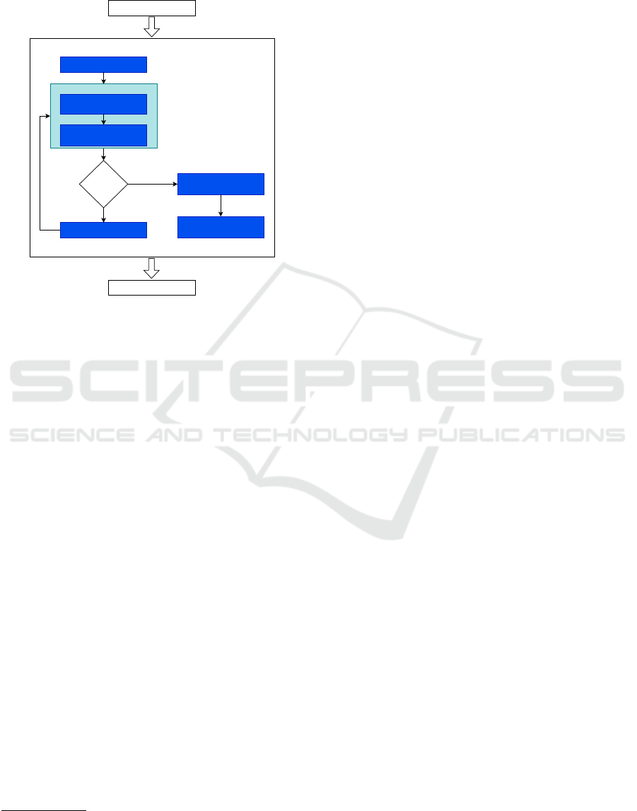
cerning ﬁne-tuning RBM’s parameters.

Initialize population

Replace the params by

the agent's position

Evaluating its validation

accuracy

Update population

Replace the params by

the agent's position

Return the optimized

model

TRAINING

TESTING

Meeting stop

criteria?

Evaluate the population

Yes

OPTIMIZATION

Figure 1: Pipeline of the optimization process.

3.2 Datasets

We employed three datasets, described as follows:

• MNIST dataset: it is composed of images of hand-

written digits. The original version contains a

training set with 60,000 images from digits ‘0’ to

‘9’, as well as a test set with 10,000 images.

• KMNIST dataset: it is composed of articles im-

ages. The dataset contains a training set of 60,000

examples and a test set of 10,000 examples.

• FMNIST dataset: it is composed of 70,000 images

of Japonese handwritten digits.

4 EXPERIMENTAL RESULTS

This section presents the results regarding ﬁne-tuning

RBM’s parameters over MNIST, FMNIST, and KM-

NIST datasets. We carried out the experimental

phase in two stages: (i) convergence analysis; and

(ii) reconstruction analysis. For statistical pursuits

and robust analysis, we used Wilcoxon’s signed-rank

test (Wilcoxon, 1945) adopting p = 0.05 on the re-

sults from 25 independent cross-validation runs. For

comparison purposes, besides No-Boundary Jellyﬁsh

Search and Jellyﬁsh Search algorithms, we also used

the Black Hole and Particle Swarm Optimization al-

gorithms available at Opytimizer library

. Thus, the

https://github.com/gugarosa/opytimizer.

results that compose this work are presented in terms

of mean and standard deviation. Notice that the best

results are highlighted in bold. Finally, we adopted 10

agents over 15 iterations for all techniques.

4.1 Reconstruction Analysis

Table 1 presents the results obtained considering the

models trained in the training set and, later, evaluated

in the test set without any optimization. Such results

will serve as the baseline for comparison purposes

with the method proposed in this work. Tables 2, 3,

and 4 present the results concerning the MNIST, FM-

NIST, and KMNIST datasets, respectively.

To Facilitate and Guide Our Analysis in Under-

standing the Displayed Results, the Superscript

Markers Separate the Groups of Statistically Sim-

ilar Results. Starting with the MNIST dataset, the

ﬁrst group is composed of α and 7 × 7 size images,

where the NBJS and JS showed MSE lower than the

baseline concerning the ﬁne-tune W with ∆ = 1.0

considering 10 epochs of pre-training. In α group,

14 × 14 and 28 × 28 size images, the lowest errors

were achieved by the RBM trained conventionally

without ﬁne-tuning.

Moreover, in β and γ groups, NBJS and JS reached

the lowest MSE to ﬁne-tune W concerning 1 and

10 epochs of pre-training on 7 × 7 size images. In

both cases, the best result was achieved with ∆ = 1.0.

However, regarding the 14×14 size images belonging

to γ group, all the analyzed metaheuristics performed

statistically similar to the models without optimiza-

tion in the ﬁne-tuning of a and W for ∆ = 0.1 and

∆ = 1.0. Furthermore, in the 28 × 28 size images, the

NBJS and JS performed similarly to the unoptimized

models in ﬁne-tuning W with ∆ = 0.1.

Considering the FMNIST dataset, NBJS and JS

achieved the best results in the γ group for the ﬁne-

tuning W with ∆ = 1.0 on the 7 × 7 size images. As

for the α group, in the 7 × 7 and 14 × 14 size im-

ages with ∆ = 0.1 and ∆ = 1.0, respectively, the NBJS

and JS had statistically similar results to the models

without optimization. Finally, for the γ group, in the

14×14 size images, the NBJS and JS had the smallest

errors considering the ﬁne-tuning of W with ∆ = 0.1.

And in the 28 × 28 size images, for the ﬁne-tuning of

a, all algorithms performed statistically similarly for

both ∆ conﬁgurations and ∆ = 0.1 in terms of ﬁne-

tuning the W.

Finally, in the KMNIST dataset, in the 7 × 7 size

images, the PSO obtained the lowest MSE value in

the ﬁne-tuning of the parameter a with ∆ = 1.0 for

the group α. In β and γ groups, the NBJS and the JS

obtained the lowest values of MSE in the ﬁne-tuning

VISAPP 2023 - 18th International Conference on Computer Vision Theory and Applications

Table 1: Non-optimized models’ reconstruction errors over MNIST, FMNIST and KMNIST testing sets.

Models

MNIST FMNIST KMNIST

7 × 7 14 × 14 28×28 7 × 7 14 × 14 28 × 28 7 × 7 14 × 14 28 × 28

RBM-α

6.87 ± 0.03 24.23 ±0.15 87.66 ± 0.39 9.27 ± 0.03 35.11 ± 0.12 144.13 ± 0.71 10.83 ± 0.04 38.69 ± 0.13 160.92 ± 0.84

RBM-α

6.06 ± 0.02 17.39 ±0.05 65.13 ± 0.24 7.64 ± 0.05 26.81 ± 0.09 127.10 ± 0.83 9.70 ± 0.05 31.08 ± 0.11 136.14 ± 0.76

RBM-α

5.81 ± 0.02 16.41 ±0.07 62.71 ± 0.33 7.19 ± 0.04 25.81 ± 0.05

118.78 ± 1.37 9.39 ± 0.04 29.97 ± 0.11 134.41 ± 0.84

RBM-α

5.62 ± 0.05 15.99 ± 0.10

61.06 ± 0.38 7.06 ± 0.04

25.46 ± 0.06

110.92 ± 0.82 9.32 ± 0.03 29.69 ± 0.13

132.94 ± 1.27

RBM-α

100

5.52 ± 0.03 15.79 ± 0.07

59.21 ± 0.47

7.02 ± 0.04

25.24 ± 0.04

106.22 ± 0.62

9.27 ± 0.03 29.62 ± 0.11

130.80 ± 2.08

RBM-β

6.84 ± 0.04 21.65 ±0.07 67.13 ± 0.14 8.58 ± 0.03 30.88 ± 0.12 129.05 ± 0.59 10.47 ± 0.08 35.90 ± 0.12 134.16 ± 0.33

RBM-β

6.05 ± 0.04 15.90 ±0.05 42.30 ± 0.13 7.52 ± 0.01 25.46 ± 0.09 98.29 ± 0.26 9.59 ± 0.05 28.32 ± 0.05 93.06 ± 0.20

RBM-β

5.88 ± 0.02 14.92 ±0.04 37.11 ± 0.16 7.22 ± 0.03 24.81 ± 0.07 92.34 ± 0.21 9.37 ± 0.03 27.14 ± 0.08 85.26 ± 0.15

RBM-β

5.71 ± 0.03 14.39 ±0.05 35.02 ± 0.16 7.06 ± 0.02

24.49 ± 0.06 90.12 ± 0.26 9.29 ± 0.04 26.68 ± 0.06

82.53 ± 0.26

RBM-β

100

5.55 ± 0.04 14.10 ± 0.06

33.75 ± 0.12

7.02 ± 0.04

24.29 ± 0.08

88.85 ± 0.21

9.24 ± 0.02 26.40 ± 0.08

81.00 ± 0.18

RBM-γ

6.80 ± 0.20 20.16 ±0.16 55.37 ± 0.19 8.50 ± 0.07 27.46 ± 0.11 112.07 ± 0.51 10.53 ± 0.23 33.28 ± 0.22 111.28 ± 0.22

RBM-γ

6.06 ± 0.06 15.78 ± 0.05

32.67 ± 0.11

7.53 ± 0.06 25.27 ± 0.08 90.64 ±0.27

9.50 ± 0.08 27.36 ± 0.06 67.79 ± 0.12

RBM-γ

5.91 ± 0.04 14.84 ± 0.05

29.50 ± 0.06

7.26 ± 0.04 24.67 ± 0.07

87.27 ± 0.28

9.45 ± 0.08 26.50 ± 0.04 62.31 ± 0.08

RBM-γ

5.70 ± 0.05 14.35 ± 0.06

28.12 ± 0.04

7.08 ± 0.02 24.36 ± 0.11

85.76 ± 0.31

9.30 ± 0.04 26.06 ± 0.05

60.05 ± 0.10

RBM-γ

100

5.53 ± 0.04 14.03 ± 0.04

27.32 ± 0.04

7.01 ± 0.02 24.14 ± 0.06

84.43 ± 0.25

9.23 ± 0.05 25.81 ± 0.03

58.94 ± 0.07

Table 2: Optimized models’ reconstruction errors over MNIST testing set.

Models

7 ×7 14 × 14 28 × 28

a W a W a W

∆

∆ =

= 0

1 ∆

∆

∆ =

= 1

0 ∆

∆

∆ =

= 0

1 ∆

∆

∆ =

= 1

0 ∆

∆

∆ =

= 0

1 ∆

∆

∆ =

= 1

0 ∆

∆

∆ =

= 0

1 ∆

∆

∆ =

= 1

0 ∆

∆

∆ =

= 0

1 ∆

∆

∆ =

= 1

0 ∆

∆

∆ =

= 0

1 ∆

∆

∆ =

= 1

BH-α

6.84 ±0.03 6.61 ±0.10 6.79 ±0.04 6.40 ± 0.20 24.19 ±0.14 23.98 ± 0.14 24.10 ± 0.17 24.34 ± 0.24 87.64 ±0.40 87.78 ±0.48 87.66 ±0.42 90.87± 0.83

JS-α

6.74 ±0.05 6.59 ±0.40 7.69 ±1.16 5.75 ± 1.19 23.79 ±0.15 24.98 ± 0.89 26.20 ± 1.71 32.59 ± 2.57 86.57 ±0.37 93.56 ±2.95 88.48 ±3.70 127.31 ± 23.45

NBJS-α

6.77 ±0.06 6.76 ±0.37 7.97 ±0.95 6.01 ± 0.74 23.85 ±0.14 24.88 ± 0.75 26.38 ± 2.21 31.34 ± 5.11 86.67 ±0.48 95.05 ±2.20 88.32 ±4.37 121.03 ± 17.06

PSO-α

6.83 ±0.03 6.26 ±0.14 6.69 ±0.05 6.40 ± 0.18 24.19 ±0.15 24.08 ± 0.20 24.05 ± 0.17 25.25 ± 0.50 87.66 ±0.37 88.14 ±0.39 87.77 ±0.42 96.91± 1.72

BH-α

6.04 ±0.02 5.89 ±0.04 5.99 ±0.02 5.76 ± 0.08 17.38 ±0.05 17.35 ± 0.07 17.36 ± 0.05 17.77 ± 0.17 65.14 ±0.25 65.29 ±0.25 65.15 ±0.24 67.14± 0.55

JS-α

6.02 ±0.02 6.04 ±0.22 6.38 ±0.44 5.23 ± 0.28

17.25 ±0.05 18.56± 0.27 17.18 ± 0.41 21.33 ±1.21 64.89 ± 0.28 69.97 ± 1.76 63.20 ± 0.62 78.68 ±5.02

NBJS-α

6.02 ±0.02 6.09 ±0.21 6.46 ±0.32 5.30 ± 0.64

17.27 ±0.07 18.66± 0.46 17.31 ± 0.34 20.44 ±2.13 64.87 ± 0.27 70.84 ± 0.78 62.96 ± 0.34 85.10 ±4.68

PSO-α

6.03 ±0.03 5.70 ±0.11 5.91 ±0.06 5.63 ± 0.19 17.38 ±0.05 17.43 ± 0.10 17.33 ± 0.08 18.56 ± 0.34 65.13 ±0.25 65.52 ±0.29 65.22 ±0.29 70.17± 0.86

BH-β

6.82 ±0.04 6.56 ±0.07 6.68 ±0.06 6.37 ± 0.15 21.63 ±0.06 21.50 ± 0.12 21.52 ± 0.09 22.05 ± 0.48 67.13 ±0.13 67.34 ±0.15 67.17 ±0.13 74.50± 1.02

JS-β

6.88 ±0.06 6.29 ±0.26 13.72 ±1.86 3.23 ±0.26

21.67 ±0.08 20.52± 0.60 26.98 ± 3.96 26.53 ±2.90 66.72 ± 0.11 69.03 ± 1.62 71.59± 13.32 137.08 ± 18.75

NBJS-β

6.86 ±0.07 6.18 ±0.26 10.48 ±3.64 3.32 ±0.33

21.64 ±0.10 20.58± 0.81 21.64 ± 3.38 27.02 ±1.77 66.73 ± 0.18 69.66 ± 2.01 69.96± 13.05 144.85 ± 19.50

PSO-β

6.80 ±0.04 6.22 ±0.12 6.45 ±0.08 6.40 ± 0.40 21.61 ±0.07 21.62 ± 0.11 21.50 ± 0.14 24.51 ± 0.75 67.14 ±0.15 67.61 ±0.18 67.37 ±0.21 86.40± 3.87

BH-β

6.04 ±0.04 5.87 ±0.05 5.92 ±0.04 5.57 ± 0.20 15.89 ±0.05 15.88 ± 0.06 15.84 ± 0.03 16.22 ± 0.17 42.30 ±0.12 42.49 ±0.14 42.40 ±0.12 47.76± 0.84

JS-β

6.07 ±0.04 5.62 ±0.23 7.10 ±1.34 3.22 ± 0.28

15.85 ±0.06 15.96± 0.34 19.18 ± 1.85 21.60 ±2.82 42.31 ± 0.17 43.53 ± 0.51 44.40 ± 4.96 100.76 ± 19.20

NBJS-β

6.07 ±0.06 5.65 ±0.18 7.03 ±1.26 3.20 ± 0.26

15.85 ±0.05 16.24± 0.32 17.09 ± 2.03 20.12 ±3.18 42.31 ± 0.17 43.72 ± 0.47 42.74 ± 3.38 109.93 ± 15.39

PSO-β

6.03 ±0.04 5.74 ±0.08 5.81 ±0.06 5.57 ± 0.41 15.90 ±0.05 15.97 ± 0.06 15.81 ± 0.10 17.33 ± 0.55 42.31 ±0.12 42.70 ±0.09 42.45 ±0.14 56.42± 1.82

BH-γ

6.77 ±0.20 6.56 ±0.22 6.50 ±0.16 6.32 ± 0.31 20.14 ±0.16 20.04 ± 0.14 19.98 ± 0.17 21.76 ± 0.58 55.37 ±0.20 55.50 ±0.20 55.44 ±0.16 64.56± 1.12

JS-γ

6.73 ±0.18 6.15 ±0.29 6.06 ±3.95 1.33 ± 0.06

20.02 ±0.16 18.98± 0.49 14.75 ± 0.52 14.25± 0.74

55.47 ±0.24 55.77 ±0.55 44.36 ±4.02 120.24 ± 11.78

NBJS-γ

6.75 ±0.18 6.08 ±0.19 4.95 ±0.33 1.36 ± 0.07

20.04 ±0.17 19.16± 0.47 14.84 ± 0.58 14.32± 0.64

55.45 ±0.20 56.05 ±0.60 229.20 ±301.12 128.76 ±18.63

PSO-γ

6.75 ±0.20 6.18 ±0.18 6.03 ±0.21 8.14 ± 0.79 20.13 ±0.14 20.09 ± 0.16 19.77 ± 0.22 28.28 ± 1.36 55.38 ±0.19 55.73 ±0.18 55.55 ±0.19 80.94± 5.25

BH-γ

6.04 ±0.06 5.90 ±0.04 5.79 ±0.08 5.52 ± 0.24 15.77± 0.06

15.78 ±0.04

15.58 ±0.07

16.05 ±0.52 32.67 ± 0.11 32.82 ± 0.10 32.78 ± 0.13 40.66 ±1.07

JS-γ

6.01 ±0.06 5.50 ±0.15 5.04 ±0.92 1.36 ± 0.10

15.72 ±0.05

15.65 ±0.23

14.01 ±2.58

15.72 ±1.34

32.63 ±0.10 33.33 ±0.19 32.84 ±9.23

108.16 ±14.30

NBJS-γ

6.01 ±0.06 5.49 ±0.14 4.98 ±0.95 1.34 ± 0.05

15.74 ±0.05

15.71 ±0.24

15.15 ±3.61

15.84 ±0.75

32.63 ±0.10 33.32 ±0.17 30.44 ±2.93

105.50 ±12.80

PSO-γ

6.03 ±0.06 5.64 ±0.12 5.51 ±0.11 6.34 ± 0.37 15.78± 0.06

15.82 ±0.07

15.42 ±0.08

18.14 ±0.70 32.68 ± 0.11 32.93 ± 0.11 32.88 ± 0.12 51.66 ±3.86

of the parameter W with ∆ = 1.0. In 14 × 14 size

images, NBJS and JS obtained similar results in opti-

mizing the parameter W with ∆ = 0.1 and ∆ = 1.0 to

the results obtained without optimization.

The metaheuristic algorithms, especially the

NBJS algorithm, obtained errors similar to or lower

than the models’ errors without ﬁne-tuning. The num-

ber of functions evaluated during an iteration in a

metaheuristic algorithm is equivalent to the number of

agents. Furthermore, the computational cost to eval-

uate the objective function is just replacing the posi-

tions of each agent in the RBM weight matrix. For

Fine-Tuning Restricted Boltzmann Machines Using No-Boundary Jellyﬁsh

Table 3: Optimized models’ reconstruction errors over FMNIST testing set.

Models

7 ×7 14 × 14 28 × 28

a W a W a W

∆

∆ =

= 0

1 ∆

∆

∆ =

= 1

0 ∆

∆

∆ =

= 0

1 ∆

∆

∆ =

= 1

0 ∆

∆

∆ =

= 0

1 ∆

∆

∆ =

= 1

0 ∆

∆

∆ =

= 0

1 ∆

∆

∆ =

= 1

0 ∆

∆

∆ =

= 0

1 ∆

∆

∆ =

= 1

0 ∆

∆

∆ =

= 0

1 ∆

∆

∆ =

= 1

BH-α

9.25 ±0.03 9.16 ±0.04 9.21 ± 0.05 9.12 ± 0.08 35.10± 0.12 34.93 ± 0.15 35.01± 0.10 35.16 ± 0.12 144.12 ±0.70 144.24 ± 0.70 143.98 ±0.68 146.43 ± 0.74

JS-α

9.24 ±0.05 9.17 ±0.13 8.24 ± 0.04 9.65 ± 0.89 34.98± 0.13 35.48 ± 0.41 31.81± 0.18 40.11 ± 2.39 143.87 ±0.69 147.08 ± 1.75 132.62 ±1.77 165.04 ± 13.06

NBJS-α

9.23 ±0.04 9.22 ±0.20 8.21 ± 0.05 10.06 ± 0.83 34.98 ± 0.13 35.46 ± 0.47 31.95 ±0.32 43.06 ± 2.35 143.83 ± 0.69 147.63 ± 1.42 132.79 ± 2.13 170.35 ± 22.75

PSO-α

9.24 ±0.04 9.10 ±0.09 9.15 ± 0.07 9.11 ± 0.22 35.08 ± 0.12 35.07 ± 0.20 34.93 ±0.18 36.62 ± 0.50 144.09 ± 0.68 144.65 ± 0.72 144.11 ± 0.60 151.48 ± 1.79

BH-α

7.63 ±0.04 7.58 ±0.04 7.58 ± 0.05 7.48 ± 0.08 26.80 ± 0.09 26.78 ± 0.09 26.75 ±0.10 27.28 ± 0.29 127.10 ± 0.83 127.19 ± 0.79 126.96 ± 0.82 128.57 ± 1.16

JS-α

7.60 ±0.04 7.67 ±0.07 7.00 ±0.04

8.02 ±0.48 26.75 ±0.10 27.56 ±0.20 25.21 ±0.27

31.74 ±2.49 126.84 ± 0.82 128.96 ±0.80 115.30± 0.74 135.76 ± 4.26

NBJS-α

7.60 ±0.04 7.67 ±0.07 6.99 ±0.03

8.39 ±0.29 26.74 ±0.10 27.52 ±0.19 25.22 ±0.40

33.67 ±3.28 126.87 ± 0.83 128.93 ±1.01 115.35± 0.81 138.35 ± 6.82

PSO-α

7.63 ±0.05 7.60 ±0.05 7.58 ± 0.05 7.72 ± 0.10 26.79 ± 0.09 26.93 ± 0.11 26.74 ±0.11 28.55 ± 0.43 127.06 ± 0.85 127.49 ± 0.90 126.98 ± 0.79 131.47 ± 1.18

BH-β

8.57 ±0.03 8.49 ±0.03 8.50 ± 0.03 8.53 ± 0.23 30.86 ± 0.12 30.79 ± 0.15 30.74 ±0.13 31.73 ± 0.45 129.04 ± 0.57 129.16 ± 0.60 128.92 ± 0.56 134.28 ± 1.34

JS-β

8.54 ±0.03 8.49 ±0.13 8.02 ± 0.51 8.47 ± 0.45 30.84 ± 0.12 31.16 ± 0.28 28.26 ±1.51 42.48 ± 3.28 128.48 ± 0.53 130.94 ± 0.81 111.57 ± 3.72 187.45 ± 26.21

NBJS-β

8.53 ±0.03 8.51 ±0.05 7.89 ± 0.56 8.09 ± 0.46 30.84 ± 0.12 31.09 ± 0.17 27.60 ±0.64 43.96 ± 3.35 128.48 ± 0.52 130.41 ± 0.85 115.17 ± 7.33 194.65 ± 27.40

PSO-β

8.56 ±0.03 8.47 ±0.06 8.44 ± 0.06 8.73 ± 0.28 30.85 ± 0.13 30.92 ± 0.17 30.69 ±0.18 33.59 ± 0.69 129.03 ± 0.61 129.51 ± 0.69 129.05 ± 0.63 144.27 ± 2.77

BH-β

7.51 ±0.01 7.47 ±0.03 7.46 ± 0.04 7.41 ± 0.08 25.45 ± 0.09 25.42 ± 0.11 25.37 ±0.11 26.73 ± 0.32 98.29 ± 0.26 98.44 ± 0.31 98.27 ± 0.32 105.35 ± 0.78

JS-β

7.49 ±0.01 7.57 ±0.06 8.25 ± 1.40 7.61 ± 0.40 25.35 ± 0.09 25.87 ± 0.15 30.44 ±6.31 36.18 ± 2.72 97.70 ± 0.26 98.23 ± 0.47 96.97 ± 7.86 169.09 ± 18.54

NBJS-β

7.49 ±0.01 7.59 ±0.08 8.42 ± 1.12 7.82 ± 0.42 25.34 ± 0.09 25.88 ± 0.22 32.60 ±4.79 37.60 ± 4.40 97.68 ± 0.26 98.28 ± 0.40 97.68 ±10.17 148.84 ± 15.41

PSO-β

7.51 ±0.02 7.50 ±0.04 7.39 ± 0.04 7.57 ± 0.17 25.45 ± 0.09 25.49 ± 0.10 25.36 ±0.08 29.04 ± 0.58 98.29 ± 0.27 98.79 ± 0.32 98.39 ± 0.18 114.54 ± 2.19

BH-γ

8.49 ±0.07 8.39 ±0.05 8.33 ± 0.07 8.58 ± 0.46 27.45 ± 0.11 27.38 ± 0.10 27.39 ±0.11 30.86 ± 0.51 112.05 ± 0.50 112.19 ± 0.44 112.07 ± 0.48 123.33 ± 1.97

JS-γ

8.41 ±0.07 8.27 ±0.13 6.29 ± 0.41 4.93± 0.21

27.21 ±0.11 27.72 ±0.18 33.45± 30.77 35.29 ± 1.60 111.48 ± 0.51 113.08 ± 0.40 134.08 ± 17.21 198.84 ±5.65

NBJS-γ

8.41 ±0.06 8.37 ±0.12 8.76 ± 7.39 7.51 ± 7.83 27.20 ± 0.11 27.77 ± 0.19 42.75 ± 41.22 34.99 ±1.05 111.49 ± 0.51 113.03 ±0.53 93.77 ± 0.98 197.88 ± 10.55

PSO-γ

8.48 ±0.07 8.39 ±0.10 8.12 ± 0.05 9.54 ± 0.57 27.45 ± 0.11 27.51 ± 0.14 27.52 ±0.14 35.83 ± 1.48 112.06 ± 0.50 112.56 ± 0.54 112.32 ± 0.52 138.71 ± 5.22

BH-γ

7.53 ±0.06 7.47 ±0.07 7.38 ± 0.05 7.36 ± 0.26 25.26 ± 0.09 25.25 ± 0.09 25.15 ±0.07 26.79 ± 0.37 90.64 ±0.28

90.82 ±0.27

90.63 ±0.31

106.06 ±1.75

JS-γ

7.48 ±0.06 7.50 ±0.11 6.06 ± 0.31 4.94± 0.18

25.07 ±0.08 25.59 ±0.22 22.42 ± 2.93

33.11 ±3.73 89.84± 0.29

90.04 ±0.82

95.40 ±27.45

172.91 ±21.13

NBJS-γ

7.48 ±0.06 7.56 ±0.09 6.20 ± 0.44 5.14± 0.22

25.06 ±0.08 25.75 ±0.19 22.18 ± 1.21

33.54 ±2.34 89.82± 0.26

90.45 ±0.34

84.27 ±14.87

174.66 ±23.89

PSO-γ

7.52 ±0.06 7.51 ±0.07 7.29 ± 0.09 8.04 ± 0.38 25.26 ± 0.08 25.36 ± 0.14 25.20 ±0.13 29.29 ± 0.88 90.62 ±0.28

91.15 ±0.20

91.01 ±0.39

122.89 ±4.74

Table 4: Optimized models’ reconstruction errors over KMNIST testing set.

Models

7 ×7 14 ×14 28 ×28

a W a W a W

∆

∆ =

= 0

1 ∆

∆

∆ =

= 1

0 ∆

∆

∆ =

= 0

1 ∆

∆

∆ =

= 1

0 ∆

∆

∆ =

= 0

1 ∆

∆

∆ =

= 1

0 ∆

∆

∆ =

= 0

1 ∆

∆

∆ =

= 1

0 ∆

∆

∆ =

= 0

1 ∆

∆

∆ =

= 1

0 ∆

∆

∆ =

= 0

1 ∆

∆

∆ =

= 1

BH-α

10.79 ±0.04 10.39 ± 0.06 10.78± 0.05 10.64 ± 0.14 38.64 ±0.13 38.37 ± 0.16 38.63 ±0.13 38.91 ±0.20 160.84 ± 0.83 160.72 ± 0.89 160.89 ± 0.79 163.86 ± 0.94

JS-α

10.67 ±0.05 9.95 ± 0.97 11.08± 0.62 10.03 ± 0.59 37.73 ±0.14 41.33 ± 1.00 41.01 ±2.18 43.36 ±2.42 157.35 ± 0.80 169.78 ±10.02 163.12 ±6.24 187.36 ±13.69

NBJS-α

10.67 ±0.08 9.67 ± 1.00 11.29± 0.84 9.81 ± 0.30 37.73± 0.12 40.78 ± 1.99 41.12± 1.85 43.93 ± 2.18 157.36± 0.80 167.97 ± 7.81 167.66 ± 6.19 195.96 ± 13.55

PSO-α

10.75 ±0.07 9.83 ± 0.40 10.77± 0.05 10.55 ± 0.32 38.58 ±0.15 38.52 ± 0.41 38.62 ±0.13 40.18 ±0.49 160.81 ± 0.84 161.40 ± 1.04 160.94 ± 0.81 169.29 ± 2.05

BH-α

9.67 ±0.05 9.35 ±0.10 9.66 ±0.04 9.46 ± 0.11 31.06± 0.10 30.91 ± 0.18 31.02± 0.10 31.32 ± 0.15 136.11± 0.78 136.20 ± 0.71 136.10 ±0.80 138.14 ± 0.90

JS-α

9.57 ±0.04 9.93 ±0.41 9.89 ±0.33 9.40 ± 0.43 30.68± 0.09 33.34 ± 0.90 31.23± 0.21 37.01 ± 1.57 134.45± 0.73 141.08 ± 4.49 135.96 ±1.24 163.67 ± 9.29

NBJS-α

9.57 ±0.05 9.74 ±0.65 9.99 ±0.33 9.38 ± 0.35 30.68± 0.09 32.89 ± 1.33 31.27± 0.31 36.51 ± 2.08 134.35± 0.70 140.70 ± 3.12 135.79 ±1.12 157.81 ± 5.66

PSO-α

9.64 ±0.04 8.95 ± 0.22

9.62 ±0.04 9.45 ± 0.17 31.05± 0.10 30.92 ± 0.22 31.03± 0.10 32.58 ± 0.32 136.15± 0.76 136.51 ± 0.80 136.22 ±0.81 141.95 ± 1.28

BH-β

10.44 ±0.08 10.09 ± 0.10 10.30± 0.08 10.28 ± 0.34 35.87 ±0.12 35.51 ± 0.10 35.82 ±0.12 36.29 ±0.31 134.15 ± 0.36 134.22 ± 0.38 134.27 ± 0.37 142.67 ± 1.36

JS-β

10.38 ±0.08 8.71 ± 0.60 7.82 ±1.24 5.97 ± 0.18

35.76 ±0.22 32.49 ± 2.51 36.78 ±2.72 41.26 ±1.86 131.93 ± 0.25 132.90 ± 7.55 130.76 ± 9.51 210.66 ± 7.30

NBJS-β

10.35 ±0.09 9.19 ± 0.62 7.82 ±0.94 5.85 ± 0.31

35.61 ±0.20 33.86 ± 1.74 36.61 ±2.47 41.30 ±1.43 131.85 ± 0.33 138.13 ± 3.98 127.59 ± 7.77 207.93 ±14.93

PSO-β

10.39 ±0.10 9.62 ± 0.25 10.10± 0.15 10.77 ± 0.63 35.84 ±0.15 35.69 ± 0.26 35.82 ±0.14 38.29 ±0.73 134.12 ± 0.36 134.81 ± 0.43 134.46 ± 0.33 156.26 ± 2.89

BH-β

9.56 ±0.06 9.30 ±0.09 9.48 ±0.07 9.18 ± 0.20 28.31± 0.05 28.24 ± 0.11 28.25± 0.06 28.66 ± 0.27 93.07 ± 0.19 93.29 ± 0.26 93.21 ±0.23 100.22 ± 0.53

JS-β

9.47 ±0.08 8.24 ±0.33 10.91± 3.10 6.33 ± 0.30

28.05 ±0.08 27.73 ± 1.24 29.52 ±2.46 35.11 ±3.76 92.31± 0.19 96.76 ±1.75 95.27± 6.74 163.08 ±17.29

NBJS-β

9.47 ±0.06 8.60 ±0.39 12.12± 1.94 6.21 ± 0.28

28.07 ±0.06 28.80 ± 0.84 29.54 ±1.73 35.54 ±2.09 92.36± 0.23 95.20 ±2.44 92.72± 3.55 156.13 ±16.53

PSO-β

9.55 ±0.06 8.86 ±0.28 9.34 ±0.06 9.14 ± 0.46 28.28± 0.04 28.35 ± 0.08 28.26± 0.06 29.75 ± 0.32 93.08 ± 0.20 93.55 ± 0.26 93.37 ±0.23 113.23 ± 3.14

BH-γ

10.49 ±0.22 10.15 ± 0.21 10.22± 0.23 10.61 ± 0.39 33.25 ±0.22 33.00 ± 0.18 33.07 ±0.28 36.83 ±1.18 111.27 ± 0.21 111.54 ± 0.26 111.36 ± 0.22 125.93 ± 2.04

JS-γ

10.29 ±0.21 8.98 ± 0.40 21.64 ± 16.16 2.44 ±0.13

32.60 ±0.20 29.99 ± 1.48 88.35 ±63.59 25.24 ± 0.98

110.24 ±0.19 109.04 ± 2.61 93.20 ± 1.65 170.98 ± 8.96

NBJS-γ

10.26 ±0.20 9.06 ± 0.48 15.91 ± 14.59 2.40 ±0.10

32.59 ±0.21 29.74 ± 1.30 88.26 ±63.68 24.91 ± 0.52

110.28 ±0.28 108.66 ± 3.07 92.72 ± 1.09 172.70 ± 7.76

PSO-γ

10.45 ±0.21 9.57 ± 0.37 9.79 ±0.24 11.74 ±0.91 33.21 ± 0.19 33.09 ± 0.23 33.03 ± 0.32 43.82 ± 2.57 111.27± 0.21 112.02 ± 0.35 111.62 ±0.30 152.02 ± 6.70

BH-γ

9.47 ±0.09 9.22 ±0.09 9.27 ±0.08 9.49 ± 0.37 27.35± 0.07 27.32 ± 0.15 27.20± 0.07 28.01 ± 0.51 67.79 ± 0.12 68.02 ± 0.23 68.03 ±0.14 85.81 ±2.42

JS-γ

9.27 ±0.08 8.08 ±0.31 6.73 ±0.80 2.61 ± 0.14

27.14 ±0.09 25.82 ± 0.86 24.08 ± 1.48

25.98 ±1.54 67.79± 0.14 68.96 ±0.72 225.91 ± 267.00 151.86 ± 15.73

NBJS-γ

9.27 ±0.08 8.28 ±0.33 6.32 ±0.13 2.59 ± 0.11

27.15 ±0.06 26.05 ± 0.93 25.14 ± 2.45

25.67 ±1.08 67.77± 0.14 68.82 ±0.64 280.13 ± 286.32 161.23 ± 8.41

PSO-γ

9.45 ±0.08 8.87 ±0.19 9.03 ±0.05 10.94 ±1.02 27.34 ± 0.05 27.37 ±0.11 26.97 ± 0.10 30.73 ±1.23 67.80± 0.14 68.39 ±0.26 68.36± 0.16 115.01 ± 7.53

VISAPP 2023 - 18th International Conference on Computer Vision Theory and Applications

0 5 10 15 20 25 30 35 40 45 50 55 60 65 70 75 80 85 90 95 100

Iteration

0.0

2.5

5.0

7.5

10.0

12.5

15.0

17.5

20.0

Error

Delta: 0.1

Baseline

PSO

NBJS

0 5 10 15 20 25 30 35 40 45 50 55 60 65 70 75 80 85 90 95 100

Iteration

Error

Delta: 0.1

Baseline

PSO

NBJS

0 5 10 15 20 25 30 35 40 45 50 55 60 65 70 75 80 85 90 95 100

Iteration

Error

Delta: 0.1

Baseline

PSO

NBJS

(a) (b) (c)

0 5 10 15 20 25 30 35 40 45 50 55 60 65 70 75 80 85 90 95 100

Iteration

Error

Delta: 1.0

Baseline

PSO

NBJS

0 5 10 15 20 25 30 35 40 45 50 55 60 65 70 75 80 85 90 95 100

Iteration

Error

Delta: 1.0

Baseline

PSO

NBJS

0 5 10 15 20 25 30 35 40 45 50 55 60 65 70 75 80 85 90 95 100

Iteration

Error

Delta: 1.0

Baseline

PSO

NBJS

(d) (e) (f)

Figure 2: Convergence comparison on MNIST dataset regarding 7 × 7 size images: (a) 128, (b) 256, and (c) 512 hidden

neurons with ∆ = 0.1, and (d) 128, (e) 256, and (c) 512 hidden neurons with ∆ = 1.0.

the assumption that an iteration of the metaheuristic

algorithms and an epoch in RBM training are equiva-

lent, the metaheuristic algorithms achieved similar or

lower errors with the need for a smaller number of

epochs.

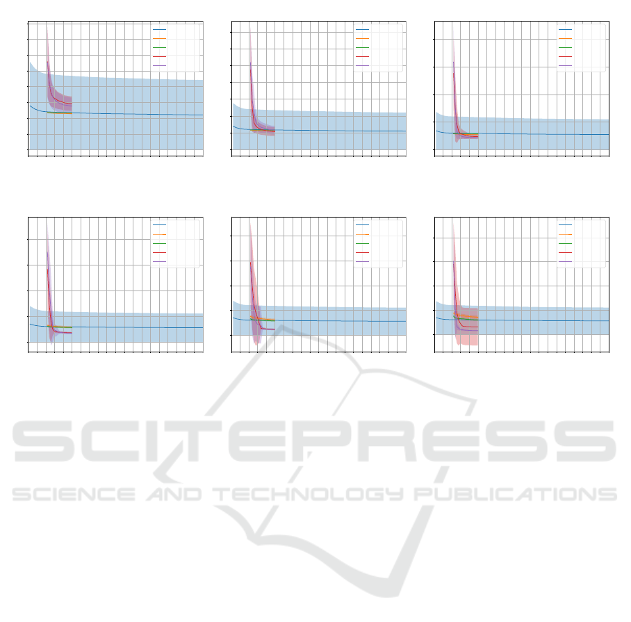
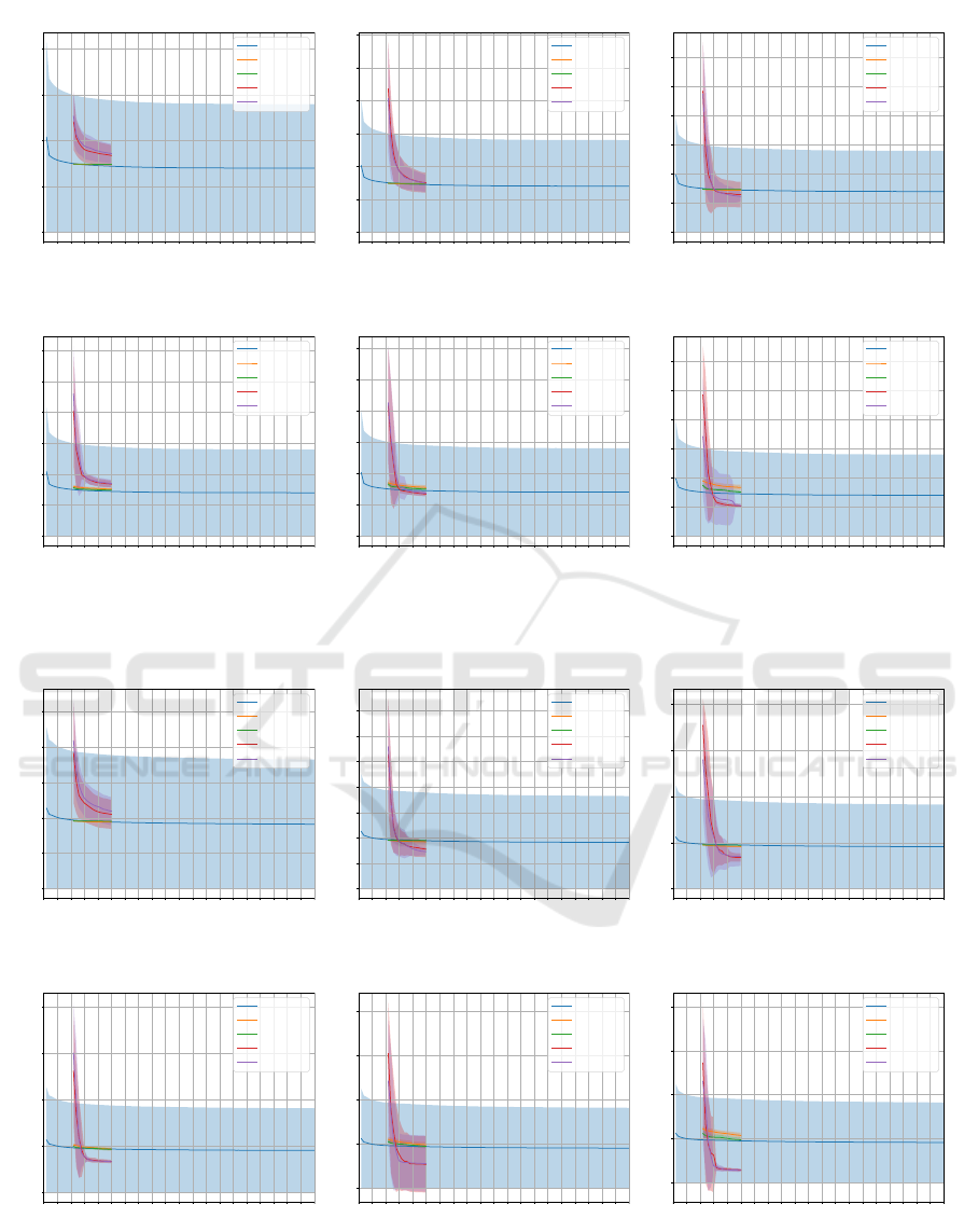
4.2 Convergence Analysis

Figures 2, 3, and 4 illustrate a comparison among

NBJS, JS, BH, and PSO convergence on MNIST, FM-

NIST, and KMNIST datasets for optimizing W pa-

rameter regarding 7×7 size images considering two ∆

conﬁgurations and 128, 256, and 512 hidden neurons,

respectively. In all cases in Figures 2, 3, and 4, the al-

gorithms obtained convergence similar to or superior

to the RBM convergence using 100 training epochs.

It is also noteworthy that the JS and NBJS techniques

surpassed the convergence of PSO and BH in all con-

ﬁgurations except for 128 hidden neurons as it can be

seen in Figures 2a, 3a, and 4a. It is worth mentioning

that the performance of all algorithms when ∆ = 1.0

in the MNIST dataset was shown to outperform when

∆ = 0.1.

However, a decreasing trend in the convergence of

JS and NBJS techniques, concerning images of size

7 × 7, can be observed in Figures 2a and 2b consider-

ing MNIST dataset, all conﬁgurations except for the

one shown in Figure 3d considering FMNIST dataset,

and, ﬁnally Figures 4a and 4b considering KMNIST

dataset.

5 CONCLUSION

This paper addressed increasing the reconstructability

of the RBM using metaheuristic optimization. The

idea is to pre-train an RBM model and ﬁne-tune both

the a bias and the W connection weights to minimize

the mean square error. Experiments were performed

on the MNIST, FMNIST, and KMNIST datasets with

three different image size settings: 7×7, 14×14, and

28 × 28.

The reported results demonstrated the feasibility

of using metaheuristic algorithms to ﬁne-tune con-

nection weights. The NBJS algorithm achieved er-

rors up to four times smaller than the baseline in

7 × 7. Fine-tuning the a parameter showed no sig-

niﬁcant inﬂuence on the models. Assuming that the

iterations of the metaheuristic algorithms are compu-

tationally equivalent to the computational cost of the

RBM training epochs, one can conclude that the meta-

heuristic algorithms achieve errors similar to or lower

than those of the RBM, requiring a lower number of

iterations.

Fine-Tuning Restricted Boltzmann Machines Using No-Boundary Jellyﬁsh

0 5 10 15 20 25 30 35 40 45 50 55 60 65 70 75 80 85 90 95 100

Iteration

Error

Delta: 0.1

Baseline

PSO

NBJS

0 5 10 15 20 25 30 35 40 45 50 55 60 65 70 75 80 85 90 95 100

Iteration

Error

Delta: 0.1

Baseline

PSO

NBJS

0 5 10 15 20 25 30 35 40 45 50 55 60 65 70 75 80 85 90 95 100

Iteration

Error

Delta: 0.1

Baseline

PSO

NBJS

(a) (b) (c)

0 5 10 15 20 25 30 35 40 45 50 55 60 65 70 75 80 85 90 95 100

Iteration

Error

Delta: 1.0

Baseline

PSO

NBJS

0 5 10 15 20 25 30 35 40 45 50 55 60 65 70 75 80 85 90 95 100

Iteration

Error

Delta: 1.0

Baseline

PSO

NBJS

0 5 10 15 20 25 30 35 40 45 50 55 60 65 70 75 80 85 90 95 100

Iteration

Error

Delta: 1.0

Baseline

PSO

NBJS

(d) (e) (f)

Figure 3: Convergence comparison on FMNIST dataset regarding 7 × 7 size images: (a) 128, (b) 256, and (c) 512 hidden

neurons with ∆ = 0.1, and (d) 128, (e) 256, and (c) 512 hidden neurons with ∆ = 1.0.

0 5 10 15 20 25 30 35 40 45 50 55 60 65 70 75 80 85 90 95 100

Iteration

Error

Delta: 0.1

Baseline

PSO

NBJS

0 5 10 15 20 25 30 35 40 45 50 55 60 65 70 75 80 85 90 95 100

Iteration

Error

Delta: 0.1

Baseline

PSO

NBJS

0 5 10 15 20 25 30 35 40 45 50 55 60 65 70 75 80 85 90 95 100

Iteration

Error

Delta: 0.1

Baseline

PSO

NBJS

(a) (b) (c)

0 5 10 15 20 25 30 35 40 45 50 55 60 65 70 75 80 85 90 95 100

Iteration

Error

Delta: 1.0

Baseline

PSO

NBJS

0 5 10 15 20 25 30 35 40 45 50 55 60 65 70 75 80 85 90 95 100

Iteration

Error

Delta: 1.0

Baseline

PSO

NBJS

0 5 10 15 20 25 30 35 40 45 50 55 60 65 70 75 80 85 90 95 100

Iteration

Error

Delta: 1.0

Baseline

PSO

NBJS

(d) (e) (f)

Figure 4: Convergence comparison on KMNIST dataset regarding 7 × 7 size images: (a) 128, (b) 256, and (c) 512 hidden

neurons with ∆ = 0.1, and (d) 128, (e) 256, and (c) 512 hidden neurons with ∆ = 1.0.

VISAPP 2023 - 18th International Conference on Computer Vision Theory and Applications

Regarding future work, we intend to test the per-

formance of the ﬁne-tuning in the bias of the invisible

layer b or even ﬁne-tune the parameters simultane-

ously, e.g. a and b.

ACKNOWLEDGEMENTS

The authors are grateful to FAPESP grants

#2013/07375-0, #2014/12236-1, #2019/07665-4,

#2019/18287-0, #2019/02205-5 and, #2021/05516-1,

and CNPq grants 308529/2021-9 and 427968/2018-6.

REFERENCES

Ackley, D., Hinton, G., and Sejnowski, T. J. (1988). A

learning algorithm for boltzmann machines. In Waltz,

D. and Feldman, J., editors, Connectionist Models and

Their Implications: Readings from Cognitive Science,

pages 285–307. Ablex Publishing Corp., Norwood,

NJ, USA.

Chou, J.-S. and Truong, D.-N. (2021). A novel metaheuris-

tic optimizer inspired by behavior of jellyﬁsh in ocean.

Applied Mathematics and Computation, 389:125535.

Hatamlou, A. (2018). Solving travelling salesman problem

using black hole algorithm. Soft Computing, 22:8167–

8175.

Hembecker, F., Lopes, H. S., and Godoy, W. (2007). Par-

ticle swarm optimization for the multidimensional

knapsack problem. In Beliczynski, B., Dzielinski,

A., Iwanowski, M., and Ribeiro, B., editors, Adaptive

and Natural Computing Algorithms, pages 358–365,

Berlin, Heidelberg. Springer Berlin Heidelberg.

Hinton, G. E. (2002). Training products of experts by min-

imizing contrastive divergence. Neural Computation,

14(8):1771–1800.

Hinton, G. E. (2012). A practical guide to training restricted

Boltzmann machines. In Montavon, G., Orr, G., and

Muller, K.-R., editors, Neural Networks: Tricks of the

Trade, volume 7700 of Lecture Notes in Computer

Science, pages 599–619. Springer Berlin Heidelberg.

Kennedy, J. and Eberhart, R. C. (2001). Swarm Intelli-

gence. Morgan Kaufmann Publishers Inc., San Fran-

cisco, USA.

Kuremoto, T., Kimura, S., Kobayashi, K., and Obayashi,

M. (2012). Time series forecasting using restricted

boltzmann machine. In International Conference on

Intelligent Computing, pages 17–22. Springer.

Papa, J. P., Rosa, G. H., Costa, K. A. P., Marana, A. N.,

Scheirer, W., and Cox, D. D. (2015). On the model

selection of bernoulli restricted boltzmann machines

through harmony search. In Proceedings of the

Genetic and Evolutionary Computation Conference,

pages 1449–1450, New York, NY, USA. ACM.

Papa, J. P., Scheirer, W., and Cox, D. D. (2016). Fine-tuning

deep belief networks using harmony search. Applied

Soft Computing, 46:875–885.

Passos, L. A., de Souza Jr, L. A., Mendel, R., Ebigbo, A.,

Probst, A., Messmann, H., Palm, C., and Papa, J. P.

(2019). Barrett’s esophagus analysis using inﬁnity re-

stricted Boltzmann machines. Journal of Visual Com-

munication and Image Representation.

Wang, K.-P., Huang, L., Zhou, C.-G., and Pang, W. (2003).

Particle swarm optimization for traveling salesman

problem. In Proceedings of the 2003 International

Conference on Machine Learning and Cybernetics

(IEEE Cat. No.03EX693), volume 3, pages 1583–

1585.

Wilcoxon, F. (1945). Individual comparisons by ranking

methods. Biometrics Bulletin, 1(6):80–83.

Fine-Tuning Restricted Boltzmann Machines Using No-Boundary Jellyﬁsh