Constraint-Based Filtering and Evaluation of CSP Search Trees

Maximilian Bels, Sven L

ofﬂer and Ilja Becker and Petra Hofstedt

Programming Languages and Compilers Group, Brandenburg University of Technology,

Konrad-Wachsmann-Allee 5, Cottbus, Germany

ﬂ

Keywords:

Constraint Programming, Finite-Domain Constraint Satisfaction Problem, CSP, Search Tree,

Constraint-Based Filtering.

Abstract:

Using Constraint Programming (CP) real world problems can be described conveniently in a declarative way

with constraints in a so-called constraint satisfaction problem (CSP). Finite domain CSPs (FD-CSPs) are one

form of CSPs, where the domains of the variables are ﬁnite. Such FD-CSPs are mostly evaluated by a search

nested with propagation, where the search process can be represented by search trees. Since search can quickly

become very time-consuming, especially with large variable domains (solving CSPs is NP-hard in general),

heuristics are used to control the search, which in many cases — depending on the problem — allow to achieve

a performance gain. In this paper, we present a new method for ﬁltering and evaluating search trees of FD-

CSPs. Our new tree ﬁltering method is based on the idea of formulating and evaluating ﬁlters as constraints

over FD-CSP search trees. The constraint-based formulation of ﬁlter criteria proves to be very ﬂexible. Our

new technique was integrated into the Visual Constraint Solver (VCS) tool, which allows the solution process

of CSPs to be followed interactively and step by step through a suitable visualization.

1 INTRODUCTION

Finite-Domain Constraint Satisfaction Problems (FD-

CSPs) are evaluated by search nested with propaga-

tion. Search heuristics control the search. They affect

the structure of the search trees of CSPs and can, thus,

inﬂuence the performance of CSP evaluation. Our

aim is to compare, review and better understand the

impact of search heuristics.

Search trees can quickly become extraordinarily

large. At the same time, for a comparison or review,

one only wants to consider certain sections of the tree.

Thus, we want to be able to formulate and evalu-

ate criteria for particularly interesting sets of search

nodes and parts of search trees.

In this paper, we present a new method for formu-

lating criteria and ﬁltering and evaluating search trees

of FD-CSPs. The main idea is to formulate the search

tree ﬁlters themselves as CSPs. Data of nodes and

their relations in subtrees can be described very ﬂex-

ibly by variables and constraints. A constraint solver

can be used to evaluate the ﬁlter CSPs and provide

optimized solutions.

Our new method was integrated into the Visual

Constraint Solver (VCS). VCS is a tool for the visu-

alization of FD-CSP evaluation developed at the Pro-

gramming Languages and Compilers group (PSCB)

at BTU Cottbus-Senftenberg. VCS takes as in-

put MiniZinc (MiniZinc, 2022) programs describing

CSPs and allows to visualize the static CSP as well as

the solution process by a search tree and log ﬁles.

Related Work. Some tools for the visualization of

CSPs and search trees have been documented in the

literature, among them a constraint graph viewer for

the platform G12 (Mak, 2022), DPViz (for SAT prob-

lems) (Sinz and Dieringer, 2005), CPViz (Simonis

et al., 2010) and DrawCSP (Li and Epstein, 2010).

These tools are typically designed for speciﬁc con-

straint languages or solvers, they often visualize CSP

networks, but do not visualize the search trees, and

even if so, they do not allow to deﬁne ﬁlters on trees

as ﬂexible as our method does. In contrast, VCS

works on MiniZinc models which are solver inde-

pendent, is very ﬂexible in the deﬁnition of search

tree ﬁlters, supports the interactive visualization of

search trees and node properties and even allows to

compare different search strategies at the same time.

Moreover, VCS supports the visualization of (multi-

dimensional) arrays, which is a further unique feature

of our tool.

The paper is structured as follows: Section 2 re-

calls basic terms and deﬁnitions of the area of con-

220

Bels, M., Löfﬂer, S., Becker, I. and Hofstedt, P.

Constraint-Based Filtering and Evaluation of CSP Search Trees.

DOI: 10.5220/0011641100003393

In Proceedings of the 15th International Conference on Agents and Artiﬁcial Intelligence (ICAART 2023) - Volume 3, pages 220-227

ISBN: 978-989-758-623-1; ISSN: 2184-433X

 2023 by SCITEPRESS – Science and Technology Publications, Lda. Under CC license (CC BY-NC-ND 4.0)

straint programming. We introduce the notions of

ﬁlter criteria and ﬁlter models in Section 3. Follow-

ing, Section 4 discusses technical and implementation

details of our constraint-based approach to ﬁltering

search trees as well as the visualization inside our tool

VCS. Section 5 demonstrates the modelling of further

useful ﬁlters. Finally, in Section 6 we conclude the

paper and give directions of future research.

2 CONSTRAINT

PROGRAMMING

This section provides basic concepts and deﬁni-

tions of constraint programming (based on (Dechter,

2003)).

Deﬁnition 1 (constraint). Let X be a set of variables.

A constraint c = (X

′

, R) is a relation R over a subset

′

of the variables of X, i.e. X

′

⊆ X.

The relation R of a constraint c = (X,R) repre-

sents a subset of the Cartesian product of the domain

values D

× ... × D

of the corresponding variables

, ..., x

∈ X. It can be given explicitly by the con-

cerning value tuples or implicitly by a mathematical

description.

Deﬁnition 2 (CSP). A constraint satisfaction problem

(CSP) is deﬁned as a triple P = (X, D,C), where

• X = {x

, . . . , x

} is a set of variables,

• D = {D

, . . . , D

} is a corresponding set of do-

mains, i.e. D

is the domain of x

, and

• C = {c

, . . . , c

} is a set of constraints.

In the following, we only consider ﬁnite domain-

CSPs (FD-CSPs) (and write CSP), where the variable

domains are ﬁnite.

Example 1. The n-queens problem aims to place n

queens on an n × n-chess board such that the queens

do not attack each other. For example, for the 5-

queens instance we can give a CSP P = (X, D,C) as

follows:

• X = {q

, . . . , q

} are variables to represent the

queens, such that queen q

is placed on column

• D = {D

, . . . , D

= . . . = D

= {1, 2, 3, 4, 5}}

are the domains of the variables q

; they represent

the row numbers on the board,

• C = {alldifferent({q

, . . . , q

}),

alldifferent({q

+ i | i ∈ {1, . . . , n}}),

alldifferent({q

− i | i ∈ {1, . . . , n}})}

are the constraints to ensure that the queens can-

not threaten each other. Here, the ﬁrst constraint

says that all q

should be different, this ensures

Figure 1: A solution of the 5-queens problem.

distinct rows for the queens. The other two con-

straints determine distinct diagonals. At this, the

alldifferent constraint is a so-called global con-

straint which ensures that the values of all in-

cluded variables are distinct.

A solution of a CSP is an instantiation of all its

variables with values from their domains, that satis-

ﬁes all the constraints (Dechter, 2003). For example,

the 5-queens problem has 10 solutions, including e.g.

= 1, q

= 3, q

= 5, q

= 2, q

= 4 as illustrated by

Figure 1.

The search for solutions of a CSPs is realized

by constraint solvers which use backtracking-based

depth-ﬁrst search. To speed-up the search, it is inter-

leaved with constraint propagation steps. Each indi-

vidual constraint describes a set of allowed tuples. By

propagating a constraint one can constrain the search

space locally, i.e. values that do not satisfy a con-

straint and are therefore not involved in any solution,

are removed from the search space. The solver per-

forms such propagation steps in alternation with vari-

able instantiation during search. This process is de-

scribed in detail e.g. in (Dechter, 2003; Marriott and

Stuckey, 1998).

Furthermore, search heuristics are used in the

search for solutions of CSPs. We distinguish between

variable ordering and value ordering heuristics (van

Beek, 2006).

Variable ordering heuristics decide which vari-

able is next instantiated to a value during the

backtracking-based search. Different variable heuris-

tics typically yield differently structured search trees.

The goal of these heuristics are strong domain restric-

tions early on and narrow search trees. This can be

achieved e.g. with the ﬁrst-fail heuristic, where vari-

ables with the smallest domains are chosen ﬁrst. With

a similar intention, the most-constraint heuristic ﬁrst

takes variables that are attached to many constraints

of the given CSP.

Value ordering heuristics decide which value a

previously selected variable is assigned. Value heuris-

tics do not affect the general structure of the search

tree, but they lead to a reordering of the sub trees of

a search tree. This is particularly interesting and can

Constraint-Based Filtering and Evaluation of CSP Search Trees

221

be advantageous if only a ﬁrst solution or best solu-

tion(s) are sought or when parallel search or no-good

learning is applied.

Both kinds of heuristics manipulate the search tree

and thus can signiﬁcantly affect the time required in

the solution process. For this reason, it is important to

evaluate different search heuristics in order to predict

a good or potentially best strategy for solving a given

problem as quickly as possible.

Constraint solvers, such as the Choco

solver (Choco, 2022), provide a number of vari-

able and value ordering heuristics. However, the

appropriate choice of the heuristics is the responsibil-

ity of the user.

3 DEFINING FILTER MODELS

Our aim is to review and evaluate the performance of

search heuristics by assessing and comparing search

trees of CSPs. This is realized by ﬁlters on search tree

node sets, expressed themselves as CSPs and evalu-

ated by a constraint solver.

In this section, we ﬁrst recall search trees. Next,

we explain the notions and usages of properties of

search tree nodes and ﬁlter criteria on sets of such

nodes. On top of these, we deﬁne the notion of a ﬁl-

ter model which allows to express constraints on node

sets and subtrees of search trees.

3.1 Search Trees

Deﬁnition 3 (search tree). Let a CSP P = (X , D,C)

be given. A search tree for P is a tree T, whose nodes

represent P enriched by instantiations to subsets of

X. For every node in T , we assume that consistency

enforcement has been applied. The root of T stands

for P (after consistency enforcement and with no fur-

ther variable instantiation). A child of a node n is an

extension of the instantiation of n for exactly one vari-

able v of X , where the size of the remaining domain of

v is greater than one. A leaf is either a solution of P

or inconsistent (noticed by f ail).

Example 2. We consider a CSP P = (X , D,C)

with X = {x, y, z}, D = {D

= D

= {0, 1, 2}, D

{0, 1, 2, 3}} and C = {x < y, z = x + y}. A search tree

for P is given in Figure 2.

The root node stands for the original problem P,

where propagation of the constraints has already been

performed and, thus, the domains of the variables

have been narrowed. E.g. from x < y follows, that

x cannot be 2 and y cannot be 0.

P has two child nodes P

and P

. P

represents P,

where we assigned 0 to x. These instantiations are no-

ticed on the edges between the parent and child nodes.

By further propagation for consistency enforcement,

also the domains of the other variables may be af-

fected, for P

e.g. 3 is removed from the domain of

Finally, for P the solution process reveals three so-

lutions as shown in the leaf nodes of the tree.

3.2 Node Properties and Filter Criteria

To describe, to ﬁlter, and to cut out parts of a search

tree with certain interesting properties with respect to

the solution process we use properties of the search

tree nodes and call them node properties. Since the

search tree is dynamically generated resp. traversed

during the solution process by backtracking search,

node properties are gained dynamically during search.

We identiﬁed certain relevant node properties. At

this, we take as basis a left-to-right backtrack search

and consider properties which appear caused by the

course of the search and the tree structure (properties

a-i) as well as properties of the CSP and variable in-

stantiations at the corresponding node (properties j-k).

The node properties of node n include the following

(this list is not exclusive and can even be extended by

the user):

a the discovery index n

∈ N of the node n in the

left-to-right backtracking order of the tree (the

root node has discovery index 1),

b the number n

solutions

∈ N of solutions found so far

(during backtracking search, including n), when

the node n is reached in the tree,

c the number n

leafs

∈ N of leaf nodes (solutions

and dead ends, including n) found so far during

search,

d the depth n

depth

∈ N of the node in the search tree,

e the index n

parentId

∈ N ∪ {−1} of the parent of

node n (or −1 in case n is the root),

f a truth value (0 for false, 1 for true) n

isLeft

to ex-

press, whether n is a left-most child of it’s parent

(or 1 in case n is the root),

g the index n

lastLeftParentId

∈ N of the closest left an-

cestor of n, that is, the closest ancestor where

isLeft

is 1,

h a truth value (0 for false, 1 for true) n

isSolution

to ex-

press, whether n represents a solution (leaf node),

i a truth value (0 for false, 1 for true) n

isContradiction

to express, whether n is a contradiction (leaf

node),

j the size n

a,domainSize

∈ N of the domain of a certain

variable a,

ICAART 2023 - 15th International Conference on Agents and Artiﬁcial Intelligence

222

with x ∈ {0, 1}, y ∈ {1, 2}, z ∈ {1, 2, 3}

x ∈ {0}, y ∈ {1, 2}, z ∈ {1, 2}

1,1

x ∈ {0}, y ∈ {1}, z ∈ {1}

y = 1

1,1

x ∈ {0}, y ∈ {2}, z ∈ {2}

y = 2

x = 0

x ∈ {1}, y ∈ {2}, z ∈ {3}

x = 1

Figure 2: Search tree for Example 2.

k the domain value of a variable a, in case that the

variable is ﬁnally instantiated n

a,instantiatedTo

∈ D

(otherwise undeﬁned).

To analyse, to visualize, and to compare search

trees to better understand search behaviour we want

to ﬁlter search trees and nodes by certain criteria. We

use the above explained node properties, either di-

rectly or for the formulation of complexer constraints

over several nodes or parts of a search tree.

We give typical deﬁnitions of potentially interest-

ing ﬁlter criteria for node sets and subtrees. Later on,

we will see that the user of our system will be able to

deﬁne such criteria and constraints by himself.

A Variable instantiations. A ﬁrst, simple ﬁlter

goal is to ﬁnd the positions or nodes in a search

tree, where a speciﬁc variable a is assigned a spe-

ciﬁc value v

. Find a node n, such that holds:

a,instantiatedTo

= v

B Number of nodes visited to ﬁnd a certain number

of solutions. As well, one can be interested to

ﬁnd out, how many nodes have been visited until

m solutions were found. Determine a node n, such

that holds: n

solutions

= m. The discovery index n

of n is the searched number of visited nodes.

There are also clearly more complex descriptions

possible, which refer to subtrees or node sets, e.g. so-

lution density or domain reduction.

C Solution density. The solution density describes

the proportion of solutions in the set of leafs in a

certain region of the search tree.

Deﬁnition 4 (solution density). The solution den-

sity den(n

, n

) of a set of all nodes visited during

search between the nodes n

(visited ﬁrst) and n

(visited last) is deﬁned by:

den(n

, n

) :=

solutions

− n

solutions

leafs

− n

leafs

whereby n

solutions

≤ n

solutions

, n

leafs

≤ n

leafs

With additional constraints on the nodes, one can

search for appropriate nodes n

and n

which

determine a search tree. In this way, one can

search for subtrees with a high/low solution den-

sity which may indicate areas in the tree, where

the used heuristics are particularly effective/inef-

fective.

D Domain reduction. The domain reduction de-

scribes the strength of the reduction of a variable

domain in the progression of the search between

two nodes in the tree.

Deﬁnition 5 (domain reduction). The domain re-

duction red(n

, n

, a) by search during tree traver-

sal between the nodes n

and n

and with respect

to variable a is deﬁned by:

red(n

, n

, a) := 1 −

a,domainSize

At this, we assume, that n

is a node in a subtree

with root n

. Thus, also n

a,domainSize

≤ n

a,domainSize

holds.

With domain reduction we can observe the inﬂu-

ence of a heuristics on the domain of certain vari-

ables in search trees, e.g. we can ﬁlter for parts,

where the domain is reduced by e.g. 50 %. With

additional constraints on the indices of the two

nodes n

and n

we can ﬁnd positions in the tree

with a fast/slow domain reduction for certain vari-

ables.

Again, and as for the ﬁlter properties holds: The

set of ﬁlter criteria is extendable and programmable

by the user of our system.

3.3 Filter Models

Depending on the application case, one may be inter-

ested in different node properties and evaluation cri-

teria. E.g. consider a lecture in Constraint Program-

ming, where the instructor wants to explain the idea of

Constraint-Based Filtering and Evaluation of CSP Search Trees

223

search and search trees in general. In this case, it may

be sensitive to focus on simple properties like node

indexes, node depth in a search tree, or the number of

decisions taken during search up to a certain node. In

contrast, if one wants to optimize a search heuristics

for a certain problem class, more complex, composed

criteria (as e.g. in Deﬁnition 4) might be important.

To allow a deﬁnition of criteria as individually and

freely as possible, we decided to deﬁne and handle

themselves as CSPs. Such CSP models of criteria are

called ﬁlter CSPs or ﬁlter models in the following.

A ﬁlter model is a CSP F modeled around an orig-

inal CSP P (i.e. the problem CSP) and its search tree.

One the one hand, a ﬁlter model F may contain ad-

ditional variables and constraints to enhance the origi-

nal CSP P. This may help to shrink a given problem to

be able to consider partial aspects of P, e.g. consider

P, where a certain variable instantiation is somehow

ﬁxed. On the other hand (and more interestingly), the

ﬁlter CSP F describes constraints over the nodes of

the search tree. Thus, the variables of F represent tree

nodes and tree node properties. Accordingly, the do-

main D

of such a search node variable n is the set

of all search tree nodes (represented by a unique node

index), the domain D

n,prop

of a property variable of

a tree node is the set of the possible values of such

a property. Finally, constraints of F describe search

node sets and constraints on them.

Deﬁnition 6 (ﬁlter model). Given a problem CSP P =

(X, D,C). A ﬁlter CSP (or ﬁlter model) F = (X

∪

, D

∪ D

) consists of

• a set X

of variables with ﬁnite domains D

(to

enhance the original CSP P),

• a set X

of variables with ﬁnite domains D

(to

describe search tree nodes and search tree node

properties)

• a set C

of constraints over X

∪ X

∪ X.

While the set C

of constraints may contain fur-

ther model constraints on P (as explained above), it

primarily consists of constraints on search tree nodes.

These constraints are used to specify node sets of a

search tree by specifying desired node properties and

relations between the nodes and node properties.

Example 3. Let the CSP P from Example 1 describ-

ing the 5-queens problem be given. A ﬁlter model

F = (X

, D

) with

• X

= {n, n

isSolution

• D

= {D

, D

isSolution

= B }, where D

is the set of

all search tree nodes (represented by unique in-

dexes), and

• C

= {n ≤ 30, n

isSolution

= true}

speciﬁes a ﬁlter which provides all solutions within

the ﬁrst 30 search tree nodes visited during backtrack-

ing search.

More complex examples, including the search for

subtrees with restrictions on the domain reduction and

solution density, are given in Section 5.

Since the original problem CSP P is an FD-CSP,

it is ensured that all search trees of P are ﬁnite. Thus,

the number of search tree nodes and their concern-

ing properties is ﬁnite as well. However, in practice,

we do not know in advance, the concrete nodes of a

proper search tree nor their property values because a

search tree is generated dynamicall during the evalu-

ation of the original problem CSP P. Thus, while we

are able to formulate the needed variables and con-

straints on them for the ﬁlter CSP F, we cannot pro-

vide their property values in advance. In this way,

the ﬁlter CSP F is initially incomplete. During search

additional constraints for deﬁning the property values

of the nodes must be added to F. This is discussed in

more detail in the following section.

4 FILTER IMPLEMENTATION

The Visual Constraint Solver (VCS) is a tool for the

visualization of FD-CSPs and their evaluation, devel-

oped at BTU Cottbus-Senftenberg in a series of bach-

elor/master theses (Buckenauer, 2019; Reda, 2020;

Bels, 2022). As input, VCS takes MiniZinc programs

which specify CSPs. MiniZinc (Stuckey et al., 2020;

MiniZinc, 2022) is a high-level, solver-independent

constraint modeling language whose constraint mod-

els are compiled via the intermediate language Flat-

Zinc into other constraint programming languages

such as Choco (Choco, 2022). Choco is a Java li-

brary for constraint solving and it is used inside VCS

to solve FD-CSPs.

Filter models (as described in Section 3) are our

new extension of VCS. Observe, that they are just

CSPs on search tree nodes and their properties. Thus,

the main idea of their implementation is to represent

them by constraint models and to handle them by con-

straint solvers. This yields an extended workﬂow:

Filter models are deﬁned just like problem CSP

models using MiniZinc. They are as well compiled

into a Choco constraint model F

choco

via FlatZinc.

When the original problem CSP P

choco

is solved by

the Choco solver, additional information about the

nodes and node properties is collected and used to ex-

tend the Choco ﬁlter model. The resulting enhanced

ﬁlter constraint model F+

choco

is again solved by the

Choco solver. Its solutions are used to enhance and

decorate the visualization of the solutions of P

choco

ICAART 2023 - 15th International Conference on Agents and Artiﬁcial Intelligence

224

1 i nc lu de " all dif fe ren t . m z n ";

2 int : n = 5;

3 % n is the nu m be r of quee ns

4 a rra y [1.. n ] of var 1. . n : q ;

5 % quee n in colu mn i is in row q [i ]

6 co ns tr ain t al l dif fer e nt ( q);

7 % all que en s in dis ti nc t ro w s an d

...

8 co ns tr ain t al ld iff e ren t ([ q [i] + i |

i in 1. . n ]) ;

9 co ns tr ain t al ld iff e ren t ([ q [i] - i |

i in 1. . n ]) ;

10 % ... di st in ct d ia gon a ls

11 s olv e sa ti sf y ;

Listing 1: A MiniZinc model of the 5-queens problem.

1 var int : n_id ;

2 var int : n _i sSo lu tio n ;

3 co ns tr ain t n_ i d <= 3 0 ;

4 co ns tr ain t n_ is Sol u tio n = 1;

5 s olv e sa ti sf y ;

Listing 2: A ﬁlter for all solutions within the ﬁrst 30 nodes

visited during backtracking search.

the VCS tool by highlighting node sets satisfying the

ﬁlter CSP.

Listing 1 gives an example of a MiniZinc CSP

model. It speciﬁes the 5-queens problem CSP P =

(X, D,C) from Example 1. After an import of the

global alldifferent constraint from the MiniZinc

libraries (Line 1), the variables q[1] to q[5] (orga-

nized in an array) with their domain values 1 to 5

(Lines 2,4) are deﬁned. In Lines 6-9 the constraints

of set C are given as above. Line 11 initiates the solu-

tion process.

The script in Listing 2 is an example of a ﬁlter

model in MiniZinc which corresponds to Example 3.

It declares a search node n with unique identiﬁer n id

and property n isSolution. The constraints ensure

that the desired node is a solution (n isSolution =

1) and is visited within the ﬁrst 30 nodes (n id <=

30). The last line instructs the solver to search for

a solution that satisﬁes all constraints. Notice, that

properties must always be given in conjunction with a

ﬁlter node index and may require to specify an associ-

ated variable in addition to that (here n isSolution).

Visualization of Filter Results. When assessing a

CSP and its solution process using VCS the user can

load problem CSPs P and ﬁlter models F. Besides

If there are no nodes satisfying a ﬁlter model, the

search tree is shown by VCS just as before and without ad-

ditional decorations.

he can choose between variable and value ordering

heuristics provided by Choco. The problem CSP can

be solved step-wise and ﬁlter models can be applied

interleaved.

Figure 3 shows a cut-out of the search tree of the

5-queens CSP from Example 1 and Listing 1 in VCS.

We used the ﬁlter given in Listing 3 (to be explained

in Section 5 in more detail). This ﬁlter model identi-

ﬁes parts of the tree with a solution density (cf. Deﬁ-

nition 4) of at least 50%.

In the shown case, the search tree nodes with in-

dices 16-22 include 4 leafs, where 2 of them (nodes

17 and 19) are solutions (solution density is 50%).

Green nodes represent solutions of the problem

CSP P, red nodes stand for failing subtrees. Yellow

coloured nodes represent a ﬁlter result. It is possi-

ble to switch step-by-step between the several ﬁlter

results, here subtrees satisfying the ﬁlter model. The

user of VCS can assess the ﬁltered node data by click-

ing on a search tree node. Then a window opens

and shows the node properties, e.g. at node 17 we

see a solution of the 5-queens problem. (Notice, the

X INTRODUCED i variable names result from the Flat-

Zinc conversion of the queens array inside VCS and

stand for the queens q

i+1

, i.e. X INTRODUCED 0 for

, X INTRODUCED 1 for q

and so on).

5 APPLICATION EXAMPLES

Now, let us consider further examples of ﬁlter scripts

which shall help to asses search heuristics. They are

written in MiniZinc as before and provided as input

for VCS together with a problem CSP P.

Listing 3 shows a ﬁlter speciﬁcation for subtrees

with a high solution density according to Deﬁnition 4.

In Lines 1 and 6, two search tree nodes n1 and n2

are declared. Node n1 is the root of the to be ﬁltered

subtree, node n2 the subtree’s rightmost leaf. For the

actual deﬁnition of the ﬁlter criterion in Line 20, we

need certain node properties gained with the code in

the Lines 2-5 and 7-12. Lines 15-19 specify the sub-

tree structure (for the meaning of n

lastLeftParIdx

and n isLeft see the node properties f and g in Sec-

tion 3), mainly by stating that n1 must be the root

of a subtree and n2 must be a descendant of n1 and a

right-most leaf node (a solution or contradiction). The

value of n leafs is the number of leafs (solutions and

fails) visited so far during the search process. Prop-

erty n solutions gives the number of solutions seen

so far in the search process. The ﬁlter criterion of a

high solution density is deﬁned in Line 20, where we

use a density threshold of 50% (Line 13). Line 21

initiates the solution process, i.e. the ﬁlter evaluation.

Constraint-Based Filtering and Evaluation of CSP Search Trees

225

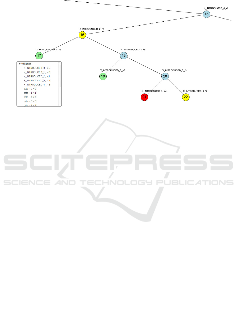
Figure 3: Filtering a search tree for subtrees with a solution density of at least 50%.

1 var int : n1 _ id ;

2 var int : n 1_l ast Le ft P arI dx ;

3 var int : n 1_ is Le ft ;

4 var int : n 1_ le af s ;

5 var int : n 1_ sol ut ion s ;

6 var int : n2 _ id ;

7 var int : n 2_l ast Le ft P arI dx ;

8 var int : n 2_ is Le ft ;

9 var int : n 2_ le af s ;

10 var int : n 2_ sol ut ion s ;

11 var int : n 2_ isS olu ti on ;

12 var int : n 2_i sCo ntr ad ic t io n ;

13 int : pctg = 50;

14 % min im um s o luti on p er cen ta ge

15 co ns tr ain t n 1_i d < n 2_i d ;

16 co ns tr ain t n 2_i s Lef t = 0;

17 co ns tr ain t ( int_ eq ( n1_ id ,

n2 _la st Le f tPa rId x ) \/

18 ( n1_ is Lef t = 0 /\ i nt _e q (

n2 _ last Le ftPa rI dx ,

n1 _la st Le f tPa rId x )) );

19 co ns tr ain t (( n 2_i sS olu ti on = 1) \/

( n 2 _i s Con tra dic tio n = 1) );

20 co ns tr ain t ( n2 _ sol ut ion s -

n1 _s olu ti ons ) * 100 di v (

n2 _ le afs - n 1 _l eafs ) >= pctg ;

21 s olv e sa ti sf y ;

Listing 3: Filtering subtrees with high solution density.

Listing 4 is a ﬁlter for ﬁnding nodes which per-

form a strong domain reduction. First, in Lines 1 and

3, the tree nodes n1 and n2 are declared. The property

X INTRODUCED 2 dom provides the domain size of

a variable X INTRODUCED 2 when node n is reached.

The index of the parent node of a node is speciﬁed by

1 var int : n1 _ id ;

2 var int : n 1_X _IN TRO DUC ED_ 2_d om ;

3 var int : n2 _ id ;

4 var int : n 2_ par en tI d ;

5 var int : n 2_X _IN TRO DUC ED_ 2_d om ;

6 int : pctg = 30;

7 co ns tr ain t i nt _e q ( n 2_ p ar e nt Id ,

n1_i d ) ;

8 co ns tr ain t 100 - (

n2 _X_ INT ROD UCE D_2 _do m * 1 0 0 div

n1 _X_ INT ROD UCE D_2 _do m ) >= pc t g ;

9 s olv e sa ti sf y ;

Listing 4: Filtering subtrees with a strong domain reduction.

n parentId. The constraint in Line 7 ensures that n1

is the direct parent node of node n2. In Line 8 the cri-

terion of domain reduction is determined according to

Deﬁnition 5 and compared against a certain threshold

value (here 30%, Line 6).

The extension of VCS by our new node ﬁlter-

ing mechanism allows to debug and analyze search

heuristics in detail. When the user wants to com-

pare two search trees (and thus get insights about dif-

ferences of search heuristics), he can deﬁne problem

oriented criteria based on node properties, solve his

problem CSP P and ﬁlter the search trees by the ﬁlter

criteria deﬁned in a ﬁlter CSP F. VCS supports a vi-

sualization of the ﬁltered node sets and subtrees and

provides further data on the tree nodes including the

node properties.

ICAART 2023 - 15th International Conference on Agents and Artiﬁcial Intelligence

226

6 CONCLUSION

In this paper we introduced a new method for the as-

sessment and comparison of search heuristics at the

evaluation of FD-CSPs. For this, we deﬁne ﬁlter

model CSPs, which describe criteria to ﬁlter subtrees

of search trees with speciﬁc properties. The com-

parison and systematic analysis of CSP search trees

can help to understand the preconditions for good

and successful heuristics for speciﬁc applications and

in general and may help to improve dynamic search

heuristics. At this, our main observation was that such

ﬁlters for search trees are themselves just again CSPs.

Thus, we realized a method to deﬁne ﬁlter CSPs and

to handle these by a constraint solver which makes

our method very ﬂexible.

Our new method was integrated into the Visual

Constraint Solver tool, which allows to present CSPs

and the solution process interactively, step-by-step

through a suitable visualization. With the extension

by ﬁlter models, VCS now became a tool for debug-

ging CSPs, comparing search strategies, and under-

standing search in detail.

Future Work. Currently, VCS is in a prototypical

implementation state; in the future we will further im-

prove and optimize this tool, its workﬂow and expand

its application area. Considering the implementation

of the ﬁltering feature, improvement is needed for

handling large CSPs with high numbers of variables

and constraints together with (more complex) ﬁlters.

This combination yields a growth of constraints and

data and can quickly become a memory bottleneck.

We need to investigate ways of handling this prob-

lem, e.g. by more appropriate data structures, internal

constraint representations, and early node set pruning.

Another direction of future work is to provide the

user with descriptions of tree patterns for an easier

speciﬁcation of ﬁlter CSPs (e.g. for the a pattern for

subtrees like Lines 15-19 in Listing 3).

Furthermore, currently only the predeﬁned search

heuristics of the Choco solver are taken into consid-

eration as search heuristics. An extension of our ap-

proach to other search strategies like domain splitting

is desirable.

REFERENCES

Bels, M. (2022). Evaluation und Visualisierung von

Entscheidungsb

aumen und Variablen- und Wer-

tauswahlheuristiken im Visual Constraint Solver.

Bachelor Thesis, BTU Cottbus-Senftenberg.

Buckenauer, D. (2019). Redesign des Tools Visual Con-

straint Solver (VCS). Bachelor Thesis, BTU Cottbus-

Senftenberg.

Choco (2022). Choco - an open-source java library for con-

straint programming. https://choco-solver.org/. last

visited 2022-10-14.

Dechter, R. (2003). Constraint Processing. Elsevier Mor-

gan Kaufmann.

Li, X. and Epstein, S. L. (2010). Visualization for structured

constraint satisfaction problems. In Visual Represen-

tations and Reasoning, Papers from the 2010 AAAI

Workshop, Atlanta, Georgia, USA, July 11, 2010.

AAAI.

Mak, A. (2022). Constraint graph visualization. http:

//users.cecs.anu.edu.au/

∼

anthonym/cgv.pdf. last vis-

ited 2022-10-14.

Marriott, K. and Stuckey, P. (1998). Programming with

Constraints. An Introduction. The MIT Press.

MiniZinc (2022). The constraint modeling language mini-

zinc. https://www.minizinc.org/. last visited 2022-10-

14.

Reda, A. (2020). Visualisierung von Arrays in

Constraint-Satisfaction-Problemen. Master Thesis,

BTU Cottbus-Senftenberg.

Simonis, H., Davern, P., Feldman, J., Mehta, D., Quesada,

L., and Carlsson, M. (2010). A generic visualiza-

tion platform for CP. In Cohen, D., editor, Principles

and Practice of Constraint Programming - CP 2010,

volume 6308 of Lecture Notes in Computer Science,

pages 460–474. Springer.

Sinz, C. and Dieringer, E. (2005). Dpvis - A tool to visual-

ize the structure of SAT instances. In Bacchus, F. and

Walsh, T., editors, Theory and Applications of Satis-

ﬁability Testing - SAT 2005, volume 3569 of Lecture

Notes in Computer Science, pages 257–268. Springer.

Stuckey, P. J., Marriott, K., and Tack, G. (2020). Mini-

Zinc Handbook. https://www.minizinc.org/doc-2.6.3/

en/index.html, last visited 2022-10-14.

van Beek, P. (2006). Backtracking search algorithms. In

Rossi, F., van Beek, P., and Walsh, T., editors, Hand-

book of Constraint Programming, chapter 4, pages

85–134. Elsevier.

Constraint-Based Filtering and Evaluation of CSP Search Trees

227