Counterfactual Explanations for

Workforce Scheduling and Routing Problems

Mathieu Lerouge

1,3 a

, C

eline Gicquel

2 b

, Vincent Mousseau

1 c

and Wassila Ouerdane

1 d

MICS CentraleSupelec, Universite Paris-Saclay, Gif-sur-Yvette, France

LISN, Universite Paris-Saclay, Gif-sur-Yvette, France

DecisionBrain, Paris, France

Keywords:

Workforce Scheduling and Routing Problem, Integer Linear Programming, Counterfactual Explanation.

Abstract:

End-users of system solving combinatorial optimization problems such as the Workforce Scheduling and

Routing Problem usually do not have the necessary background for understanding the reasons which has lead

the system to output speciﬁc solutions and may have questions about them, especially questions about non-

expected facts observed in the solutions. Developing techniques to automatically generate explanations in

response to end-users questions would then help enhancing their understanding of the results and preserve

their trust in the system. In this paper, we propose a new mathematical programming-based approach to

compute counterfactual explanations in response to end-users’ questions. Such explanations emphasize the

few changes that may be operated on the instance data for obtaining solutions corresponding to the end-users’

expectations.

1 INTRODUCTION

The Workforce Scheduling and Routing Problem

(WSRP) is a Combinatorial Optimization (CO) prob-

lem which involves assigning geographically dis-

persed tasks to members of a mobile workforce and

creating a pair of route and schedule for each of these

members. It occurs in various contexts like home

health care (e.g. (Euchi et al., 2022)) or technical ser-

vice (e.g. (Chen et al., 2016)). A literature review on

this problem may be found in (Castillo-Salazar et al.,

2016).

The WSRP is an NP-hard problem, and various

approaches have been proposed to solve it. In the

industry, practitioners often solve WSRP instances

thanks to decision-aid tools based on mathematical

optimization. Our industrial partner in this research

project (DecisionBrain, 2022) develops such tools to

help its customers solve WSRP instances.

However, most often, the end-users of this soft-

ware are not experts in operations research and thus

do not have the necessary background to understand

https://orcid.org/0000-0002-0949-1737

https://orcid.org/0000-0002-2719-7443

https://orcid.org/0000-0001-8574-3337

https://orcid.org/0000-0002-4515-7461

the mathematical modeling or the algorithmic princi-

ples on which these decision-aid tools are built. Thus,

when provided with solutions of WSRP instances,

they may be surprised by some unexpected facts ob-

served in the solutions and may wish to obtain addi-

tional explanations about them.

To illustrate the context, let us consider a small in-

stance of the WSRP involving ﬁve mobile members,

also called employees, and 31 tasks to be performed

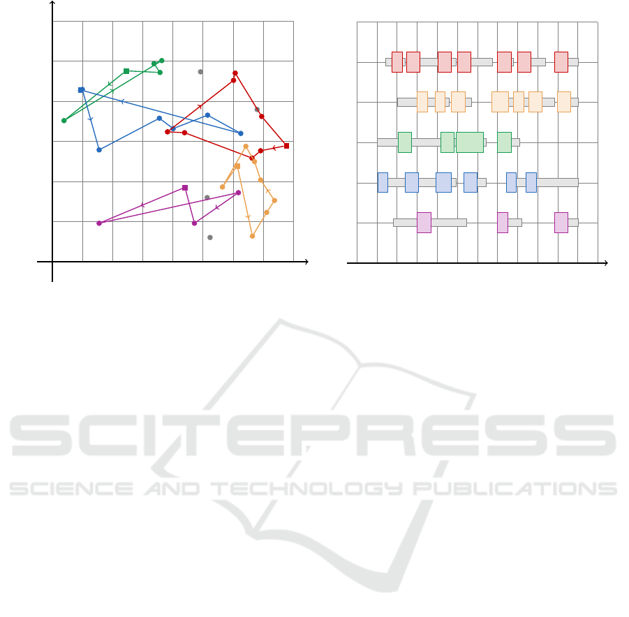
over a one-day horizon. Figure 1 displays the solu-

tion obtained with an optimization software. Each

employee is associated with a color (e.g. the red one

is related to the employee Ellen). The graph on the

left represents the employees’ routes: colored dots

are tasks performed by employees and gray ones non-

performed tasks, while squares correspond to employ-

ees’ starting locations. The Gantt chart on the right

depicts the employees’ schedules: higher and colored

rectangles represent tasks; smaller and gray ones rep-

resent employees’ traveling times to go from one task

to another; for both groups, the width of a rectangle

matches the duration of what it represents.

Facing this solution, an end-user may be surprised

by the fact that the task 15 is not performed by Ellen

(El in Figure 1) while it is not far from her route.

Then, the end-user may wish to get an explanation

to clear up the situation.

Lerouge, M., Gicquel, C., Mousseau, V. and Ouerdane, W.

Counterfactual Explanations for Workforce Scheduling and Routing Problems.

DOI: 10.5220/0011639900003396

In Proceedings of the 12th International Conference on Operations Research and Enterprise Systems (ICORES 2023), pages 50-61

ISBN: 978-989-758-627-9; ISSN: 2184-4372

 2023 by SCITEPRESS – Science and Technology Publications, Lda. Under CC license (CC BY-NC-ND 4.0)

14.5 14.75 15.0 15.25 15.5 15.75 16.0 16.25

47.25

47.5

47.75

48.0

48.25

48.5

longitude

latitude

7AM

9AM 11AM 1PM 3PM 5PM

7PM

hour

30 3

16 25

13 18

4 22

Figure 1: Representation of a WSRP solution (Lerouge et al., 2022).

For optimization experts, answering such queries

for explanations requires a lot of time and effort. It

namely involves getting familiar with the instance

and the solution, investigating the data without being

overwhelmed by the high combinatorial aspect of the

problem and ﬁnding concise pieces of explanations

to provide to the end-user. However, providing these

explanations is necessary as it helps to preserve the

end-users’ trust in the system and their conﬁdence at

work by enhancing their understanding of the results.

Thus, developing techniques for automatically gener-

ating explanations in response to end-users questions

would improve both end-users’ and optimization ex-

perts’ situations.

Automatic generation of explanations in the con-

text of decision support tools falls within the ﬁeld

of eXplainable Artiﬁcial Intelligence (XAI) (Gunning

and Aha, 2019) and has been heavily studied by the

machine learning community over the past decade

(Barredo Arrieta et al., 2020). However, to our knowl-

edge, few works addressed this topic for decision sup-

port tools solving CO problems: see (Ludwig et al.,

2018;

Cyras et al., 2019; Korikov et al., 2021). More-

over, these works rely on strong assumptions about

the studied CO problem and the provided explana-

tions that limit their applicability to other CO prob-

lems, such as the WSRP.

A noticeable exception is the work of (Lerouge

et al., 2022). The authors propose to tackle this is-

sue in the context of the WSRP by focusing on ex-

planations provided in response to “why-not” ques-

tions, also known as contrastive questions, i.e. ques-

tions having the following form “why not that fact in-

stead of this one?” (Lipton, 1990). Essentially, the

proposed method is based on identifying and narrat-

ing conﬂicts between the instance data and “that other

fact” which the end-user was expecting to observe in

the solution. If we go back to our example, such a

contrastive question is e.g. “Why is Ellen not per-

forming task 15 in addition to her already-performed

tasks?”. In response to it, the authors design an expla-

nation that highlights conﬂicts, e.g. conﬂicts between

the availability time-windows of the tasks, which tells

why it is impossible to make Ellen performs the task

15 in her already-performed tasks without violating

some of the availability constraints.

From now on, let us name desideratum “that other

fact” which the end-user was expecting to observe

in the solution. The end-user may also raise ques-

tions differing from “why-not” questions, especially

questions like “how to make the desideratum possi-

ble?”. For instance, in the context of our illustrative

example, such a question may be “How to make Ellen

perform task 15 in addition to her already-performed

tasks?”. These “how-to” questions ask for counter-

factual explanations: given an input of a system and

its corresponding output, a counterfactual explanation

consists in presenting a change in the input that would

have resulted in a different output such as one sat-

isfying the end-user-speciﬁed desideratum. Counter-

factual explanations are attractive as they are easy to

comprehend and can be used to offer a path of re-

course to end-users receiving unfavorable decisions.

Moreover, it was argued by (Wachter et al., 2018) that

counterfactual explanations are well aligned with the

European Union’s General Data Protection Regula-

tion (GDPR) requirements (GDPR, 2016).

Recently, (Korikov et al., 2021) proposed a

Counterfactual Explanations for Workforce Scheduling and Routing Problems

method to compute counterfactual explanations for

CO problems by leveraging inverse optimization.

However, their method is restricted to a speciﬁc class

of CO problem which does not include the WSRP.

Besides, it assumes that at most one data element

(speciﬁcally a coefﬁcient in the objective function

which does not appear in any constraint) may be

changed to obtain the counterfactual explanation. In

our case, such an assumption does not hold, as all the

coefﬁcients involved in the objective function also are

in the constraints. Therefore, their method cannot be

straightforwardly applied to our WSRP case.

Thus, in this paper, we propose a new mathemat-

ical programming-based approach to compute coun-

terfactual explanations for an end-user of a WSRP-

solving system. Given a solution of a WSRP instance

as well as end-user’s questions focusing on this solu-

tion and satisfying certain assumptions, this method

provides counterfactual explanations. Such explana-

tions emphasize the few changes that may be operated

on the instance data, which would be enough for ob-

taining outputs satisfying the end-user’s desiderata.

The remainder of this article is organized as fol-

lows. In Section 2, we clarify our WSRP use case by

detailing the content of an instance, introducing at the

same time various notations, and presenting an Inte-

ger Linear Program modeling this problem. In Sec-

tion 3, we describe our approach for generating coun-

terfactual explanations, which are then provided to the

end-user of a WSRP-solving system. Finally, conclu-

sions and perspectives are given in Section 4.

2 WORKFORCE SCHEDULING

AND ROUTING PROBLEM

As mentioned in Section 1, the Workforce Schedul-

ing and Routing Problem (WSRP) consists of assign-

ing tasks to mobile workforce members and creating

a pair of routes and schedules for these members. In

this section, we describe our WSRP use case, more

precisely the content of any instance and its corre-

sponding Integer Linear Programming (ILP) model.

In our use case, we consider a scheduling hori-

zon of one day i.e. 1440 minutes. An instance in-

volves a set of employees E = {1, ..., n} and a set

of tasks T = {1, . .., m}. Each employee i ∈ E has a

name, a starting location, which we call home for the

sake of simplicity, a skill level ske

∈ N and working

time-window [lbe

, ube

] ⊆ [0, 1440] ∩ N. Each task

j ∈ T has a speciﬁc location, a required skill level

skt

∈ N, a duration dt

∈ N and an availability time-

window [lbt

, ubt

] ⊆ [0, 1440] ∩ N. We assume that

hours in time-windows are expressed in minutes from

12:00AM (e.g. 8:00AM = 480).

For performing tasks, employees leave their

homes when they start their working day and return

there when they end it. In order to model these

two home events, we introduce, for each employee

i ∈ E , a departure index d

as well as a return in-

dex r

- where all the indices d

and r

for i ∈ E

are different from each other and different from the

indices of T = {1, ... , m}. We then extend the

set of tasks T with the set of departure indices and

the set of return indices to form a set of activities

A = T ∪ {d

, ..., d

} ∪ {r

, ..., r

}. Besides, for

each employee i ∈ E, we note A

= T ∪ {d

, r

} the

set of activities obtained by extending T with the de-

parture and return indices of i.

Finally, an instance also involves traveling times.

The time needed to travel between two activities

( j,k) ∈ A

is assumed to be independent of the em-

ployee and is noted tr

∈ N.

The instance data on which Figure 1 is based are

given in the Table 2 of the Appendix A.

In order to model the WSRP using Integer Linear

Programming (ILP), we introduce two sets of deci-

sion variables.

The ﬁrst one corresponds to spatial decisions. We

introduce, for i ∈ E and ( j,k) ∈ A

with j 6= k, a bi-

nary variable U

i jk

such that U

i jk

= 1 if employee i per-

forms activity j and then moves to activity k; U

i jk

= 0

otherwise. By assigning tasks to employees and spec-

ifying the order in which the tasks are performed,

these variables deﬁne the route of each employee.

The second set of variables corresponds to tem-

poral decisions. We introduce, for each j ∈ T , the

integer variable T

that sets the time at which j starts

to be performed by an employee if it is.

Based on the data of the instance and the decision

variables that we previously described, we model the

WSRP using ILP as presented in Model 1.

The bi-objective function (1) is maximized ac-

cording to a lexicographic order: the ﬁrst objective

equals the total working time, and the second to the

opposite of the total travel time.

Flow constraints (2) to (4) ensure that the em-

ployees start from their homes, go from tasks to oth-

ers without splitting into multiple directions, and end

their working day at home. Skill constraints (5) en-

sure that an employee i can be assigned to a task

j only if i has a skill level higher than the one re-

quired for performing j. Occurrence constraints (6)

ensure that a task j must occur at most once within all

employees’ routes. Availability constraints (7) to (8)

ensure that if a task j is performed by an employee

then j must be started and ended within its availabil-

ity time-window [lbt

, ubt

]. Work and sequencing

ICORES 2023 - 12th International Conference on Operations Research and Enterprise Systems

lex max



∑

i∈E

∑

j∈T

∑

k∈A

, k6=d

, j

i jk

, −

∑

i∈E

∑

j∈A

, j6=r

∑

k∈A

, k6=d

, j

i jk



(1)

s.t.

∑

k∈A

, k6=d

= 1 ∀ i ∈ E (2)

∑

j∈A

, j6=r

i jr

= 1 ∀ i ∈ E (3)

∑

j∈A

, j6=k,r

i jk

∑

∈A

, j

6=d

ik j

∀ i ∈ E , ∀ k ∈ T (4)

∑

k∈A

, k6=d

, j

i jk

≤ 1

{skt

≤ske

}

∀ i ∈ E , ∀ j ∈ T (5)

∑

i∈E

∑

k∈A

, k6=d

, j

i jk

≤ 1 ∀ j ∈ T (6)

∑

i∈E

∑

k∈A

, k6=d

, j

i jk

lbt

≤ T

∀ j ∈ T (7)

≤

∑

i∈E

∑

k∈A

, k6=d

, j

i jk

(ubt

− dt

) ∀ j ∈ T (8)

∑

i∈E

(lbe

+tr

) ≤ T

∀ k ∈ T (9)

+ dt

∑

i∈E

i jk

≤ T



1 −

∑

i∈E

i jk



ubt

∀ ( j,k) ∈ T

, j 6= k (10)

+ dt

≤

∑

i∈E

i jr

(ube

−tr

) +



1 −

∑

i∈E

i jr



ubt

∀ j ∈ T (11)

i jk

∈ {0, 1} ∀ i ∈ E , ∀ j ∈ A

\ {r

}, ∀ k ∈ A

\ {d

, j}

∈ N ∀ j ∈ T

Model 1: Bi-objective Integer Linear Program modeling our Workforce Scheduling and Routing Problem use case.

constraints (9) to (11) ensure that if an employee i

performs a task j then j must be started and ended

within the working time-window [lbe

, ube

] of i.

The solution represented in Figure 1 is given in

Table 3 of the Appendix B.

Now that our use case has been speciﬁed, we can

proceed to the generation of counterfactual explana-

tions, which is the focus of the next section.

3 GENERATING

COUNTER-FACTUAL

EXPLANATIONS

As mentioned in Section 1, this paper presents an

approach for generating counterfactual explanations

for an end-user who works with an optimization sys-

tem solving instances of Workforce Scheduling and

Routing Problem (WSRP). In this section, we de-

scribe how, by starting from the end-user’s questions

and moving to Integer Linear Programming (ILP), we

manage to produce such counterfactual explanations.

3.1 End-User’s Questions

In our approach, we consider that the end-user spec-

iﬁes a question to request an explanation. Moreover,

the question - explanation pairs are such that: i) They

relate only to a given solution S of a instance, noted

I . ii) The question starts with the interrogative form

“how-to” to explicitly ask for counterfactual explana-

tions. iii) The question mentions a desideratum i.e.

a fact which is not observed in S that the end-user

would like to have in S (e.g. seeing a task that is not

performed by an employee in S be now performed by

this employee). In addition, we assume that we can

always ﬁnd ways to transform the solutions so as to

satisfy the end-user’s desideratum (e.g. inserting the

non-performed task in the employee’s route).

Table 1 lists potential questions which satisfy the

assumptions mentioned above. More precisely, it lists

template texts that can be used to express questions.

Each template text is associated with an identifying

label and contains one or several symbols h.i indicat-

ing ﬁelds to be speciﬁed with data from the instance

I (e.g. an employee or a task).

For instance, the end-user’s question, mentioned

in Section 1, “How to make Ellen perform the task 15

in addition to her already-performed tasks?” can be

Counterfactual Explanations for Workforce Scheduling and Routing Problems

Table 1: Non-exhaustive list of template texts for end-user’s questions.

Labels Template texts for end-user’s questions

(Q1) “How to make hemployee i

∗

i perform htask j

∗

i just after hactivity k

∗

i?”

(Q2) “How to make hemployee i

∗

i perform htask j

∗

i between two consecutive activities of their route?”

(Q3) “How to make hemployee i

∗

i perform any non-performed task between two consecutive activities of their route?”

(Q4) “How to make any employee perform htask j

∗

i between two consecutive activities of their route?”

(Q5)

“How to make hemployee i

∗

i perform htask j

∗

i in addition to their already-performed tasks

(even if it means changing their order)?”

(Q6) “How to make hemployee i

∗

i perform htask j

∗

i in place of htask k

∗

i?”

(Q7) “How to make hemployee i

∗

i perform htask j

∗

i in place of any of their already-performed task?”

(Q8) “How to make hemployee i

∗

i perform any non-performed task in place of htask k

∗

i?”

(Q9) “How to make any employee perform htask j

∗

i in place of one of their already-performed tasks?”

(Q10)

“How to make hemployee i

∗

i perform htask j

∗

i instead of any of their already-performed tasks

(even if it means changing their order)?”

(Q11) “How to make hemployee i

∗

i perform htask j

∗

i, later in their route, just after htask k

∗

i?”

(Q12) “How to make hemployee i

∗

i perform htask j

∗

i, earlier in their route, just before htask k

∗

i?”

(Q13) “How to make hemployee i

∗

i perform htask j

∗

i later in their route?”

(Q14) “How to make hemployee i

∗

i perform htask j

∗

i earlier in their route?”

(Q15) “How to make hemployee i

∗

i perform htask j

∗

i at another position in their route?”

(Q16) “How to make hemployee i

∗

i perform their already-performed tasks in a different order?”

obtained by ﬁlling (Q5) template text with ﬁelds val-

ues “Ellen” and “15”. In order to invoke this question

again, in future examples, we note it q

Before moving to the next section, let us highlight

what can be seen as a limiting requirement of our ap-

proach: as a person who provides explanations, one

needs to enumerate the end-user’s questions be enu-

merated and deﬁne them as template texts. However,

such a requirement helps providing a clear and rigor-

ous framework to our approach, while reaching our

main goal, which is generating counterfactual expla-

nations in response to various end-user’s questions.

That is why we also consider this requirement to be

reasonable.

In the following subsections, we describe how we

process an end-user’s question like q

3.2 From Questions to ILP Modeling

In order to answer an end-user’s question with a

counterfactual explanation, we exploit ILP. More pre-

cisely, given a question template text listed in Table 1,

we build a new small-size ILP model upon Model

1. This model aims at ﬁnding how to change the

instance data to obtain a solution satisfying the end-

user’s desideratum while minimizing the number and

magnitude of these changes. To do so, this ILP in-

volves decision variables and constraints which artiﬁ-

cially alter the instance data.

Let us emphasize that the ILP model to be built

differs according to the template text of Table 1 used

to ask the question. Due to space limitation, we

choose to only describe the ILP model associated to a

question expressed thanks to (Q5) template text, like

. However, similar contents could be developed for

questions based on other template texts from Table 1.

3.2.1 Preliminaries

Before presenting the ILP model corresponding to

the question q, we need to introduce some notations,

make additional assumptions about (Q5) template

text and specify which parts of the instance I we plan

to alter for the counterfactual explanation.

The text of q refers to a speciﬁc employee i

∗

well as a speciﬁc task j

∗

(both mentioned by (Q5)

text ﬁelds h.i) and is relative to the solution S. We in-

troduce T

∗

= { j

, j

, ..., j

} ∪{ j

∗

} ⊆ T the subset

of tasks formed by the tasks performed by i

∗

in S plus

the task j

∗

. For instance, in the case of q

, i

∗

is Ellen,

∗

is the task 15 and T

∗

= {1,3, 7,8,15,17,26,30}.

For obvious reasons, the task j

∗

should not be per-

formed by the employee i

∗

in the solution S . For the

sake of simplicity, we assumed more generally that

∗

is not performed by any employee, otherwise we

would have to deal with the changes to apply to this

other employee’s route and schedule which is not of

major signiﬁcance. Besides, we also assumed i

∗

skilled enough for performing j

∗

otherwise we would

have to alter either the skill level of i

∗

or j

∗

which is

ICORES 2023 - 12th International Conference on Operations Research and Enterprise Systems

not really reasonable in practice.

About instance alterations, we need to choose

which data of I can be changed and by how much.

Such choices depend on the application context. In

some cases, it might be possible to extend the time

window of a task; sometimes, it might be inconceiv-

able. Ultimately, the end-user should be the one who

decides which data can be altered or not. To illus-

trate our approach, we propose in this paper to allow

changes of the availability time-window [lbt

, ubt

]

and duration dt

for all tasks j in T

∗

. At the end of

Subsection 3.2, we will discuss other possible alter-

ation choices and their impact the ILP modeling.

3.2.2 The ILP Model

We can now proceed to the description of Model 2,

i.e. the ILP model used for computing the counter-

factual explanation that answers q. Model 2 is based

on Model 1 but differs from it on various aspects, as

detailed in the following paragraphs.

An overall difference between the two models is

that Model 2 focuses on optimizing only the route and

schedule of a single employee, namely i

∗

, whereas

Model 1 deals with the routes and schedules of all the

employees of E . Such a restriction to i

∗

in Model 2

is possible as the question q focuses on an end-user’s

desideratum about S which only relates to i

∗

and the

subset of tasks T

∗

The main consequence of this restriction is that

not all the decision variables of Model 1 are involved

in Model 2: only the binary variables U

i jk

with i = i

∗

and the integer variables T

with j ∈ T

∗

are indeed

necessary for the Model 2. In other words, optimiz-

ing Model 2 can be seen as ﬁxing in Model 1 all the

binary variables U

i jk

with i 6= i

∗

as well as all the in-

teger variables T

with j ∈ T \ T

∗

to the values they

take in S and focusing the optimization over the set

of the remaining variables - plus other decision vari-

ables which will be described later in this subsection.

Due to this reduction of the set of decision variables,

a Model 2 solution does not provide directly a Model

1 solution i.e. a solution of the instance I . However,

in Subsection 3.3, we will see how build a Model 1

solution from S and a Model 2 solution.

Other consequences of this restriction to i

∗

are

that: there are no sums over E or constraints repeated

over E in Model 2; sums indexed over T in Model 1

are indexed over T

∗

in Model 2; constraints repeated

over T in Model 1 are repeated over T

∗

in Model 2;

etc. Besides, this restriction leads to a drastic decrease

in the size of Model 2 compared with Model 1, which

helps to solve Model 2 faster.

Decision Variables. New kinds of decision vari-

ables are involved in Model 2, in addition to the spa-

tial ones, U

∗

with ( j,k) ∈ A

∗

such that j 6= k, and

the temporal ones, T

for j ∈ T

∗

, both introduced in

Section 2.

• First, two new integer variables T

∗

and T

∗

are

brought into play. Like T

∗

, they are related to the

time at which the task j

∗

starts to be performed

(by i

∗

): T

∗

(resp. T

∗

) corresponds to the time

at which i

∗

can start to perform j

∗

while having

all the time constraints related to the activities per-

formed by i

∗

before (resp. after) j

∗

satisﬁed and

while respecting the lower (resp. upper) bound of

the availability window of j

∗

. By the way we in-

volve them in Model 2, these two variables allow

us to guarantee the feasibility of this model: ei-

ther T

∗

> T

∗

and it means that inserting j

∗

in the

route of i

∗

is impossible despite the potential alter-

ations of I , either T

∗

= T

∗

and it means that the

insertion is possible, since all the time constraints

of the activities performed by i

∗

before and after

∗

are satisﬁed.

• Second, several integer variables, so-called alter-

ing variables, are involved in Model 2 to arti-

ﬁcially alter some data of the instance I . For

j ∈ T

∗

, three integer variables ∆DT

, ∆LBT

and

∆UBT

are introduced allowing respectively to re-

duce the duration dt

of task j, to decrease the

lower bound lbt

of its time-window and to in-

crease its upper bound ubt

. In addition to these

altering variables, we introduce ∆T

max

, an integer

variable for measuring the greatest value taken by

any of the altering variables.

• Third, for j ∈ T

∗

, we associate to the altering vari-

ables ∆DT

, ∆LBT

and ∆UBT

, the binary vari-

ables XDT

, X LBT

and XUBT

, which whether

equal to 1 or 0 indicates whether or not their cor-

responding altering variable take positive value.

Objective Function. In Model 2, a multi-objective

function (1’) is minimized according to a lexico-

graphic order.

1. As having T

∗

= T

∗

means that the insertion of j

∗

in the route of i

∗

is possible, the ﬁrst objective aims

at tightening the gap between the two variables T

∗

and T

∗

by minimizing the difference T

∗

− T

∗

Note that the constraint (12.a) prevents the differ-

ence T

∗

− T

∗

from being negative.

2. The second objective minimizes the total reduc-

tion of tasks duration induced by altering variables

∆DT

for j ∈ T

∗

. Its purpose is to enable decreas-

ing the duration of the performed tasks only if ex-

tending the tasks’ time-windows, via ∆LBT

and

∆UBT

, is not enough for successfully inserting j

∗

Counterfactual Explanations for Workforce Scheduling and Routing Problems

lex min



∗

− T

∗

∑

j∈T

∗

∆DT

, ∆T

max

∑

j∈T

∗

XDT

+ X LBT

+ XUBT

∑

j∈A

∗

, j6=r

∗

∑

k∈A

∗

, k6=d

∗

, j

∗



)

s.t.

∑

k∈A

∗

, k6=d

∗

= 1 (2

)

∑

j∈A

∗

, j6=r

∗

= 1 (3

)

∑

j∈A

∗

, j6=k,r

∗

∑

∈A

∗

, j

6=d

∗

k j

∀ k ∈ T

∗

)

∑

k∈A

∗

, k6=d

∗

, j

∗

= 1 ∀ j ∈ T

∗

)

lbt

− ∆LBT

≤ T

∀ j ∈ T

∗

\ { j

∗

} (7

.a)

lbt

− ∆LBT

∗

≤ T

∗

.b)

≤ ubt

+ ∆UBT

− dt

+ ∆DT

∀ j ∈ T

∗

\ { j

∗

} (8

.a)

∗

≤ ubt

∗

+ ∆UBT

∗

− dt

∗

+ ∆DT

∗

.b)

lbe

∗

+tr

∗

≤ T

∀ k ∈ T

∗

\ { j

∗

} (9

.a)

lbe

∗

+tr

∗

≤ T

∗

.b)

+ dt

− ∆DT

∗

≤ T



1 −U

∗



ubt

∀ j 6= k ∈ T

∗

\ { j

∗

} (10

.a)

∗

+ dt

∗

− ∆DT

∗

≤ T



1 −U

∗



ubt

∗

∀ k ∈ T

∗

\ { j

∗

} (10

.b)

+ dt

− ∆DT

∗

j j

∗

j j

∗

≤ T

∗



1 −U

∗

j j

∗



ubt

∀ j ∈ T

∗

\ { j

∗

} (10

.c)

+ dt

− ∆DT

≤ U

∗

(ube

∗

−tr

∗

) +



1 −U

∗



ubt

∀ j ∈ T

∗

\ { j

∗

} (11

.a)

∗

+ dt

∗

− ∆DT

∗

≤ U

∗

(ube

∗

−tr

∗

) +



1 −U

∗



ubt

∗

(11

.b)

∗

− T

∗

≥ 0 (12.a)

∗

≤ T

∗

≤ T

∗

(12.b)

∆DT

≤ X DT

∀ j ∈ T

∗

(13.a)

∆LBT

≤ X LBT

max(lbt

− lbe

∗

, 0) ∀ j ∈ T

∗

(13.b)

∆U BT

≤ XUBT

max(ube

∗

− ubt

, 0) ∀ j ∈ T

∗

(13.c)

∆DT

, ∆LBT

, ∆UBT

≤ ∆T

max

∀ j ∈ T

∗

(14)

∗

∈ {0, 1} ∀ j ∈ A

∗

\ {r

∗

}, ∀ k ∈ A

∗

\ {d

∗

, j}

∈ N ∀ j ∈ T

∗

, T

∗

∈ N

XDT

, X LBT

, XUBT

∈ {0, 1} ∀ j ∈ T

∗

∆DT

, ∆LBT

, ∆UBT

∈ N ∀ j ∈ T

∗

∆T

max

∈ N

Model 2: Multi-objective program used for computing the explanation that answers a question based on (Q5) template text.

Such a preference for altering ﬁrst time-windows

and then duration is applied as decreasing tasks’

duration actually depreciates the solution since, by

Model 1, the primary objective is to maximize the

total tasks duration performed by the employees.

3. The purpose of the third objective which mini-

mizes ∆T

max

is to prevent alterations from being

too large, as much as possible.

4. The one of the fourth is to prevent them being too

numerous, as much as possible.

5. Lastly, the ﬁfth objective is linked to the second of

Model 1 as it minimizes the total traveling time.

Constraints. Most constraints of the Model 1 still

apply in the Model 2 but must be adapted. Flow con-

straints (2) to (4) correspond to constraints (2’) to (4’);

however (2’) to (4’) zoom on the employee i

∗

and the

subset T

∗

while (2) to (4) involve the whole sets E

and T . Occurrence constraint (5) coincide with con-

ICORES 2023 - 12th International Conference on Operations Research and Enterprise Systems

straint (5’) but in the latter, as we look for adding j

∗

among the tasks performed by i

∗

, all the tasks of T

∗

must be performed by i

∗

hence the use of = in (5’) in-

stead of ≤ in (5). No equivalent of the skill constraint

(6) appears in the Model 2 as i

∗

is supposed to have a

higher skill level than the ones of all the tasks of T

∗

(see our assumptions in Subsection 3.2.1). Availabil-

ity, working hours and sequencing constraints span-

ning labels from (7) to (11) in Model 1 are also in-

volved, with some changes, in Model 2 as labels span-

ning from (7’.a) to (11’.b). Each original constraint

of Model 1 (e.g. constraint (7)) is split into two or

three constraints in Model 2 (e.g. constraints (7’.a)

and (7’.b)) in order to separate the case of j

∗

, which

involves T

∗

and T

∗

, from the one of any other task

j in T

∗

, which involves T

In addition, new constraints are introduced in

Model 2. As mentioned earlier, constraint (12.a) pre-

vents the difference T

∗

− T

∗

from being negative.

Constraint (12.b) is simply used for controlling T

∗

value which is no longer involved in any constraint.

Constraints (13.a) to (13.c) ensure that the binary vari-

ables XDT

, XLBT

and XUBT

for j ∈ T

∗

play their

expected role, namely indicating whether or not their

corresponding altering variable take a positive value.

Besides, these constraints limit the value of the al-

tering variables ∆DT

, ∆LBT

and ∆U BT

for j ∈ T

∗

to some “reasonable bounds”: the duration dt

of a

task j can not be reduced by more than its own value;

there is no point in having the lower and upper bounds

of the availability time-window of task respectively

smaller and higher than the lower and upper bounds

of the working time-window of employee i

∗

. Fi-

nally, constraint (14) ensure that ∆T

max

measures as

expected the greatest value taken by any of the alter-

ing variables.

Discussion. Before ending this Subsection 3.2, let

us comeback to the discussion, started up in Subsec-

tion 3.2.1, about the way I can be altered, in particular

which data can be changed and up to what bounds.

It is clear that there are many ways to alter the data

of I . In this paper, we chose to locate the potential

alterations on task availability time-window and du-

ration data, to allow such alterations on all the tasks

of T

∗

and to limit such alterations to some “reason-

able bounds”. However, one could also choose, for

instance, to locate alterations on employee working

time-window data in addition to the ones on the task

data, to allow task alterations only for some selected

tasks of T

∗

, and to bound altering variables with ar-

bitrary smaller bounds than our “reasonable bounds”.

Still, such other choices could actually be taken

into account in Model 2 considering some adaptions.

One would have i) to introduce a pair of integer vari-

ables ∆LBE

∗

and ∆UBE

∗

, as well as their corre-

sponding binary variables XLBE

∗

and XUBE

∗

, for

altering the time-window of i

∗

; ii) to only consider

∆LBT

, ∆U BT

and ∆DT

for the selected tasks of T

∗

;

iii) to adapt the fourth objective in the multi-objective

function; iv) to adapt constraints (7’.a) to (11’.b) to in-

volve ∆LBE

∗

and ∆UBE

∗

as well as ∆LBT

, ∆UBT

and ∆DT

only for the selected tasks of T

∗

; v) replace

the “reasonable bounds” in constraints (13.a) to (13.c)

with arbitrarily chosen bounds; etc.

Thus, we can let the end-user - who is actually

the person who knows the best the application con-

text of the WSRP solved - choose the locations and

the bounds of the potential alterations to apply on the

data of I and still be able to deﬁne a Model 2 adapted

to such choices.

To conclude, this Subsection 3.2 was devoted to

describe how we move from the end-user’s question

q to an ILP model, namely Model 2. In the follow-

ing subsection, we present how we exploit an optimal

solution of Model 2 to produce a counterfactual ex-

planation.

3.3 From ILP Modeling to Explanations

As a continuation of Subsection 3.2, in this subsec-

tion, we keep focusing on a question q that relates to

a solution S of a WSRP instance I that is expressed

thanks to (Q5) template text. In addition, we assume

that we obtained an optimal solution of Model 2 that

is associated with q. Such a solution can be obtained

using any ILP solver on the Model 2. Note that solv-

ing Model 2 requires a reasonable computational ef-

fort thanks to the drastic reduction in the model size

that we obtained by restricting the model to the route

and schedule of i

∗

(c.f. Subsection 3.2.2).

As mentioned in Subsection 3.2.2, due to the re-

duction of the set of decision variables in Model 2 to

the U

i jk

such that i = i

∗

and the T

such that j ∈ T

∗

a Model 2 solution is not directly a solution of Model

1 i.e. a solution of I . However, given S and a Model

2 solution, we can build a new Model 1 solution as

follows. Let us note S

a solution of Model 2. By re-

placing in S the values of the decision variables which

are common to Model 1 and Model 2 with the values

that these variables take in S

, we can build a new so-

lution S

of the Model 1.

In particular, when S

is an optimal solution of

Model 2, we call the solution S

a neighboring solu-

tion of S induced by Model 2. Note that in most cases

is likely to be infeasible relatively to I as S

likely to have positive altering variables correspond-

ing to necessary alterations of I .

Similarly, we can deﬁne a notion of neighboring

Counterfactual Explanations for Workforce Scheduling and Routing Problems

instance of I induced by Model 2. Indeed, Model 2

contains not only decision variables which are shared

with Model 1 but also its own decision variables like

the altering ones. By changing the data of I according

to the values taken by these altering variables S

, we

can build a new WSRP instance I

. Again, when S

an optimal solution of Model 2, we call such instance

a neighboring instance of I induced by Model 2.

Note that in most cases I

6= I .

From now on, in addition to q, S and I already

introduced, let us consider S

an optimal solution of

Model 2 that is related to q, S

a neighboring solu-

tion of S induced by Model 2 and I

a neighboring

instance of I induced by Model 2.

We identify three possible cases based on the val-

ues taken by decision variables in the optimal solution

of Model 2.

Case 1: T

∗

− T

∗

= 0 and ∆T

max

> 0.

Case 2: T

∗

− T

∗

= 0 and ∆T

max

= 0.

Case 3: T

∗

− T

∗

> 0.

Case 1 corresponds to the case where by resorting to

some alterations of the data of I , it is possible to ob-

tain the end-user’s desideratum (i.e. it is possible to

make employee i

∗

perform the task j

∗

in addition to

their already-perform tasks, knowing that q is a ques-

tion based on (Q5) template text). In other words,

the neighboring solution S

is feasible relatively to the

neighboring instance I

and I

6= I .

The counterfactual explanation for Case 1 can be

expressed as follows: “By happlying the instance al-

terations associated with all the non-zero altering

variables causing I 6= I

i, hthe desideratumi would

be possible; in this case, the solution would be

hdescription of S

i”

Case 1 is actually the case encountered for an-

swering q

, our illustrative example question intro-

duced in Section 1. Indeed, the counterfactual expla-

nation is “By changing the opening time of task 17,

from its value 12:30PM in the current input data, to

12:29PM instead, making Ellen perform the task 15

in addition to her already-performed tasks would be

possible; in this case, the solution would be the one

obtained by changing Ellen’s sequence of performed

tasks to [30, 7, 8, 1, 17, 15, 26, 3].”

Case 2 corresponds to the case where it is possible

to obtain the end-user’s desideratum without even re-

sorting to any alterations of the data of I . In other

words, the neighboring solution S

is feasible rela-

tively to the original instance I (and I

= I ).

In practice, knowing that q is a question based on

(Q5) template text, such case is actually expected not

to occurred so often. Indeed, as q asks for adding a

non-performed task j

∗

to the already-performed tasks

of an employee i

∗

, if the transformed solution is fea-

sible then it would necessarily be better than S . How-

ever, if S has been obtained thanks to an optimization

system applied on I, S should be a good solution, pos-

sibly even an optimal one, which can not be improved

by local transformations. Therefore, transforming S

to satisfy the end-user’s desideratum should certainly

result in an infeasible solution.

The counterfactual explanation for Case 2 can be

expressed as follows: “Without altering any data of

the current instance, hthe desideratumi is possible;

the solution is hdescription of S

i.”

Case 3 corresponds to the case where it is not pos-

sible to obtain the end-user’s desideratum despite the

possibility of altering the date of I .

Facing this situation, we could have provided a

simple explanation text telling that it is not possible

to obtain the desideratum despite all the possible al-

terations of the data of I . However, thanks to the

decision variables T

∗

and T

∗

, which guarantee the

feasibility of Model 2 (c.f. Subsection 3.2), even if

the insertion of j

∗

in the route of i

∗

is not possible

despite the alterations of I , we can still build a neigh-

boring solution S

and a neighboring instance I

. In

such case, S

is admittedly infeasible relatively to I

but S

can be interpreted as the solution satisfying the

desideratum that is the closest to be feasible relatively

to I . We can then use this information to enrich the

explanation text provided to the end-user.

The counterfactual explanation for Case 3 can be

expressed as follows: “Despite all the possible alter-

ations of the current instance data, hthe desideratumi

is not possible. The best that could be done con-

sists in happlying the instance alterations associated

with all the non-zero altering variables causing I 6=

i; in this case, the best solution satisfying hthe

desideratumi is the solution hdescription of S

i which

is not valid though.”

To conclude, in this Subsection 3.3, we presented

how the result of Model 2 can be used to build

a counterfactual explanation answering to the end-

user’s question q by identifying three cases and adapt-

ing the explanation text in consequences.

4 CONCLUSION

In this paper, we proposed a new approach, based

on mathematical programming, to compute counter-

factual explanations for an end-user of an optimiza-

tion system solving the Workforce Scheduling and

Routing Problem (WSRP), that we modeled as a bi-

objective Integer Linear Programming (ILP) model.

We considered that, facing a solution S of a WSRP

instance I that was provided by an optimization sys-

ICORES 2023 - 12th International Conference on Operations Research and Enterprise Systems

tem, the end-user requests explanations by expressing

questions which satisfy certain assumptions. Among

others, these questions must be about S and focus on

an end-user’s recourse about it. We provided a non-

exhaustive list of template texts for formulating such

questions.

Given an end-user’s question q, we associated

q with a multi-objective ILP model. This model

involves altering variables which enable precise

changes in the instance I data. The purpose of this

ILP model is to look for the changes to operate on

I for obtaining a new solution S

satisfying the end-

user’s desideratum.

In terms of future works, there are various re-

search topics that we would like to explore. Among

others, one of them is to evaluate our approach in

terms of beneﬁts brought by our explanations to the

end-user. A second is to transpose our approach to

other Combinatorial Optimization problems than the

WSRP to investigate its genericity.

ACKNOWLEDGEMENTS

This work has been supported by the project PSPC

AIDA: 2019- PSPC-09 funded by BPI-France. We

thank Daniel Godard, Filippo Focacci and Desir

Rigonat from DecisionBrain for their time and their

helpful feedback throughout this work.

REFERENCES

Barredo Arrieta, A., D

ıaz-Rodr

ıguez, N., Del Ser, J., Ben-

netot, A., Tabik, S., Barbado, A., Garcia, S., Gil-

Lopez, S., Molina, D., Benjamins, R., Chatila, R.,

and Herrera, F. (2020). Explainable Artiﬁcial Intel-

ligence (XAI): Concepts, taxonomies, opportunities

and challenges toward responsible AI. Information fu-

sion, 58:82–115.

Castillo-Salazar, J. A., Landa-Silva, D., and Qu, R. (2016).

Workforce Scheduling and Routing Problems: litera-

ture survey and computational study. Annals of Oper-

ations Research, 239:39 – 67.

Chen, X., Thomas, B. W., and Hewitt, M. (2016). The

Technician Routing Problem with experience-based

service times. Omega, 61:49–61.

Cyras, K., Letsios, D., Misener, R., and Toni, F. (2019). Ar-

gumentation for Explainable Scheduling. In Proceed-

ings of the thirty-third Association for the Advance-

ment of Artiﬁcial Intelligence Conference on Artiﬁcial

Intelligence, pages 2752 – 2759. AAAI Press.

DecisionBrain (2022). Decisionbrain s.a.s. https://decision

brain.com/. Accessed 2022-10-10.

Euchi, J., Masmoudi, M., and Siarry, P. (2022). Home

health care routing and scheduling problems: a litera-

ture review. 4OR, pages 1–39.

GDPR (2016). Regulation (EU) 2016/679 of the European

Parliament and of the Council of 27 April 2016 on the

protection of natural persons with regard to the pro-

cessing of personal data and on the free movement of

such data, and repealing Directive 95/46/EC (General

Data Protection Regulation).

Gunning, D. and Aha, D. (2019). DARPA’s Explainable

Artiﬁcial Intelligence (XAI) program. AI Magazine,

40:44–58.

Korikov, A., Shleyfman, A., and Beck, C. (2021). Counter-

factual explanations for optimization-based decisions

in the context of the GDPR. In Proceedings of the

thirtieth International Joint Conference on Artiﬁcial

Intelligence, pages 4097 – 4103. IJCAI Organization.

Lerouge, M., Gicquel, C., Mousseau, V., and Ouerdane,

W. (2022). Explaining solutions stemming from op-

timization systems solving the Workforce Scheduling

and Routing Problem to their end-users. Working pa-

per https://hal.archives-ouvertes.fr/hal-03795653.

Lipton, P. (1990). Contrastive explanation. Royal Institute

of Philosophy Supplement, 27:247–266.

Ludwig, J., Kalton, A., and Stottler, R. (2018). Explain-

ing complex scheduling decisions. In Intelligent User

Interfaces Workshops.

Wachter, S., Mittelstadt, B., and Russell, C. (2018). Coun-

terfactual explanations without opening the black box:

Automated decisions and the GDPR. Harvard Journal

of Law & Technology, 31.

Counterfactual Explanations for Workforce Scheduling and Routing Problems

APPENDIX

Appendix A. Instance

Table 2: An example of WSRP instance. The ﬁrst table describes the data about the set of employees E . Each employee

i ∈ E is characterized by a skill level ske

, a departure and return location, and a time-window [lbe

, ube

]. The second table

describes the data about the tasks. Each task j is described by a skill level skt

, a location, a duration dt

and a time-window

[lbt

, ubt

]. It is assumed that all the employees have the same traveling speed of 50km/h. Considering that the earth radius

is 6731km, the traveling time, in minutes, between two locations (lat

, long

) and (lat

, long

) can be computed as follows:

6731 × arccos(sin(lat

) × sin(lat

) + cos(lat

) × cos(lat

) × cos(long

− long

))/50 × 60. (Lerouge et al., 2022)

Employee Name Skill level Location Time-window

i ske

[lbe

, ube

]

in E in N

as (lat., long.) in deg. as time range as integer range

1 Ellen 2 (47.773, 16.193) [8:00AM, 6:00PM] [480, 1080]

2 Alex 3 (47.598, 15.785) [9:00AM, 6:00PM] [540, 1080]

3 Adam 2 (48.188, 14.862) [8:00AM, 6:00PM] [480, 1080]

4 Fabian 1 (48.069, 14.485) [8:00AM, 6:00PM] [480, 1080]

5 Carlotta 1 (47.463, 15.351) [8:00AM, 6:00PM] [480, 1080]

Task Skill level Location Duration Time-window

j skt

[lbt

, ubt

]

in T in N

as (lat., long.) in deg. in min. as time range as integer range

1 1 (48.129, 15.754) 40 [8:00AM, 6:00PM] [480, 1080]

2 1 (47.240, 15.430) 40 [2:00PM, 6:00PM] [840, 1080]

3 1 (47.803, 15.348) 40 [11:00AM, 6:00PM] [660, 1080]

4 1 (47.913, 15.539) 30 [2:00PM, 6:00PM] [840, 1080]

5 1 (47.240, 14.639) 40 [8:00AM, 12:00PM] [480, 720]

6 3 (47.719, 15.856) 40 [8:00AM, 6:00PM] [480, 1080]

7 2 (47.691, 15.979) 30 [8:45AM, 12:00PM] [525, 720]

8 1 (47.904, 15.988) 40 [8:00AM, 6:00PM] [480, 1080]

9 1 (48.252, 15.159) 40 [9:00AM, 12:00PM] [540, 720]

10 2 (48.233, 15.094) 80 [9:00AM, 6:00PM] [540, 1080]

11 2 (47.879, 14.348) 40 [8:00AM, 6:00PM] [480, 1080]

12 2 (47.151, 15.559) 40 [8:00AM, 6:00PM] [480, 1080]

13 1 (48.073, 14.500) 30 [8:00AM, 6:00PM] [480, 1080]

14 1 (47.509, 15.979) 50 [8:00AM, 6:00PM] [480, 1080]

15 2 (48.182, 15.480) 25 [8:00AM, 2:00PM] [480, 840]

16 1 (47.307, 16.030) 30 [8:00AM, 6:00PM] [480, 1080]

17 1 (48.174, 15.768) 40 [12:30PM, 4:00PM] [750, 960]

18 1 (47.696, 14.639) 40 [8:00AM, 6:00PM] [480, 1080]

19 2 (47.466, 15.662) 40 [8:00AM, 6:00PM] [480, 1080]

20 2 (47.624, 15.928) 30 [8:00AM, 6:00PM] [480, 1080]

21 1 (47.893, 15.139) 45 [8:00AM, 6:00PM] [480, 1080]

22 1 (47.799, 15.814) 30 [3:00PM, 6:00PM] [900, 1080]

23 1 (47.430, 15.794) 30 [10:00AM, 3:00PM] [600, 900]

24 2 (48.178, 15.144) 40 [2:00PM, 3:00PM] [840, 900]

25 1 (47.382, 16.094) 40 [8:00AM, 1:00PM] [480, 780]

26 2 (47.809, 15.206) 40 [12:00PM, 6:00PM] [720, 1080]

27 2 (47.948, 15.950) 50 [8:00AM, 3:00PM] [480, 900]

28 3 (47.160, 15.991) 30 [8:00AM, 6:00PM] [480, 1080]

29 1 (47.829, 15.253) 40 [8:00AM, 1:00PM] [480, 780]

30 1 (47.646, 15.907) 40 [8:00AM, 12:00PM] [480, 720]

31 2 (47.399, 15.535) 40 [8:00AM, 4:00PM] [480, 960]

ICORES 2023 - 12th International Conference on Operations Research and Enterprise Systems

Appendix B. Solution

Table 3: An example of solution of the WSRP instance described in Table 2. This solution also represented in Figure 1. The

ﬁrst table gives the values of the binary decision variables U

i jk

and the second table gives the values of the integer decision

variables T

. (Lerouge et al., 2022)

Employee Binary decision variables

i U

i, j,k

1,d

= U

1,7,30

= U

1,30,3

= U

1,3,26

= U

1,26,1

= U

1,1,17

= U

1,17,8

= U

1,8,r

= 1

1, j,k

= 0 for all other couples of activities (j,k)

2,d

,28

= U

2,28,16

= U

2,16,25

= U

2,25,14

= U

2,14,20

= U

2,20,6

= U

2,6,19

= U

2,19,r

= 1

2, j,k

= 0 for all other couples of activities (j,k)

3,d

,11

= U

3,11,9

= U

3,9,10

= U

3,10,24

= U

3,24,r

= 1

3, j,k

= 0 for all other couples of activities (j,k)

4,d

,13

= U

4,13,18

= U

4,18,21

= U

4,21,29

= U

4,29,14

= U

4,14,22

= U

4,22,r

= 1

4, j,k

= 0 for all other couples of activities (j,k)

5,d

= U

5,5,23

= U

5,23,2

= U

5,2,r

= 1

5, j,k

= 0 for all other couples of activities (j,k)

Task Integer decision variables

j T

1 840

2 1009

3 662

4 866

5 600

6 933

7 525

8 1009

9 670

10 717

11 542

12 0

13 482

14 822

15 0

16 653

Task Integer decision variables

j T

17 900

18 564

19 1019

20 888

21 656

22 925

23 840

24 840

25 702

26 720

27 0

28 600

29 738

30 567

31 0

blank

Counterfactual Explanations for Workforce Scheduling and Routing Problems