Dealing with Overﬁtting in the Context of Liveness Detection Using

FeatherNets with RGB Images

Miguel Le

1 a

and Nuno Gonc¸alves

1, 2 b

Institute of Systems and Robotics, University of Coimbra, Portugal

Portuguese Mint and Ofﬁcial Printing Ofﬁce (Imprensa Nacional-Casa da Moeda SA), Portugal

Keywords:

FeatherNets, Overﬁtting, Bonaﬁde, Spoof, Dataset.

Abstract:

With the increased use of machine learning for liveness detection solutions comes some shortcomings like

overﬁtting, where the model adapts perfectly to the training set, becoming unusable when used with the testing

set, defeating the purpose of machine learning. This paper proposes how to approach overﬁtting without

altering the model used by focusing on the input and output information of the model. The input approach

focuses on the information obtained from the different modalities present in the datasets used, as well as how

varied the information of these datasets is, not only in number of spoof types but as the ambient conditions

when the videos were captured. The output approaches were focused on both the loss function, which has

an effect on the actual ”learning”, used on the model which is calculated from the model’s output and is

then propagated backwards, and the interpretation of said output to deﬁne what predictions are considered

as bonaﬁde or spoof. Throughout this work, we were able to reduce the overﬁtting effect with a difference

between the best epoch and the average of the last ﬁfty epochs from 36.57% to 3.63%.

1 INTRODUCTION

With the rise of facial recognition technology in day-

to-day applications, such as mobile payments, comes

a concern for the security of these systems. To coun-

teract these security vulnerabilities, which present

themselves as Presentation Attacks (PA), the develop-

ment of Presentation Attack Detection (PAD) or live-

ness detection has become a requisite of modern facial

recognition systems.

Currently, most methods are based in machine

learning, more speciﬁcally Convolutional Neural Net-

works (CNN) or a variation of these, which are

trained by feeding them large quantities of informa-

tion extracted from datasets with images from various

modalities, be it colour images (RGB, HSV, YCbCr),

depth maps or even infrared images.

A well known issue in learning systems is overﬁt-

ting, where the model fully adapts to a speciﬁc portion

of the data presented turning useless for the informa-

tion as a whole. The overﬁtting problem in liveness

detection can then be attributed to certain factors like

the binary nature of the problem itself: ”bonaﬁde or

spoof?”.

https://orcid.org/0000-0002-6842-8009

https://orcid.org/0000-0002-1854-049X

To mitigate the overﬁtting issue, there are several

approaches that try to optimize the model or aid the

typically colour images with extra information to con-

ﬁrm certain factors associated with the different types

of attacks present in the datasets.

This requires considerable additional work in as-

sociating the supervising information to the already

present dataset or in optimizing the models to deal

with a speciﬁc issue which may require compromises

that result in other shortcomings. Attempting to re-

solve these issues, this paper explores different ap-

proaches in mitigating overﬁtting without adapting

the model used or resorting to common techniques

like early stopping.

The objective is to reduce the overall requirements

of liveness detection solutions, be it in computational

requirements, monetary cost or information require-

ments in order to apply these solutions to the systems

that would most beneﬁt from them.

The initial baseline result of 99.32% accuracy, ob-

tained with depth images, gave little room for im-

provement so a new baseline using RGB images,

which constitutes a more realistic scenario for com-

mon systems resorting only to RGB cameras without

depth information, was obtained. These results are

not only less successful with an accuracy of 89.75% ,

but display overﬁtting with the average of the model’s

Leão, M. and Gonçalves, N.

Dealing with Overﬁtting in the Context of Liveness Detection Using FeatherNets with RGB Images.

DOI: 10.5220/0011639600003411

In Proceedings of the 12th International Conference on Pattern Recognition Applications and Methods (ICPRAM 2023), pages 62-73

ISBN: 978-989-758-626-2; ISSN: 2184-4313

 2023 by SCITEPRESS – Science and Technology Publications, Lda. Under CC license (CC BY-NC-ND 4.0)

last 50 accuracy results being 53.18%, a drop of

36.57% in accuracy which can be attributed to over-

ﬁtting issues. Through this work, while unable to im-

prove the result from the best epoch, the developed

approaches were able to remove or at least heavily

lower the overﬁtting effect, with the top accuracy of

89.37% then achieving an average of the ﬁnal 50 re-

sults equal to 85.75%.

2 LITERATURE REVIEW

Since the question of liveness detection can be put

bluntly as ”bonaﬁde or spoof” the ﬁrst machine

learning solutions employ binary cross-entropy loss

as the sole learning supervision for the network (Xu

et al., 2015; Menotti et al., 2015; Yang et al., 2014).

However due to its simplicity, the models are prone to

overﬁtting since they can easily focus their learning

in arbitrary features, not relevant to the liveness de-

tection problem. While the use of different loss func-

tions has been employed (Hao et al., 2019; Xu et al.,

2020) by interpreting the issue in other ways, another

solution was to aid the loss function using pixel-wise

supervision.

Pixel-wise supervision can be made by using pre-

vious knowledge of liveness detection, and applying

it to the model. For example, the use of pseudo depth

maps (Atoum et al., 2017; Yu et al., 2020) based on

the knowledge that, two dimensional attacks (print

and replay) will display a ”ﬂat” depth map can be used

to aid the model. By the same logic, binary mask la-

bels (Sun et al., 2020; Liu et al., 2019) or reﬂection

maps (Kim et al., 2019) have been used.

The previously mentioned approaches are all

based on colour inputs (RGB, YCbCr or HSV) and

it is the modality most commonly used. However,

thanks to the development in sensors, it is possible

to retrieve datasets using other modalities like depth,

infra-red or thermal images. The models can then use

a singular type of modality, or use the information

available from several modalities all at once.

One such work is FeatherNets developed by

Zhang et al. (Zhang et al., 2019a) in the interest of

adapting the current deep learning approaches to live-

ness detection, which are usually very heavy in both

computation requirements and data storage, to use in

mobile or embedded devices which are incapable of

meeting these requirements. To solve this problem,

they propose a network ”as light as a feather” that

using depth information is able to achieve ACER of

0.00168, with only 0.35 million parameters and 83

million ﬂops down from the baseline using ResNet18

(He et al., 2016) with an ACER of 0.05 with 11.18

million parameters and 1800 million ﬂops. This net-

work was chosen since its lightweight nature is in line

with the overall objective of our work.

Datasets are an essential part of any machine learn-

ing development, varying in data type, size and qual-

ity among other attributes and variables. While fa-

cial recognition/detection has been in development

since the 1960’s (Wayman, 2007) and as such has

accumulated a large number of datasets, the interest

in liveness detection only began in the 2010’s (Yu

et al., 2021). In this short time span, various datasets

have been developed by researchers and the industry,

steadily increasing the number of individuals present,

the number of images/videos, the quality and image

modalities, and perhaps of most interest to this pa-

per the number of different attacks present. From the

different choices of datasets present, which Yu et al.

(Yu et al., 2021) give a good overview of the publicly

available ones, two were chosen for this work:

CASIA-SURF, developed by Zhang et al. (Zhang

et al., 2019b), which presents a larger dataset than

most with 21,000 videos of 1,000 individuals cap-

tured with an Intel Real Sense 3000 camera providing

not only RGB images but also depth and infrared im-

ages. The information is neatly distributed with one

bonaﬁde video to six spoof videos of each individ-

ual in each of the modalities provided by the camera.

Where the dataset might be considered lacking is in

the number of different attacks, the six spoof videos

are all of print attacks. The print attacks were diversi-

ﬁed by how the print was placed over the individuals

face: either ﬂat or pressed curved, and also the fea-

tures of the print that were cut off: ﬁrst removing the

eyes, then the nose and ﬁnally the mouth. The con-

ditions in which the videos were captured in a ﬁxed

setup where the individual stands in front of a green

screen which displays various backgrounds without

speciﬁed changes to the lighting, the individuals were

then requested to tilt their heads, move closer and fur-

ther away from the camera and move up and down.

WMCA, developed by George et al. (George et al.,

2020), being quite smaller than the previous dataset

with 1,679 videos of 72 individuals, which are divided

in 347 bonaﬁde cases and 1,332 spoofs. This dataset

was constructed with the same camera as CASIA-

SURF having the same modalities, yet they added a

Seek Thermal Compact PRO to capture thermal im-

agery of the individuals. Despite the lower num-

ber of videos, WMCA has the advantage of having

a larger variety of attacks than CASIA-SURF adding

to the print attacks, video replays, glasses, fake heads

(mannequins), rigid masks, ﬂexible masks and pa-

per masks. These videos were captured with the in-

dividual on a ﬁxed position through seven different

Dealing with Overﬁtting in the Context of Liveness Detection Using FeatherNets with RGB Images

sessions, in these sessions both the background and

lighting varying, through uniform and complex back-

grounds and through natural light, ceiling lighting and

LED lighting.

In the context of deep learning, a loss function

is what evaluates how successfully the model is per-

forming: the lower the losses, the higher the success.

Janocha and Czarnecki state that most of deep learn-

ing models use binary cross entropy loss also known

as log loss (Janocha and Czarnecki, 2017). This ap-

plies well to liveness detection, considering that the

problem is at its root a simple yes or no question:

”Is this face bonaﬁde or not?”. However, due to the

simplicity of the loss function, these models can eas-

ily learn arbitrary patterns that deviate from the initial

question of bonaﬁde vs. spoof.

There have been several approaches attempting to

solve the shortcomings of binary cross entropy loss

by expanding on the problem like focal loss used in

(Lin et al., 2020), developed while attempting to solve

the issues present in a scenario of object detection

where there is a very large imbalance between the

foreground and background classes. It is built upon

the basic cross-entropy loss, adding a simple weight

balancing parameter to address class imbalance in the

dataset, and the focusing parameter in order to down-

weight the impact of the decisions made in easy ex-

amples i.e. the more classiﬁed categories.

3 APPROACH

For the most part, the work conducted for this pa-

per follows the methods presented by the authors of

FeatherNets, adding the use of the WMCA dataset

and resorting to the use of colour (RGB) information

instead of the original use of depth information. There

is however need to point out details of the approach

used and for the interpretation of the results.

The two key details on the use of both the net-

work and datasets used are the exclusion of the Multi-

Modal Fusion Strategy presented by Zhang et al.

(Zhang et al., 2019a), since the interest is only on the

colour modality, and the use of the free version of the

WMCA dataset. From the values presented in the lit-

erature review, the free version removes four spoof

types and from the remaining categories removes a

certain number of examples. While the distribution

of the WMCA dataset was made by dividing the in-

formation in roughly thirds and then distributing it

accordingly between the three sets (training, valida-

tion and testing) while making sure that each set had

representations not present on the other sets. The dis-

tribution chosen for these parts was a 60%/20%/20%

random pick from the images in table 1, ending in the

values presented by table 2.

Table 1: Distribution of presentations in the WMCA

dataset’s free version. The free version removes 4 types of

attacks and some examples from the categories that remain.

Category Number of Presentations

Bonaﬁde 205

Print Attack 193

Replay Attack 169

Flexible Mask 283

Total 850

Table 2: Statistical information of the WMCA dataset’s free

version and personal distribution between its training, test-

ing and validation sets. The distribution is made between

training set (Train.), validation set (Val.) and testing set

(Test.).

Train. Val. Test. Total

# Spoofs 387 129 129 645

# Bonaﬁde 123 41 41 205

# Videos 510 170 170 850

# Frames 25,500 8,500 8,500 42,500

3.1 Architecture

FeatherNets’ structure is based on a main block, a

down sampling block and then a streaming module

that substitutes the fully connected layer as to reduce

overﬁtting. The main block is based on the ”Mo-

bileNet v2” model proposed by Sandler et al. (San-

dler et al., 2018) which employs the use of depth wise

convolution as well as inverted Rectiﬁed Linear Unit

(ReLU) blocks to improve the computation require-

ments associated with the computer vision tasks.

The main block is then followed by one of two

down sampling blocks, creating the distinction be-

tween FeatherNetA and FeatherNetB. FeatherNetA’s

downsampler is the simpler of the two having a sin-

gular branch of the depth wise convolution/inverted

ReLU combination while increasing the stride of the

convolution to 2 thus reducing the dimensions of the

input to 12.5% of the original size. FeatherNetB’s

downsampler has also a ﬁrst branch equal to Feather-

NetA but adds a parallel secondary branch with aver-

age pooling to better learn more diverse features.

Both models are then followed by their proposed

streaming module that, by replacing the fully con-

nected layer, reduces the overﬁtting effect and use fo-

cal loss for their loss function, as seen in equation 1.

FocalLoss = −α

(1 − p

)

log(p

) (1)

where p

and α

are the estimated probability and

weighting factor to address class imbalance of any

ICPRAM 2023 - 12th International Conference on Pattern Recognition Applications and Methods

determined class, respectively and γ is the weighing

factor that regulates how much importance is given to

the ”harder” predictions over the ”easier” ones. For

further details on these topics, a reading of the origi-

nal articles (Zhang et al., 2019a) and (Lin et al., 2020)

is recommended.

3.2 Evaluation Metrics

In order to measure the success of any proposed

method in liveness detection, there is a number of

metrics that can be taken from the result’s confusion

matrix. In binary cases like the basic approach to live-

ness detection, one can immediately take the values

from the confusion matrix to obtain the true positive

(TP), false positive (FP), true negative (TN) and false

negative (FN) values, with which the following met-

rics can be calculated (Chingovska et al., 2014):

• Accuracy: The percentage of correct predictions

on the dataset;

Accuracy =

T P + T N

T P + FN + T N + FP

(2)

• Recall: Also known as True Positive Rate (TPR)

is the percentage of true values predicted as such;

Recall =

T P

T P + FN

(3)

• Speciﬁcity: Also known as True Negative Rate

(TNR) is the percentage of false values predicted

as such;

Speci f icity =

T N

T N + FP

(4)

• Precision: The percentage of correctly predicted

true cases among all predicted true cases;

Precision =

T P

T P + FP

(5)

• False Acceptance Rate: The percentage of false

cases that are wrongly accepted as true cases;

FAR =

FP + T N

= 1 − Speci f icity (6)

• False Rejection Rate: The percentage of true

cases that are wrongly mistaken for false cases;

FRR =

FN + T P

= 1 − Recall (7)

• Half Total Error Rate: The average of the previous

two metrics;

HT ER =

FAR + FRR

(8)

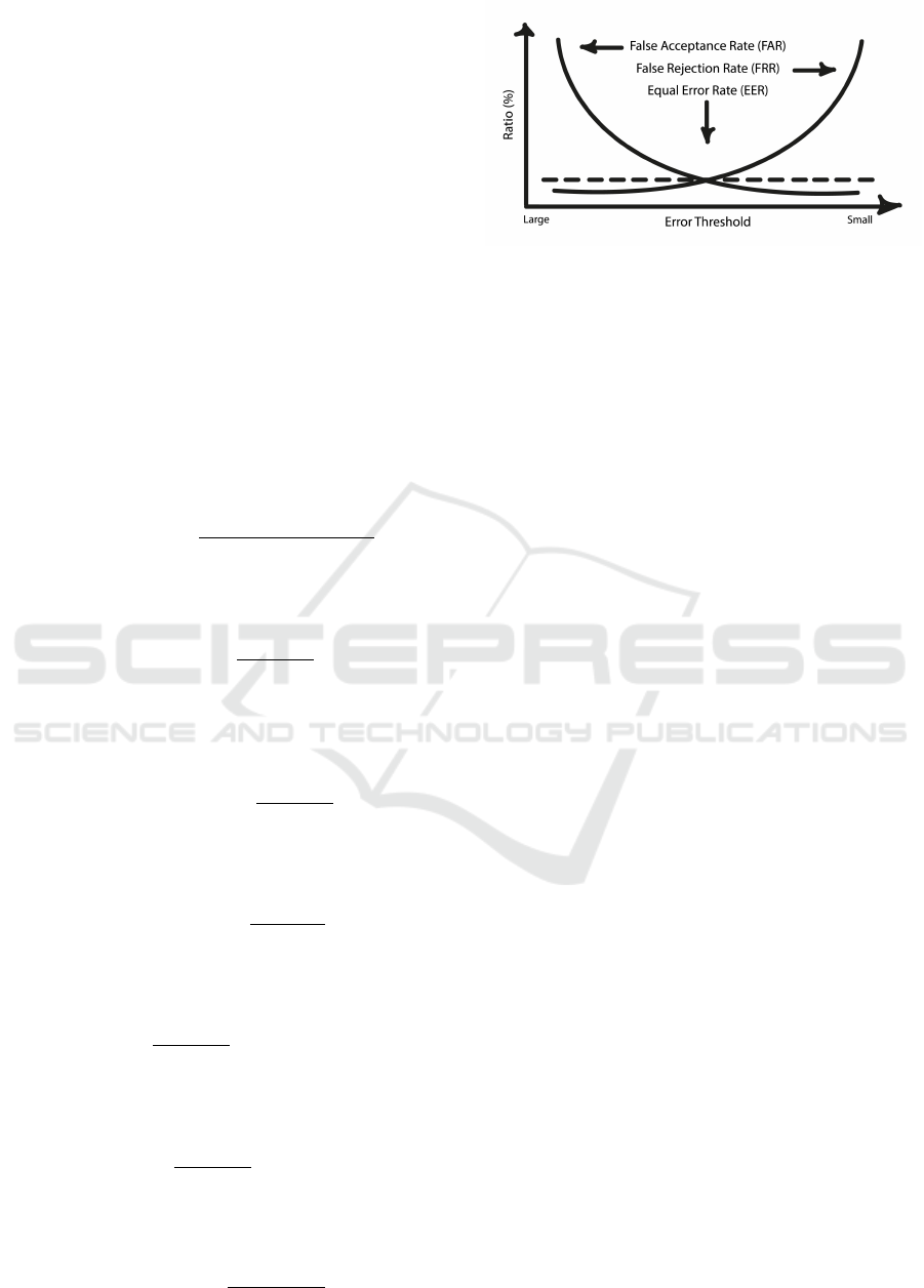
Figure 1: Relation between EER, FRR and FAR.

• Equal Error Rate: EER is the HTER when FAR

and FRR are equal;

Recently the terms Attack Presentation Classiﬁ-

cation Error Rate (APCER), Bonaﬁde Presentation

Classiﬁcation Error Rate (BPCER) and Average Clas-

siﬁcation Error Rate (ACER) have been used to evalu-

ate liveness detection solutions. Simply put, APCER

is equivalent to FAR measuring the amount of spoof

cases that are considered as bonaﬁde, BPCER to FRR

measuring the amount of bonaﬁde cases considered as

spoofs and ACER to HTER being the average of the

two.

3.3 Confusion Matrix

The ”construction” of the confusion matrix is made

by comparing the predicted positive and negative

cases, in this case the bonaﬁde and spoof cases re-

spectively, to the true label of each image thus deﬁn-

ing the prediction as true or false. The prediction is

made according to the outputted value of the model

which is a value between [0, 1], with values above a

threshold of 0.5 being considered as the positive case

and those below being considered as negative. This

threshold will be a matter of further discussion in the

text and will be altered to reach some conclusions.

3.4 Overﬁtting

As previously stated, overﬁtting occurs when the

model adapts perfectly to the training set becoming

useless when used on the testing set (Ying, 2019).

The occurrence of overﬁtting will be deﬁned

through the decrease of accuracy over the epochs, the

larger the reduction, the more prevalent the overﬁt-

ting. This can be simply read through the result ta-

bles presented throughout the document and is trans-

lated graphically in an increase of accuracy until it

hits a peak (the highest accuracy score, considered

then as the best epoch) and a subsequent decrease un-

til a plateau is reached (here the model is no longer

learning and is perfectly adapted to the training set).

Dealing with Overﬁtting in the Context of Liveness Detection Using FeatherNets with RGB Images

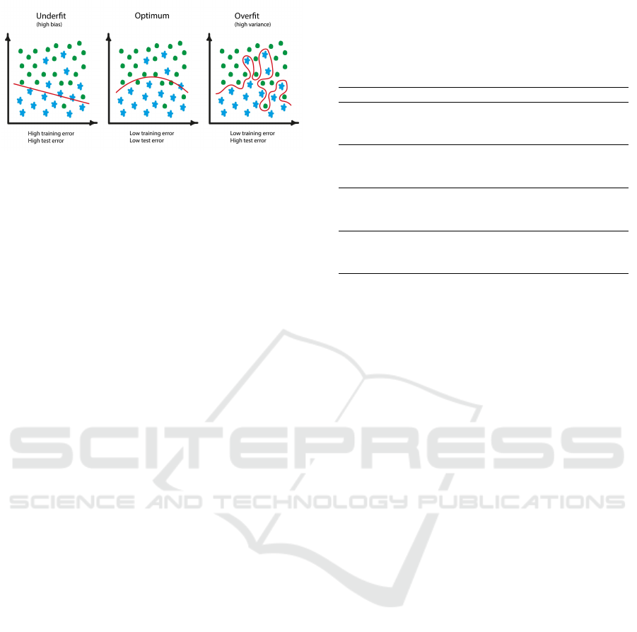
Figure 2: Visualization of underﬁtting versus overﬁtting.

As the model (represented as the red line) adapts further

to a certain set of data, the success towards the overall data

may decrease.

4 EXPERIMENTS AND RESULTS

This section will detail the various experimental ap-

proaches to the problem that this work presents. None

of the approaches employ a modiﬁcation of the net-

work used itself, instead preferring to work with the

parameters used in certain key points and the data

used. On the topic of data, all the experiments were

made using both the previously described datasets,

because the differences between them give important

insights to the problem at hand.

4.1 Depth Image Tests

The ﬁrst conditions are identical to the ones used by

Zhang et al. (Zhang et al., 2019a), simply to conﬁrm

that the results obtained are consistent with the results

presented by the authors, and give the initial baseline

to which all the following conditions will be com-

pared to. The optimization solver used is Stochastic

Gradient Descent (SGD) with a learning rate of 0.001

for both FeatherNet A and FeatherNet B with a decay

of 0.1 after every 60 epochs and a momentum setting

of 0.9, with FeatherNet A running for 200 epochs and

FeatherNet B for 150. The focal loss function is used

with α = 1 and γ = 3.

The results obtained with depth images are all

very successful and as such don’t leave much room

for improvement, they are in line with the results

presented by Zhang et al. (Zhang et al., 2019a), at

least where comparable. The only direct comparison

possible is between FeatherNet B with γ = 3 using the

CASIA-SURF dataset to which the result presented

was an ACER of 0.00971, most of the other results

presented were obtained with their proposed Multi-

Modal Face Dataset (MMFD) but have results in the

same ballpark. However, from table 3 it is already

possible to draw certain conclusions mostly about the

effects of the different datasets and the effects of the

Table 3: Results obtained from depth images. The best

epoch corresponds to the epoch that achieved the highest

accuracy, not the highest ACER. The value γ is the focusing

parameter used in focal loss function. B.E. stands for best

epoch and Acc. for accuracy.

Model Dataset γ B.E. Acc. ACER

2 4 99.063 0.008

FeatherNet A CASIA-SURF 3 4 99.323 0.007

5 4 98.886 0.012

2 4 99.386 0.005

FeatherNet B CASIA-SURF 3 5 99.042 0.010

5 12 99.178 0.007

2 16 99.972 0.0005

FeatherNet A WMCA 3 57 99.958 0.0004

5 160 99.696 0.005

2 81 99.986 0.0003

FeatherNet B WMCA 3 49 99.958 0.0006

5 122 99.993 0.0001

focusing parameter, but these will be discussed

in detail once all the relevant results are presented.

4.2 Colour Image Tests

With the intent of eventually applying liveness de-

tection to everyday devices, there can’t be a reliance

in forms of information not attainable by said de-

vices. As such the models are retrained using the

RGB images present in the datasets. Again, since

both datasets were obtained using the same camera

there aren’t concerns about differences in quality that

could affect the results. Aside from the change in in-

formation fed to the model, all other conditions are

the same as the ones used initially.

Immediately noticeable in table 4 is the fact that

aside from the experiments using only the WMCA

dataset, none of the best epochs’ accuracy are ever

as high as the ones using depth images by margins of

around 10% while maintaining the fact that the best

accuracy is obtained in the very early epochs. This

could already hint at overﬁtting but is not a fair as-

sumption since the results of table 3 maintain those

high accuracy values for the remaining epochs, while

this is not the case for the RGB images.

With table 5 the hypothesis of overﬁtting is con-

ﬁrmed for all the experiments involving the CASIA-

SURF dataset while completely not present in the

WMCA experiments. From the very early best epoch

(when considering that the models run for 200 and

150 epochs) the suspicion of overﬁtting is already

present. The conﬁrmation comes when looking at

the accuracy values presented by the last epochs the

model ran, with the accuracy values of these epochs

being far lower than the one presented for the best

epoch.

ICPRAM 2023 - 12th International Conference on Pattern Recognition Applications and Methods

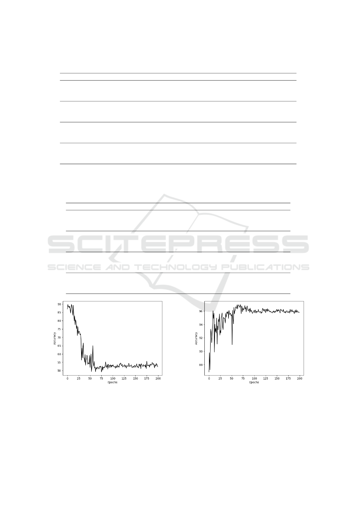
Table 4: Results obtained from RGB images. This table presents EER as an additional metric of success and also presents

APCER and BPCER as a means to check if the model fails more in recognising the attacks or the bonaﬁde cases.

Model Dataset γ B.E. EER Acc. APCER BPCER ACER

2 1 0.093 91.996 0.039 0.172 0.105

FeatherNet A CASIA-SURF 3 9 0.081 89.748 0.129 0.044 0.087

5 20 0.080 90.466 0.117 0.048 0.082

2 12 0.093 89.675 0.117 0.073 0.095

FeatherNet B CASIA-SURF 3 3 0.093 91.674 0.068 0.117 0.092

5 19 0.067 92.038 0.093 0.049 0.071

2 16 0.0005 99.972 0.0001 0.001 0.0005

FeatherNet A WMCA 3 69 0.043 96.988 0.024 0.051 0.038

5 160 0.004 99.696 0.001 0.008 0.005

2 81 0.0005 99.986 0.000 0.005 0.0003

FeatherNet B WMCA 3 63 0.026 98.529 0.009 0.033 0.021

5 122 0.0003 99.993 0.000 0.0003 0.0001

Table 5: Average of the 50 last epochs obtained from RGB images. This table presents the averages of the last 50 epochs of

each test (epoch 149-199 for FeatherNet A and epoch 99-149 for FeatherNet B) as to display at which values the model settles.

The standard deviation of the accuracy average is displayed as to observe the consistency of the results and the APCER and

BPCER averages are presented as to be compared to the ones of the best epoch for each experiment to draw conclusions on

what is the class with more classiﬁcation errors.

Model Dataset γ Avg. Acc. Std. APCER Avg. BPCER Avg.

2 52.306 0.888 0.692 0.002

FeatherNet A CASIA-SURF 3 53.179 0.877 0.679 0.002

5 60.866 1.422 0.566 0.004

2 56.582 1.275 0.630 0.002

FeatherNet B CASIA-SURF 3 58.762 1.170 0.598 0.001

5 57.667 1.328 0.614 0.002

2 99.392 0.061 0.005 0.010

FeatherNet A WMCA 3 95.984 0.165 0.032 0.067

5 99.449 0.085 0.005 0.008

2 99.868 0.073 0.001 0.001

FeatherNet B WMCA 3 97.479 0.298 0.015 0.060

5 99.917 0.089 0.001 0.0003

Figure 3: Results obtained with CASIA-SURF, RGB im-

ages, FeatherNetA and γ = 3.

Based on the accuracy scores, the use of RGB

images is a downgrade from the depth information,

more so when looking at the ﬁnal averages of the

model. This is not an issue of colour information per

Figure 4: Results obtained with WMCA, RGB images,

FeatherNetA and γ = 3.

se, but the lack of supervision from additional infor-

mation, as explained previously. There are some con-

clusions to be taken from, that while using RGB im-

ages, CASIA-SURF related experiments fail to main-

Dealing with Overﬁtting in the Context of Liveness Detection Using FeatherNets with RGB Images

tain the results obtained with depth images, WMCA

related experiments don’t, as shown in ﬁgures 3 and 4.

They will be taken in consideration when discussing

the differences between the two datasets, but for now,

explaining why CASIA-SURF fails to maintain re-

sults is quite simple.

Depth images are capable of giving information

that is not very perceptible otherwise, easily spotting

attacks that alter the depth of a regular face. Since

CASIA-SURF only presents print attacks, which con-

sist in covering an individual’s face with a sheet of pa-

per (as far as a depth image is concerned), the model’s

capability for distinguishing between the two cases is

very high. However if the model only has the RGB

images, and supposing that the quality of the print is

very high, an image of someone’s face and an image

of someone holding someone else’s picture might not

be as distinguishable and this problem is exacerbated

if the image is cropped.

Figure 5: Comparison between RGB and depth images of

a print attack (left) and a bonaﬁde face (right). Note that

the depth images aren’t of great quality, not being able to

capture the eyes cut out of the print attack and not giv-

ing much detail to the bonaﬁde case, but being possible to

notice the differences. Images selected from the CASIA-

SURF dataset (Zhang et al., 2019b).

4.3 Cross Dataset Tests

Cross dataset testing, as the name might suggest, sim-

ply entails in testing the model on a different dataset

than the one that was use in its training. Being already

aware of the differences between CASIA-SURF and

WMCA, cross dataset testing was used to check how

the model succeeded and how the larger variety of

spoofs affects the results, being trained in CASIA-

SURF and tested on WMCA and then vice versa.

To further observe how more spoofs affect a

model’s performance, a ”new” dataset ”GRAFTSET”

was created by adding, to the initial CASIA-SURF,

spoof cases from WMCA. Only Replay and Mask at-

tacks were added being that Print attacks are already

prevalent in CASIA-SURF as it is, and were added by

1%, 5% and 10% of the number of ﬁles of CASIA-

SURF, initially with only one type of attack added,

The name was chosen from the botanical activity of

grafting which consists of joining tissues of different plants,

for example a branch from an olive tree to the trunk of an

apple tree. In this analogy CASIA-SURF is the trunk, and

the selected attacks from WMCA are the branches.

and then both at the same time. With the new dataset

constructed, new cross dataset tests were conducted,

with training being done with the GRAFTSETS and

testing on WMCA.

Explaining why WMCA shows no overﬁtting at

all while CASIA-SURF’s poor ﬁnal averages indicate

that overﬁtting occurred, consists basically in the fact

that even though the problem is still approached with

a binary point of view, there is a larger distinction be-

tween the bonaﬁde cases, which the model is trying to

categorize as such, and the attacks that between them

have more variability.

To emphasize the effects of more attacks we

analyze the results obtained from the cross-dataset

tests which include not only the ones with the basic

CASIA-SURF and WMCA but also the ones involv-

ing the various GRAFTSETs. The results from the

initial cross dataset tests are almost identical to the re-

sults obtained from the intra dataset experiments, this

of course since the training set is maintained and only

the testing set is changed. A more diverse training is

bound to achieve better results, in fact, Liu et al. de-

veloped their dataset SiW-M with 13 different spoof

types with the intent of training models to be able

to then correctly identify different attack types not

present in the initial training set. It is from these con-

clusions that the idea for the GRAFTSET tests take

place, by adding different spoof cases to the training

set of CASIA-SURF there is a slight improvement to

the ﬁnal average of the last epochs of the model. The

inclusion of just one type of attack or both achieve

similar results in terms of just the average, but having

both types of attacks reduces the standard deviation

indicating more consistent results.

4.4 Focus Parameter Tests

These experiments entail an ablation study of the fo-

cusing parameter, which is initially decreased to 2 and

increased to 5 in order to take note on how it affects

the results. These values were chosen from the ones

used by Lin et al. (Lin et al., 2020) being the ones

closest to the one used by Zhang et al. (Zhang et al.,

2019a).

The discrepancy between the APCER averages

and the BPCER averages has to be addressed. For

most experiments, while the BPCER averages are

quite low showing very few cases of bonaﬁde cases

being labelled as spoofs, the APCER averages are

very high reaching values above 50%. This can be

considered the worst case scenario since if hypothet-

ically this model would be used for a security oper-

ation, an unauthorized access would be made. If the

values were inverted with very high BPCER and low

ICPRAM 2023 - 12th International Conference on Pattern Recognition Applications and Methods

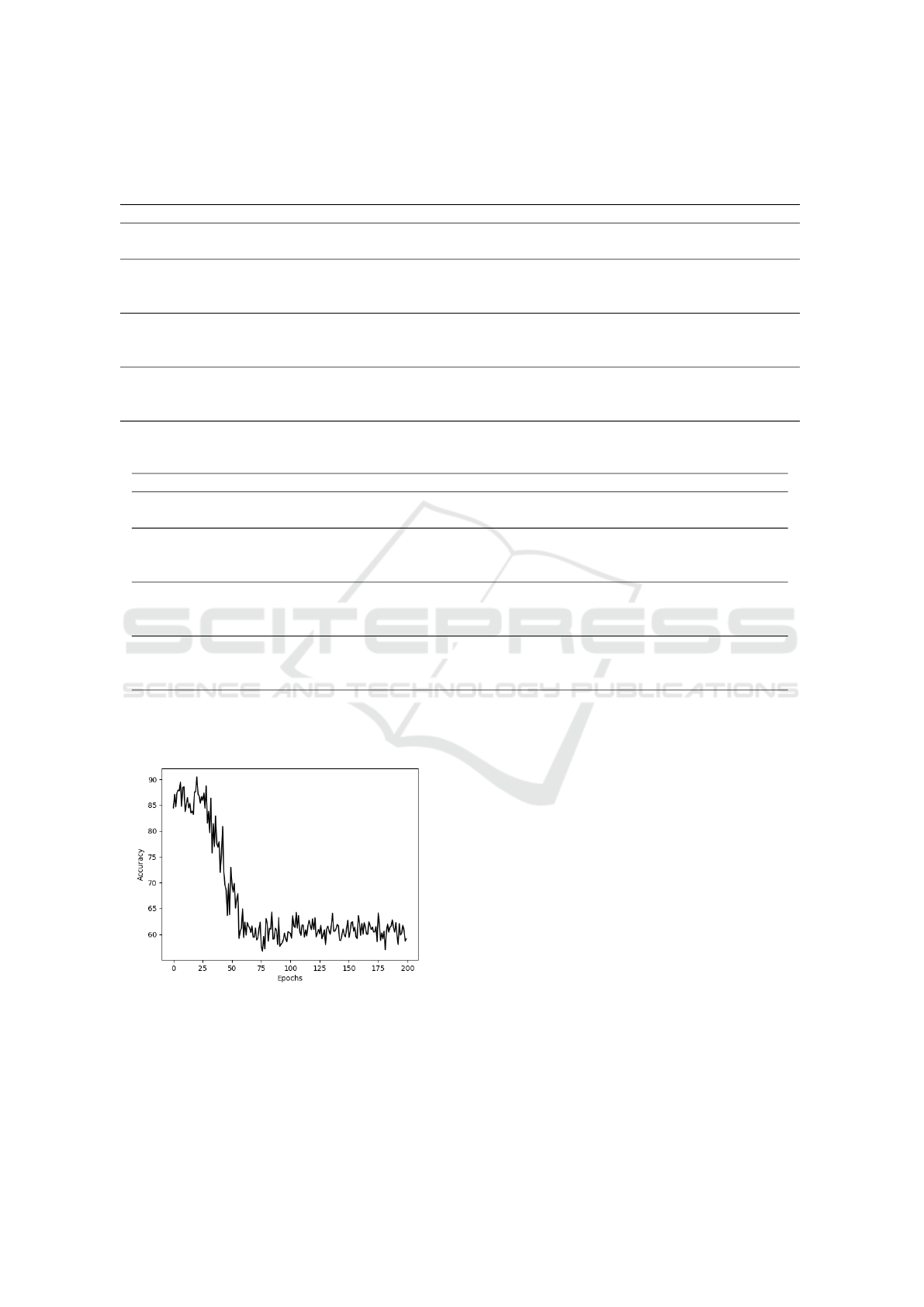
Table 6: Results obtained from cross dataset testing. The ﬁrst two results are the obtained from the unaltered datasets with the

ﬁrst name presented being the train set and the second the test set. Important to note that the ”GRAFTSET” tests are all cross

dataset tests with the training with GRAFTSET and testing with WMCA.

Model Dataset γ B.E. EER Acc. APCER BPCER ACER

FeatherNet A CASIA-SURF - WMCA 3 1 0.107 90.477 0.050 0.195 0.122

FeatherNet A WMCA - CASIA-SURF 3 56 0.032 97.635 0.019 0.039 0.029

GRAFTSET - 1% Replay 5 0.104 90.416 0.084 0.122 0.103

FeatherNet A GRAFTSET - 5% Replay 3 11 0.080 89.91 0.126 0.044 0.085

GRAFTSET - 10% Replay 7 0.089 90.674 0.102 0.072 0.087

GRAFTSET - 1% Mask 5 0.087 89.489 0.125 0.061 0.093

FeatherNet A GRAFTSET - 5% Mask 3 18 0.083 88.828 0.144 0.035 0.090

GRAFTSET - 10% Mask 2 0.106 88.594 0.124 0.091 0.107

GRAFTSET - 1% Both 0 0.145 87.776 0.069 0.243 0.156

FeatherNet A GRAFTSET - 5% Both 3 9 0.065 89.913 0.131 0.025 0.078

GRAFTSET - 10% Both 3 0.087 91.62 0.080 0.094 0.090

Table 7: Average of the 50 last epochs obtained from cross dataset tests. The observations made referencing the naming and

the presence of certain values, in both table 5 and 6 are valid for this table.

Model Dataset γ Avg. Acc. Std. APCER Avg. BPCER Avg.

FeatherNet A CASIA-SURF - WMCA 3 53.272 0.870 0.678 0.001

FeatherNet A WMCA - CASIA-SURF 3 96.479 0.250 0.032 0.046

GRAFTSET - 1% Replay 53.863 0.725 0.666 0.002

FeatherNet A GRAFTSET - 5% Replay 3 59.541 1.017 0.574 0.004

GRAFTSET - 10% Replay 59.117 2.061 0.569 0.007

GRAFTSET - 1% Mask 52.679 0.853 0.684 0.001

FeatherNet A GRAFTSET - 5% Mask 3 55.249 0.829 0.635 0.003

GRAFTSET - 10% Mask 59.497 6.063 0.568 0.009

GRAFTSET - 1% Both 55.048 0.695 0.647 0.001

FeatherNet A GRAFTSET - 5% Both 3 58.647 0.761 0.577 0.001

GRAFTSET - 10% Both 59.471 0.492 0.553 0.003

APCER, legitimate users would be barred from ac-

cess but very few successful attacks could occur, a far

too restrictive system but secure nonetheless.

Figure 6: Results obtained with CASIA-SURF, RGB im-

ages, FeatherNetA and γ = 5.

Since Focal Loss results in a model that is more

focused in the spoof cases and won’t learn as much

from what would be considered a bonaﬁde one, it

would be expected that it would be able to more suc-

cessfully categorize spoofs as such. The reality is

that through the differences explained in the transi-

tion from depth images to colour images, the RGB

spoofs don’t offer as much as the depth ones and as

a consequence, the ”focus” is squandered. Reducing

the focusing parameter doesn’t appear to have much

effect on overﬁtting but increasing it does seem to de-

lay it slightly, as is noticeable when comparing ﬁgures

3 and 6.

To conﬁrm this observation, it’s only required to

further reduce the focusing parameter, eventually re-

moving the modulating factor with γ = 0. Tables 8 and

9 display these results that when compared to their

counterparts using the same datasets and model, are

pretty much the same without much improvement or

degradation. There is however an observation to be

made that without the focusing parameter, the model

is still able to achieve great results on the WMCA

dataset further solidifying the conclusion that with

more variability within a dataset, there is less need

to implement precautions against overﬁtting.

Dealing with Overﬁtting in the Context of Liveness Detection Using FeatherNets with RGB Images

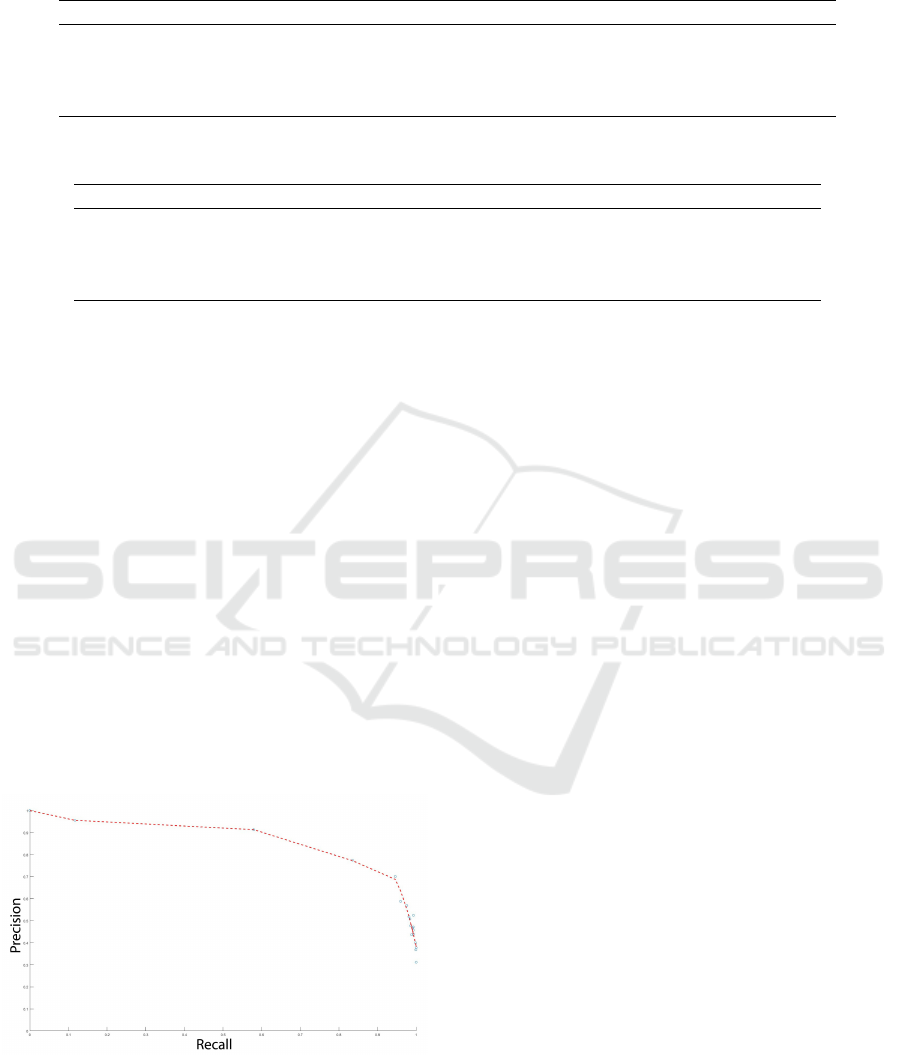
Table 8: Results obtained with γ = 0 and γ = 1. With the focusing parameter turned to 0, the model is no longer using focal

loss but simply a weighted version of binary cross-entropy.

Model Dataset γ B.E. EER Acc. APCER BPCER ACER

FeatherNet A CASIA-SURF 0 1 0.094 91.07 0.078 0.115 0.096

1 1 0.095 91.861 0.035 0.184 0.110

FeatherNet A WMCA 0 108 0.009 99.153 0.009 0.007 0.008

1 47 0.022 98.8 0.0005 0.051 0.026

Table 9: Average of the 50 last epochs obtained with γ = 0 and γ = 1. These results are presented to comment on how these

changes affect overﬁtting.

Model Dataset γ Avg. Acc. Std. APCER Avg. BPCER Avg.

FeatherNet A CASIA-SURF 0 51.705 0.571 0.701 0.012

1 55.466 0.686 0.646 0.001

FeatherNet A WMCA 0 98.766 0.148 0.012 0.013

1 97.474 0.210 0.022 0.037

4.5 Precision Recall Tests

To construct the precision-recall (PR) curve, the ap-

proach is running the model at different thresholds

between 1, where no image can be considered as

bonaﬁde and 0 where all predictions will be bonaﬁde.

Once all these values are obtained the points can be

plotted in a graph and then a curve adjusted to them.

From this curve a point can be picked out as what is

considered ideal, in this case the closest point to what

be considered perfect i.e. (precision, recall) = (1, 1),

however the threshold value needs to be inferred from

where the ideal point stands in the graph. This ab-

lation study was conducted using the CASIA-SURF

dataset on FeatherNet A with γ = 3 with the thresh-

old values being selected as the experiments went on

attempting to achieve the most interesting PR curve.

These values and the resulting precision and recall

values are presented in table 10 and result in the curve

presented in ﬁgure 7.

Figure 7: Precision-Recall curve. The curve was ob-

tained using Matlab’s polyﬁt() function. The threshold cho-

sen was obtained by using Euclidean distance to ﬁnd the

closest point to the perfect (1,1) which resulted in point

(0.8913,0.7828) which corresponds to a threshold value of

roughly 0.9675.

4.6 Final Tests

With the ”ideal” threshold calculated threshold =

0.9675, it is only a matter of repeating the initial ex-

periments of interest with this new value and see if it

improves and how.

Immediately noticeable is how the best epoch oc-

curs later over the 200 epochs of FeatherNet A which

should already indicate some amount of success in re-

ducing overﬁtting but is of course not a guaranteed

conclusion. Also noticeable is when the model is

tested on WMCA there are no false positive predic-

tions, demonstrated by APCER = 0, while also in-

creasing the false negative cases since the BPCER

value increased by quite a lot. Considering such a

high threshold value this makes sense, but demon-

strates that for different datasets, different PR curves

should be calculated since the ”ideal” threshold will

most certainly vary between them. To conﬁrm if there

is no overﬁtting, once again, the average values of the

last epochs are presented.

The high averages presented in table 12 conﬁrm

that, in fact, no overﬁtting has occurred, but the higher

standard deviation also indicates that while overall

these results can be considered satisfactory, there is

a certain degree of variability to the model’s results

that needs to be considered. The most ”stable” and

improved results come from the GRAFTSET exper-

iment which maintains the close results during the

later epochs as demonstrated by the lower standard

deviation that was only noted when the dataset in-

cluded both extra spoof types and achieving a lower

APCER than BPCER.

Overall, the adaptation of the threshold that deter-

mines what prediction is made, resulted in the con-

siderable decrease of the overﬁtting when it was pre-

viously presented, while unfortunately giving worse

results for the cases where there was no previous over-

ICPRAM 2023 - 12th International Conference on Pattern Recognition Applications and Methods

Table 10: Values used to obtain the Precision-Recall curve. Note that for threshold = 1 the precision formula results in

a division by 0 and as such would not be valid, the 100% precision comes from the interpretation that since no positive

classiﬁcations were made, technically none of them are wrong. The TN, FP, FN and TP values were not obtained from the

best epoch but from the average of the ﬁnal 50 results, as to keep consistency in analyzing the overﬁtting effect.

Threshold TN FP FN TP Precision Recall Accuracy

1 6614 0 2994 0 1.000 0.000 68.838

0.99 6587.8 16.2 2644.04 349.96 0.956 0.117 72.312

0.9825 6448.5 165.5 1258.9 1735.1 0.913 0.580 85.175

0.975 5886.12 727.88 493.22 2500.78 0.775 0.835 87.291

0.95 5405.44 1208.56 161.9 2832.1 0.701 0.946 85.736

0.925 4601.4 2012.6 120.64 2873.36 0.588 0.960 77.797

0.9 4401.98 2212.02 73.04 2920.96 0.569 0.976 76.217

0.875 3880.28 2733.72 55.9 2938.1 0.518 0.981 70.966

0.85 3760.78 2853.22 47.66 2946.34 0.508 0.984 69.808

0.825 3233.82 3380.18 27.82 2966.18 0.467 0.991 64.530

0.8 3922.44 2691.56 20.66 2973.34 0.525 0.993 71.771

0.7875 3382.96 3231.04 43.02 2950.98 0.477 0.986 65.924

0.775 3282.98 3331.02 22.06 2971.94 0.472 0.993 65.101

0.75 3088.64 3525.36 21.4 2972.6 0.457 0.993 63.085

0.71 2797.72 3816.28 34.48 2959.52 0.437 0.988 59.921

0.67 2805.36 3808.64 20.62 2973.38 0.438 0.993 60.145

0.5 2120.22 4493.78 4.74 2989.26 0.399 0.998 53.179

0.33 1682.02 4931.98 0 2994 0.378 1.000 48.668

0.25 1482.88 5131.12 1.92 2992.08 0.368 0.999 46.577

0 0 6614 0 2294 0.312 1.000 31.161

Table 11: Results obtained with the ﬁnal threshold. All these experiments were conducted in the same conditions as previously

only changing the threshold used.

Model Dataset γ B.E. EER Acc. APCER BPCER ACER

FeatherNet A CASIA-SURF 3 36 0.117 89.373 0.049 0.232 0.141

FeatherNet A GRAFTSET - 10% Both 3 59 0.110 90.377 0.046 0.217 0.131

FeatherNet A WMCA 3 189 0.018 91.165 0 0.385 0.193

ﬁtting, keeping in mind that if the threshold tuning

was made with WMCA this would not happen but

most likely the improvement for the other two would

not be so good or would not occur.

5 CONCLUSION AND FUTURE

WORKS

With machine learning being used ever more often for

liveness detection solutions, it comes with the prob-

lem of overﬁtting where the model adapts to data

incorrectly due to outliers or a minimal set of data.

While there are several approaches to attempt to re-

duce the overﬁtting effect, these are usually made at

an implementation level directly on the model that is

constructed. This paper presented some alternatives

more focused in the input and output of the model by

approaching the datasets used for the input and the

loss function and how the output is interpreted.

These alternatives showed the importance of a var-

ied dataset and how these variations are able to com-

pensate for loss of information associated with the

multiple modalities an image can be presented with.

From this loss of information, the overﬁtting effect

present in the model became considerably noticeable

with a difference between the best result, obtained at

epoch 9 with an accuracy of 89.75%, and the average

accuracy of the last ﬁfty epoch’s, equal to 36.57%. By

adjusting the threshold that deﬁned bonaﬁde or spoof,

this difference was reduced to 3.63%.

The results obtained during this work present pos-

sible considerations that could be helpful in the devel-

opment of future solutions, both regarding the size,

diversity and applicability of the datasets, as well as

the modality given to the model. One of the con-

clusions that was met is the importance of diverse

datasets, which entails that a great beneﬁt to the com-

munity would be the development of a dataset that

could boost both the quality and dimension of the

CASIA-SURF dataset with the number of diverse

Dealing with Overﬁtting in the Context of Liveness Detection Using FeatherNets with RGB Images

Table 12: Average of the 50 last epochs obtained with the ﬁnal threshold. These results are presented to comment on how

these changes affect overﬁtting.

Model Dataset γ Avg. Acc. Std. APCER Avg. BPCER Avg.

FeatherNet A CASIA-SURF 3 85.746 1.003 0.160 0.105

FeatherNet A GRAFTSET - 10% Both 3 87.478 0.401 0.113 0.155

FeatherNet A WMCA 3 88.446 1.012 0 0.504

cases both in presentation attacks and ambient condi-

tions of WMCA. Not only would this dataset be much

closer to what a real day-to-day use of a PAD appli-

cation would encounter, it would also beneﬁt the gen-

eralization of models developed with it. Hence mean-

ing, that with a more diverse dataset, the number of

studies that deviate from the binary approach to live-

ness detection by categorizing each attack individu-

ally could grow with different insights on what dif-

ferent attacks are more challenging with what modal-

ities.

On a ﬁnal note, and trying to be straightforward

on the best approach regarding the information given

to the model, on a regular application, the conclusion

was moving away from depth or infra red, on both

direct input, or only as a supervision for the model,

as well as sticking with the regular color informa-

tion, proving that the way the model is constructed

is of great importance. The building of a new model

that, like FeatherNets, tries to be as light as possible,

achieving great results and not requiring extra infor-

mation could beneﬁt from some of the considerations

made here. This model would require a new approach

to its construction since many of the choices made

for FeatherNets were taken considering the depth in-

put. Since this new theoretical model would return

to the more common use RGB images but forego the

supervision provided by the extra modalities (depth,

infra red), techniques that were successful for these

types of models might not beneﬁt this one, being per-

haps beneﬁcial to consider the approaches used before

the extra modalities were available while considering

not only the more complex dataset as well as the ap-

proaches demonstrated in this paper.

REFERENCES

Atoum, Y., Liu, Y., Jourabloo, A., and Liu, X. (2017). Face

anti-spooﬁng using patch and depth-based cnns. 2017

IEEE International Joint Conference on Biometrics

(IJCB), pages 319–328.

Chingovska, I., Anjos, A. R. d., and Marcel, S. (2014).

Biometrics evaluation under spooﬁng attacks. IEEE

Transactions on Information Forensics and Security,

9(12):2264–2276.

George, A., Mostaani, Z., Geissenbuhler, D., Nikisins, O.,

Anjos, A., and Marcel, S. (2020). Biometric face pre-

sentation attack detection with multi-channel convo-

lutional neural network. IEEE Transactions on Infor-

mation Forensics and Security, 15.

Hao, H., Pei, M., and Zhao, M. (2019). Face liveness detec-

tion based on client identity using siamese network.

Pattern Recognition and Computer Vision: Second

Chinese Conference, PRCV 2019, pages 172–180.

He, K., Zhang, X., Ren, S., and Sun, J. (2016). Deep resid-

ual learning for image recognition. 2016 IEEE Con-

ference on Computer Vision and Pattern Recognition

(CVPR), pages 770–778.

Janocha, K. and Czarnecki, W. M. (2017). On loss func-

tions for deep neural networks in classiﬁcation. Pro-

ceedings of the Theoretical Foundations of Machine

Learning 2017 (TFML 2017).

Kim, T., Kim, Y., Kim, I., and Kim, D. (2019). Basn: En-

riching feature representation using bipartite auxiliary

supervisions for face anti-spooﬁng. 2019 IEEE/CVF

International Conference on Computer Vision Work-

shop (ICCVW), pages 494–503.

Lin, T. Y., Goyal, P., Girshick, R., He, K., and Dollar, P.

(2020). Focal loss for dense object detection. IEEE

Transactions on Pattern Analysis and Machine Intel-

ligence, 42.

Liu, Y., Stehouwer, J., Jourabloo, A., and Liu, X. (2019).

Deep tree learning for zero-shot face anti-spooﬁng.

Proceedings of the IEEE Computer Society Confer-

ence on Computer Vision and Pattern Recognition,

2019-June.

Menotti, D., Chiachia, G., Pinto, A., Schwartz, W. R.,

Pedrini, H., Falcao, A. X., and Rocha, A. (2015).

Deep representations for iris, face, and ﬁngerprint

spooﬁng detection. IEEE Transactions on Informa-

tion Forensics and Security, 10:864–879.

Sandler, M., Howard, A., Zhu, M., Zhmoginov, A., and

Chen, L.-C. (2018). Mobilenetv2: Inverted residuals

and linear bottlenecks. 2018 IEEE/CVF Conference

on Computer Vision and Pattern Recognition, pages

4510–4520.

Sun, W., Song, Y., Chen, C., Huang, J., and Kot, A. C.

(2020). Face spooﬁng detection based on local ternary

label supervision in fully convolutional networks.

IEEE Transactions on Information Forensics and Se-

curity, 15:3181–3196.

Wayman, J. L. (2007). 10 - the scientiﬁc development of

biometrics over the last 40 years. In Leeuw, K. D.

and Bergstra, J., editors, The History of Information

Security, pages 263–274. Elsevier Science B.V., Am-

sterdam.

Xu, X., Xiong, Y., and Xia, W. (2020). On improving tem-

poral consistency for online face liveness detection.

arXiv preprints arXiv:2006.06756.

ICPRAM 2023 - 12th International Conference on Pattern Recognition Applications and Methods

Xu, Z., Li, S., and Deng, W. (2015). Learning tempo-

ral features using lstm-cnn architecture for face anti-

spooﬁng. 2015 3rd IAPR Asian Conference on Pattern

Recognition (ACPR), pages 141–145.

Yang, J., Lei, Z., and Li, S. Z. (2014). Learn convolutional

neural network for face anti-spooﬁng. arXiv preprints

arXiv:1408.5601.

Ying, X. (2019). An overview of overﬁtting and its solu-

tions. Journal of Physics: Conference Series, 1168.

Yu, Z., Qin, Y., Li, X., Zhao, C., Lei, Z., and Zhao, G.

(2021). Deep learning for face anti-spooﬁng: A sur-

vey. IEEE Transactions on Pattern Analysis and Ma-

chine Intelligence (TPAMI).

Yu, Z., Zhao, C., Wang, Z., Qin, Y., Su, Z., Li, X., Zhou,

F., and Zhao, G. (2020). Searching central differ-

ence convolutional networks for face anti-spooﬁng.

IEEE/CVF Conference on Computer Vision and Pat-

tern Recognition (CVPR), pages 5295–5305.

Zhang, P., Zou, F., Wu, Z., Dai, N., Mark, S., Fu, M.,

Zhao, J., and Li, K. (2019a). Feathernets: Convo-

lutional neural networks as light as feather for face

anti-spooﬁng. IEEE Computer Society Conference on

Computer Vision and Pattern Recognition Workshops,

2019-June.

Zhang, S., Wang, X., Liu, A., Zhao, C., Wan, J., Escalera,

S., Shi, H., Wang, Z., and Li, S. Z. (2019b). A dataset

and benchmark for large-scale multi-modal face anti-

spooﬁng. Proceedings of the IEEE Computer Society

Conference on Computer Vision and Pattern Recogni-

tion, 2019-June.

Dealing with Overﬁtting in the Context of Liveness Detection Using FeatherNets with RGB Images