Head Star (H*): A Motion Planning Algorithm for Navigation Among

Movable Obstacles

Halim Djerroud

ESIEE Paris, Gustave Eiffel University, France

Keywords:

Motion Planning, Navigation Among Movable Obstacles, Bug Algorithms.

Abstract:

The objective of Navigation Among Movable Obstacles (NAMO) is to optimise the behaviour of robots by

giving them the ability to manipulate obstacles. Current NAMO methods use two planners, one for moving

through open spaces and a second for handling obstacles. However, these methods focus on providing a

solution for obstacles handling and neglect movement in free spaces. These methods usually assume using

classical obstacle avoidance algorithms for moving in free spaces. However, they are not suitable for the

NAMO. This paper proposes a new path planning algorithm Head Star (H*) adapted for NAMO in free spaces.

It is inspired by Bug’s algorithms by adding a graphical representation and heuristics on the distances allowing

it to bring the robot as close as possible to its goal while keeping in memory the areas already visited.

1 INTRODUCTION

Designing a robot that can navigate in a congested

environment and move obstacles in its path is a

ﬁeld that roboticis have been interested in for sev-

eral decades, known as Navigation Among Mov-

able Obstacles (NAMO) (Stilman and Kuffner, 2005).

NAMO is an important area of research in motion

planning in congested environments, as it gives mo-

bile robots a better ability to reason about the envi-

ronment and the possibilities of choosing which ob-

stacles to manipulate, in order to make their way

through (Charalampous et al., 2017). NAMO thus

makes it possible to solve problems that are difﬁcult

or even impossible to solve with a conventional ob-

stacle avoidance methods.

Current work in the NAMO ﬁeld can be divided

into two broad categories: off-line planning and on-

line planning (Moghaddam and Masehian, 2016; Re-

nault et al., 2019). Ofﬂine planning assumes that all

the information of the space in which the robot is

moving is known in advance, while in contrast to on-

line planning, the robot has only partial knowledge of

its environment, and it can modify its initial plan ac-

cording to new information acquired during its move-

ment. In most previous work that has focused on of-

ﬂine NAMO, the results show that this approach is not

effective. The current trend is towards online NAMO,

which seems to be more promising and better suited.

There is not much work on online NAMO, but the

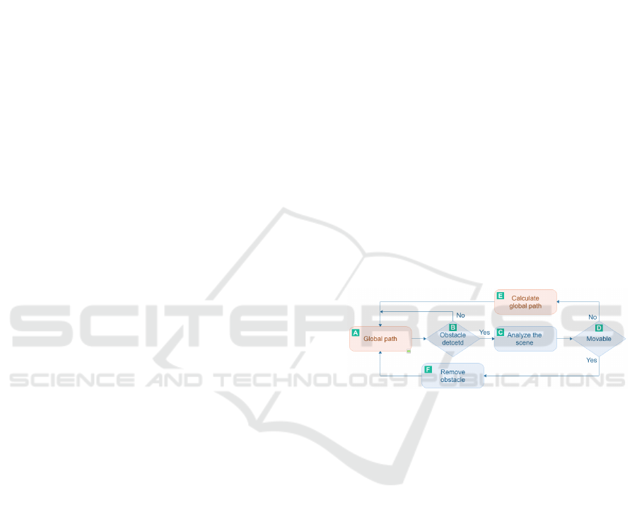
Figure 1: Overview of a method for solving NAMO: (A)

From a map of the environment the algorithm ﬁrst calcu-

lates a collision-free path to its goal. (B) During the execu-

tion of this path, the robot continuously searches for obsta-

cles not recorded in the map that may block its path. (C) If

such an obstacle is detected, the robot initiates a scene anal-

ysis to determine the mobility of the obstacles. (D) In case

the obstacle is not removable, then (E) the robot re-plans its

path. Otherwise (F) the robot removes the obstacle.

article (Renault et al., 2019) gives an almost exhaus-

tive list of algorithms with a classiﬁcation according

to the type of NAMO used. The approaches online

are those whose mobility is not given in the Table 1 in

(Renault et al., 2019)

In most of the approaches the authors use two

planners, one for the movement in free spaces to cal-

culate an optimal path and a second one for the han-

dling of obstacles. According to our knowledge the

set of proposed approaches focuses on the operation

of the planner that handles obstacles. For what con-

cerns the global planner that allows to compute a path

in free spaces the authors only assume that those plan-

ners uses a motion planning classical algorithm. This

Djerroud, H.

Head Star (H*): A Motion Planning Algorithm for Navigation Among Movable Obstacles.

DOI: 10.5220/0011637200003393

In Proceedings of the 15th International Conference on Agents and Artiﬁcial Intelligence (ICAART 2023) - Volume 3, pages 211-219

ISBN: 978-989-758-623-1; ISSN: 2184-433X

 2023 by SCITEPRESS – Science and Technology Publications, Lda. Under CC license (CC BY-NC-ND 4.0)

211

article seeks to resolve this lacking by proposing an

alternative path planning algorithm for NAMO.

In order to illustrate how the two planner meth-

ods work, we propose the diagram in Figure 1 which

proposes a method for solving NAMO whose objec-

tive is to lead the robot to a determined position by

manipulating the obstacles that hinder its passage. In

this method two planners are assumed, the ﬁrst one

(red rectangles) allows movement in free spaces. The

second one (blue rectangles) allows the management

of obstacles. In this proposal, the method consists of

bringing the robot as close as possible to its objective.

If a non-removable obstacle is in the proposed path

then a new path is calculated.

In order to achieve an efﬁcient global planner we

believe it is important to use a path calculation algo-

rithm adapted to NAMO, because classical planning

algorithms will try to ﬁnd a path assuming that all ob-

stacles are impassable. In the case of NAMO with a

global planner, to calculate an optimal path it is nec-

essary to try to bring the robot as close as possible to

its objective, even if it means ﬁnding itself in a block-

ing position, as long as the local planner can unblock

the situation by moving the obstacles.

In this paper we propose a motion planning algo-

rithm adapted for NAMO. The objective of this algo-

rithm is to bring the robot as close as possible to its

goal to allow an obstacle manager to remove obstacles

that hinder the passage. The algorithm also allows a

new path to be calculated quickly and taking into ac-

count the areas already explored in the event that the

local planner fails to ﬁnd a solution in the event of a

blockage.

In the following we will describe the existing mo-

tion planning algorithms and show the limitations of

these algorithms for NAMO. Afterwards we will pro-

pose a motion planning algorithm for NAMO under

the name of HeadStar (H*). Then, we will show the

experiments carried out prior to concluding.

2 OVERVIEW OF MOTION

PLANNING METHODES

Motion planning is an important step to address

NAMO problem. It allows the robot to ﬁnd a se-

quence of valid conﬁgurations which allow it to move

from a start position A to reach a goal B even if this

means ﬁnding itself in a blocked position.

In conventional navigation, all obstacles are as-

sumed to be impassable. This problem is known in

robotics under the term of motion planning. Histori-

cally, it was described in (Eiben and Kanj, 2017) also

called piano movers problem. It stipulates that if a

robot in an initial position and orientation wants to

move towards a ﬁnal position and orientation, there

must be at least one valid path between these two po-

sitions. A movement is said to be valid if it is car-

ried out completely without collision. Motion plan-

ning, therefore, consists in ﬁnding a valid trajectory

between two positions. A motion planning method

must: either generate a movement such that the robot

can reach the ﬁnal position without colliding with ob-

stacles, or conclude that such a movement is impossi-

ble.

Motion planning algorithms, described in

(LaValle, 2006) are divided into two main classes:

(1) deterministic methods, also called exact methods,

which make it possible to ﬁnd the same path at each

execution for a given conﬁguration of the environ-

ment. (2) Probabilistic methods, also called sampling

methods, on the other hand, can ﬁnd different paths

for the same initial conditions, but they guarantee

ﬁnding a solution if it exists, or to determine that a

solution is deﬁnitely nonexistent.

The solutions provided by the ﬁrst class of algo-

rithms are based on the topology of the free spaces

called also conﬁguration spaces, in order to build a

graph. So they consist in reducing the problem to a

simple path ﬁnding in a graph. The technique takes

place in two steps: The ﬁrst consists of construct-

ing a graph conforming to the conﬁguration space.

The second step uses algorithms for ﬁnding paths in a

graph, for example: Di jkstra, A∗, Bellman, D ∗Lite,

etc. As for the step of construction of the graphs, it is

based on a cells division method.

Among these techniques of cell division, one of

them consists of dividing the conﬁguration space into

a set of square cells. In this technique it is considered

that each cell is linked to the eight neighbouring cells.

All the cells can be represented in the form of a graph.

The cells represent the nodes, and the passages from

one cell to another are represented by weighted edges

as follows: The passages from one cell to another ver-

tically or horizontally is weighted at 1, diagonal pas-

sages are weighted at

√

2. If the cell represents an ob-

stacle, then the edges towards this cell are weighted

to inﬁnity.

The methods presented here (the list is not exhaus-

tive, we have only cited the most widespread methods

involved in this article) are so-called exact methods;

they have the advantage of working well for a robot

in the conﬁguration space C = R

. They are generally

based on graphs, so it is easy to calculate the prop-

erties (example: the shortest path, the total cost, etc.)

They also offer certain theoretical guarantees (com-

pleteness, limits on the execution time, etc.) But these

methods are only used when the environment and the

ICAART 2023 - 15th International Conference on Agents and Artiﬁcial Intelligence

212

obstacles are known (or partially known on condition

that certain algorithms such as D ∗Lite (Koenig and

Likhachev, 2002) are used for example) in advance

and can be very slow if the number of dimensions is

greater than two.

Another category of algorithms, called probabilis-

tic algorithms, is based on the use of randomness to

construct a connected graph in a conﬁguration space,

thus allowing it to be freed from an exact represen-

tation of the environment. These methods perform

a random search in free space until the desired ﬁ-

nal conﬁguration is reached. Among these methods

we ﬁnd the Probabilistic Roadmap Approach (PRM)

(Chen et al., 2021). As previously, the technique con-

sists of two phases. The ﬁrst phase in the construction

of a graph (this phase is called learning phase) and

the second, (called research phase), consisting of the

search for a path in this graph. The graph represents

the free space. To ensure a total exploration of the

free space, each node of the graph is drawn randomly

according to a uniform distribution. Each time a node

is randomly pulled it is veriﬁed as to whether or not

there is a straight line without collision with the nodes

closest to the graph, which respects the constraints of

the mobile. If this condition is veriﬁed, then we add

this new node to the graph and connect it to the clos-

est nodes. There are several variants of this algorithm.

Among them, Rapidly exploring Roadmap Random

Trees (RRT) (LaValle et al., 1998; Kalpitha et al.,

2020), which is based on the same technique but al-

lows convergence more quickly by choosing only the

nodes which are relevant to the solution of the prob-

lem, resulting in the reduction of computation time.

From the initial position of the mobile, a tree is suc-

cessively constructed by successive integration of the

nodes. To create a new node, we generate a random

sample of the conﬁguration space that we will call

rand using a random distribution to maximise explo-

ration. The near node closest to rand is determined,

and a new candidate conﬁguration new then produces

a segment joining near to rand, at a distance preﬁxed

δ from near. Finally, we check that the segment from

near to new is collision-free. If this condition is true,

we add new to the graph and connect it with a segment

near to new.

Another class of algorithms, which allows robots

to blindly navigate in mapless environments, is com-

monly known as Bug Algorithms (BA). As the name

suggests, they have a biological origin. They are

based upon techniques inspired by the movement of

insects. A description and comparison of a wide vari-

ety of these algorithms can be found in the following

articles : (McGuire et al., 2019) (Sivaranjani et al.,

2021). The principle of these algorithms is that they

do not know the position of the obstacles in their en-

vironment, nor the relative position of the goal to be

reached. They will react locally only to contact with

obstacles and walls which constitute their immediate

environment so as to allow the robot to progress to-

wards its objective by following the limits of the ob-

stacles and walls. The nature of these algorithms is

ideal for indoor navigation, where the map of the en-

vironment is not known in advance, and/or the struc-

ture of the environment is constantly changing. The

Bug Algorithms are based on the following criteria:

(1) Unlike many planning algorithms, which assume

a global knowledge of the environment, these algo-

rithms assume only a local knowledge of the environ-

ment and a global objective. (2) Their behaviour is

straightforward: (a) follow the contours of obstacles

(b) move in a straight line towards the objective. (3)

The range of the sensors is limited and admits a cer-

tain range of uncertainty of the ﬁnal position. The

typical behaviour of Bug Algorithms is to move in a

direct line whenever possible, until reaching the goal.

In case the mobile meets an obstacle it follows the

contour of the obstacle until it is possible to go in a

straight line towards the goal.

Among the simplest algorithms, we ﬁnd the Com

(Lumelsky and Stepanov, 1986) algorithms they have

been qualiﬁed by the authors of (McGuire et al., 2019)

as common sense algorithms and they have abbrevi-

ated them under the acronym Com. The idea is to

move in a direct line whenever possible, until waiting

for the goal. In case the mobile meets an obstacle then

it follows the contour of the obstacle until it is possi-

ble to go in a straight line towards the goal. The ﬁrst

point of contact with the obstacle is called hit-point,

and the point where the mobile leaves the outline of

the obstacle to go in a straight line towards the goal

is called leave-point. This algorithm can solve sev-

eral situations, but the authors show some problem-

atic cases shown in Figure 2 (a). To solve the prob-

lem posed by Com the authors suggest the Bug1 al-

gorithm which proposes to explore the totality of the

obstacle while keeping the last point leave-point in

its memory as shown in Figure 2 (b). However Bug1

generally proposes a path for this, the authors propose

an optimized version of this algorithm, named Bug2

whose idea consists in drawing an imaginary line M-

line between the starting position and the goal. Bug1

explores the obstacle but this time, until we encounter

the M-line, this situation is illustrated in Figure 2 (c).

In the same article, (Sankaranarayanan and

Vidyasagar, 1990) the authors, evince that there are

still cases where Bug2 proposes unoptimised and very

long paths. They consider that the main cause comes

from the fact that the algorithm does not store the

Head Star (H*): A Motion Planning Algorithm for Navigation Among Movable Obstacles

213

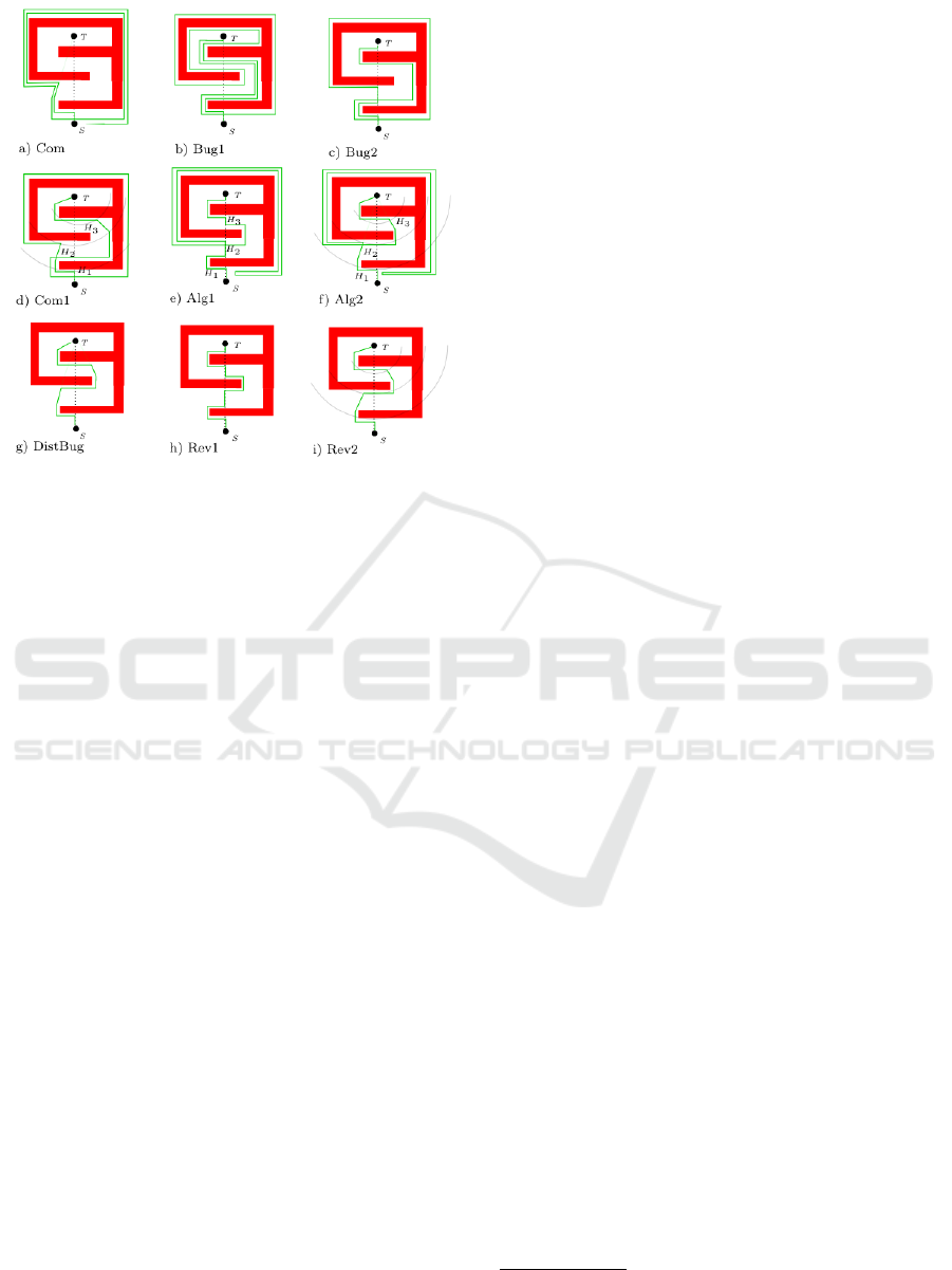
Figure 2: Behaviour of different Bug Algorithms. Here, the

environment conﬁguration is chosen to show typical cases,

in some cases algorithms may be favoured over others or

vice versa. (This Figure is taken from the article (McGuire

et al., 2019)).

points visited previously during the contour of the ob-

stacles. For this, the authors propose an algorithm

based on Bug2 under the name of Alg1. Its principle

is to change the direction of the contour following,

if the mobile encounters a hit-point already visited

(see 2 (e)). The authors also developed another ver-

sion of this algorithm under the name of Alg2. The

idea consists in adding an M-line, which allows in

certain cases to optimize the trajectories (see Figure

2 (f)). Also, in the same article the author proposes a

new version of the Com algorithm named Com1, the

idea consists in memorizing the distance of the last

reference point leave-point compared to the goal (see

Figure 2 (d)).

DistBug is an algorithm described (Kamon and

Rivlin, 1997). It is similar to Alg2 except that it

only keeps in memory the last position of hit-points,

which makes it more efﬁcient at the memory level.

Another aspect that characterizes DistBug is that it

does not impose a direction of bypassing obstacles, it

is always done in the direction of the M-line, as il-

lustrated in Figure 2 (g). In some conﬁgurations this

strategy fails completely.

In the (Horiuchi and Noborio, 2001), authors pro-

pose two algorithms Rev1 and Rev2 (see Figure 2

(h) and (i)). Here, the strategy consists in alternating

the direction at each leave-point to follow a trajectory

that looks like a slalom. The idea behind this strategy

is to change direction if the mobile passes the same

point, which increases the chances of ﬁnding a path.

More recently, (Lentzas and Vrakas, 2020) de-

scribed the LadyBug algorithm. The algorithm uses

a Received Signal Strength Indication (RSSI) of an

electromagnetic signal to detect its position in regard

to signal source. The algorithm is able to accurately

calculate the position of the beacon emitting said sig-

nal. The algorithm is based on two functions: Locali-

sation and Navigation. The algorithm is able to locate

the source of an electromagnetic signal and navigate

to it.

We have described how a few insect-inspired al-

gorithms work, but there are many more. The Bug

Algorithms shown here are generally suitable for en-

vironments such as labyrinths, they are poorly suited

for mobile robots able to see far ahead (without hit-

ting obstacles). Because in an environment where it

is possible to see far ahead, this information can be

used to improve its trajectory. Moreover, these algo-

rithms are not capable of accurately remembering the

places already visited.

3 THE LIMITS OF THESE

ALGORITHMS FOR NAMO

The ﬁrst algorithms described here are based on total

or partial knowledge of the environment to calculate

paths. It is obvious that these techniques cannot be

used if one considers that the environment changing

after moving obstacles as in the NAMO environment.

In addition, these algorithms do not work immedi-

ately, they rely on techniques such as SLAM (Kol-

hatkar and Wagle, 2021) to get the map of the envi-

ronment.

SLAM techniques consist in exploring the envi-

ronment to build a map, then the produced map is

used to calculate an optimal path between two posi-

tions with using path ﬁnding algorithm. In the case

of an environment with a lot of obstacles, generate

a lot of gray areas

, it is obvious that most of the

mapped regions are not used when calculating an op-

timal path between two positions. In fact, this tech-

nique unnecessarily explores certain regions. More-

over, in the case of a dynamic environment, the con-

structed map quickly becomes obsolete, if the obsta-

cles change place. In the context of an environment

with many obstacles, this technique proves to be un-

suitable in the event that certain areas are not accessi-

ble.

In the case of Bug Algorithms, it is true that the

Areas where you have to bypass the obstacle to map

the environment (behind obstacles, places inaccessible by

obstacle avoidance, etc.)

ICAART 2023 - 15th International Conference on Agents and Artiﬁcial Intelligence

214

mobiles are immediately operational and do not re-

quire a preliminary exploration of the environment.

But in certain conﬁgurations of the environment (in

question of the local minima

) these algorithms can

lead to these cycles (go through the same path) be-

cause they do not memorise the conﬁguration of the

environment already explored. In addition, these al-

gorithms do not offer any path improvement in the

case where the mobile has to redo the same path al-

ready taken before. In addition, these algorithms are

not based on metrics or heuristics, which makes it dif-

ﬁcult to use path search algorithms such as D∗ or oth-

ers. The Bug Algorithms try to ﬁnd trajectories in a

straight line towards the objective, but do not memo-

rise the places already explored.

We believe that it is important to propose a plan-

ner for NAMO that beneﬁts from the advantages of

both approaches. Namely, to move directly towards

the objective and rely on the local planner to solve the

obstacles that lie ahead. Otherwise, quickly recalcu-

late a path (as straight as possible towards the goal)

without returning to the areas already explored.

In the next section, we propose an algorithm that

merges the two approaches. It allows the robot to go

straight, in case an obstacle blocks its path, then it cal-

culates a new path (based on a heuristic) that allows

it to move away from the obstacle while approaching

its goal. It also keeps track of the areas visited later

so that it does not have to re-explore in the event that

a path is not found in the direction taken.

4 HEAD-STAR ALGORITHM (H

∗

)

The HeadStar algorithm noted (H

∗

), is halfway be-

tween bug algorithms and heuristic path search algo-

rithms. It uses only a single heuristic

f (x) = h. Like

bug algorithms, H

∗

does not previously have a map of

the environment. To explore its environment, it must

move around. The mobile has a sensor with a cer-

tain range. Like the classic path ﬁnding algorithms,

∗

uses heuristics to optimise navigation paths and

avoid unnecessary explorations. The H

∗

algorithm

uses cell division to represent its environment. The

sensor range is shown with white cells; grey cells

The problem of the local minima occurs when a mobile

navigating without a priori knowledge of the environment is

trapped in a loop. This occurs especially if the environment

consists of concave obstacles, labyrinths, etc. To get out

of the loop, the robot must understand its repeated crossing

through the same environment, which involves memorising

the environment already explored.

Here the heuristic is calculated using Euclidean dis-

tance, other calculation methods are possible such as Man-

hattan distance, Chebyshev distance, etc.

show unexplored areas (see Figure 4), obstacles are

shown with hatched cells. The heuristic is calculated

with respect to the goal cell.

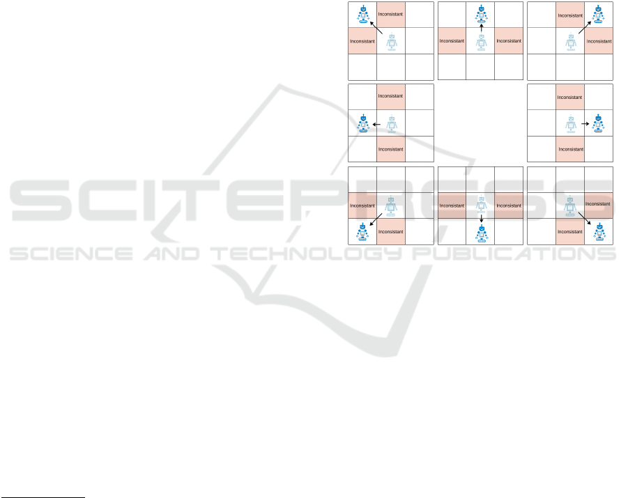
To prevent the algorithm from spreading in width

and to force it to go forward, or to follow the con-

tours, we have introduced the notion of inconsistency.

A cell marked inconsistent will not be explored as

long as there are cells in the open list. The choice

of inconsistent cells is made when moving from one

cell to another. Horizontally and vertically, the mo-

bile marks the cells adjacent to the starting square. In

diagonal displacement, we mark the cells adjacent to

the transition. The different cases are illustrated in

Figure 3.

Figure 3: How to determine inconsistent cells.

∗

uses priority queues to store nodes (cells) to be

visited, and a stack to store nodes already visited. The

priority queues are ordered according to f (x) = h; if

two elements have the same value then we use g as

discriminant f (x) = h + g. h is the estimate of the

distance between this position and the goal, g is the

distance between the mobile and this position. The

different lists used by the algorithm are as follows:

• Open list: priority queue (ordered by h, g + h)

stores newly discovered vertices.

• List inconsistent: priority queue (ordered accord-

ing to h, g + h) stores inconsistent vertices.

• Closed list: a stack which stores the vertices al-

ready visited.

From the starting position, H

∗

inserts the starting

cell in the open list to initiate the process. As long as

the open list and inconsistent list are not empty, we

repeat the following process: We calculate the heuris-

tics of the adjacent cells, and we insert them into the

priority list, open list (if they are not already in one

of the two lists). We remove the ﬁrst element of the

Head Star (H*): A Motion Planning Algorithm for Navigation Among Movable Obstacles

215

open list. If this list is empty, then we remove the

ﬁrst position in the list inconsistent, and we move to

this position if the displacement is direct (only one

cell displacement). If not, we recall the algorithm re-

cursively (the lists are deﬁned in the stack; during the

recursive call, the lists are emptied and ﬁnd their con-

tent when unstacking). During the displacement (in

the case where the displacement is of only one cell),

we insert the visited position in the list closed and we

calculate the inconsistent positions and insert them in

the list inconsistent, each time taking care to remove

the positions in their initial lists. The algorithm ends

if it reaches the goal or after both list open and list

inconsistent are empty. This algorithm is described in

the Algorithm 1.

The function GetNeighbors(s) returns a list of

adjacent cells that are not obstacles. A cell is said

to be adjacent s

if and only if the distance g (distance

between the cells s and s

) is of a single cell: g(s,s

) ≤

√

2 and h(s

) 6= ∞.

The function MinCell(OPEN, INCONS,

goal

) returns the smallest element in the open list.

If the list is empty then it looks for the smallest

elements in inconsistency list.

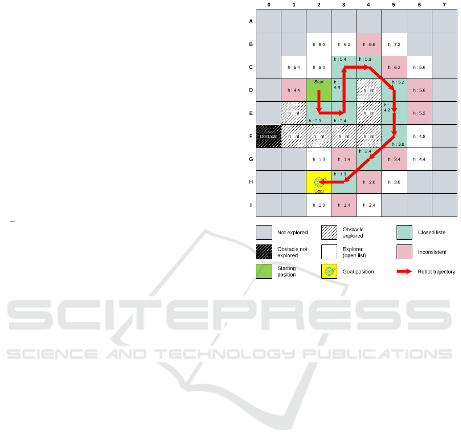
4.1 Illustration of H

∗

Figure 4 shows how H

∗

works. We start by adding

the starting position (D2) in the open list, we calcu-

late the Euclidean distance to the objective on the ad-

jacent cells, we assign an inﬁnite value to the impass-

able cells and we add them to the open list (only cells

with h 6= ∞). We move in the cell with a minimum

h (E2) and note the cells (D1 and D3) as inconsistent

(add these two cells in list inconsistent and remove

them from the open list). When we move into a cell,

we remove it from the two lists (open list and incon-

sistent list) and put it in closed list. The next cell with

h minimum in the open list is (E3), so we move to

this cell directly (in this case the algorithm makes a

recursive call and starts again as the starting position

(E3) and arrival position C3). As long as the open list

is not empty, we continue the same process. If the

open list is empty then we look to see if there are any

elements left in inconsistent list.

5 EXPERIMENTS AND RESULTS

Here, we will compare the H

∗

algorithm to the D

∗

Lite

and A

∗

algorithms. Results are obtained statistically

using 3000 ×26 tests. The number of obstacles starts

at 0 and goes up to 300 obstacles on a surface of 20 ×

20. The number of obstacles is gradually increased in

Figure 4: Sample case.

increments of 10 every 3000 attempts. Beyond 300

obstacles on a surface of 20 ×20, or a density of 0.75,

it becomes difﬁcult to ﬁnd a path between the starting

position and the ﬁnishing position.

We wish to emphasize that H

∗

must move to

explore its environment, unlike the algorithms with

which we compared it. To make a fair comparison,

we have assigned tests assuming that D

∗

Lite has no

prior knowledge of its environment. Technically, this

operation is carried out by generating the obstacles af-

ter the ComputePath() function. Figure 6 (A) graph

shows equivalent performance—in terms of distance

traveled— (slightly in favor of H

∗

). But D

∗

Lite is not

able to work in an environment where the goal is not

known in advance or where the goal is moving. This

explains why H

∗

travels a greater distance.

The graph in Figure 6 (B) shows a comparison of

the three algorithms in terms of distance, execution

time and nodes in open list. We notice that D

∗

Lite is

time consuming when the number of obstacles is low.

This is due to the fact that many nodes are found in the

open list (as we can see in 6 (C)), and the key calcu-

lation is based on two criteria (in the implementation

used here, the open list is implemented in a dictio-

nary, the key being a pair of integers indicating the

abscissa and the ordinate of the cell. The value is

composed of a pair of doubles <min(g(s),rhs(s)) +

h(s

start

,s),min(g(s),rhs(s)) >. The process of get-

ICAART 2023 - 15th International Conference on Agents and Artiﬁcial Intelligence

216

Algorithm 1: Algorithme HeadStar.

1: function COMPUTEPATH(S

start

goal

,Path)

2: OPEN ←

3: INCONS ←

4: CLOSE ←

5: s ← S

start

6: OPEN.insert(s)

7: while OPEN.size() /∈

0 or INCONS.size() /∈

0 do

8: ADDTOCLOSELIST(s,OPEN,INCONS,CLOSE)

9: Path.insert(s)

10: if s = S

goal

then

11: return True  Path found

12: end if

13: for all s

∈GETNEIGHBORS(s) do

14: ADDTOOPENLIST(s,OPEN, INCONS,CLOSE)

15: end for

16: next

pos ← MINCELL(OPEN, INCONS, S

goal

)

17: if next pos =

0 then

18: return False  No path available

19: end if

20: if |next pos −s|≤

√

2 then

21: inc list ←GETINCONSISTANT(s,next pos)

22: for each s

∈ inc list do

23: ADDTOINCONSISTANTLIST(s, OPEN,INCONS,CLOSE)

24: end for

25: s ← next pos

26: else

27: if COMPUTEPATH(s,next pos, Path) then

28: s ← next pos

29: end if

30: end if

31: end while

32: return

33: end function

ting the minimum cell in the open list is implemented

in the TopKey(open list) function, using the sort

function of the STL (see Listing 1)). The two remain-

ing algorithms, occupy linear time although H

∗

is a

little more efﬁcient than A

∗

. Again, this is due to the

number of nodes found in open list; it is larger in A

∗

b o o l

comp are ( p a i r <p a i r <i n t , i n t > ,

p a i r <do uble , doub le>> x ,

p a i r <p a i r <i n t , i n t > ,

p a i r <do uble , doub le>> y ){

r e t u r n (

x . s ec o nd . f i r s t <= x . s e c o n d . f i r s t &&

y . s ec o nd . se c on d <= y . s ec o nd . se c on d

) ;

}

p a i r <do uble , dou ble>

D L i g h t S t a r : : TopKey ( o p l s t &l s o p e n ) {

l s o p e n . s o r t ( co mpa re ) ;

r e t u r n l s o p e n . f r o n t ( ) . se c o n d ;

}

Listing 1: Cell with the lowest key.

Image 5 shows the use of H

∗

with the robot Turtle-

Bot3 in the Gazebo simulator and RViz. Image (A)

shows the environment of the robot in the Gazebo

simulator. The robot’s start position and the goal po-

sition are shown with red circles. The robot maps

its environment using a LIDAR. The ﬁgures from (1)

to (8) are generated by RViz; they show the different

stages through which the robot goes to reach its objec-

tive. The areas in dark grey show unrecognised areas

and, in light grey the free spaces. Obstacles are repre-

sented by black areas. The robot’s position is always

indicated with the red circle. Figure (B) shows the

Robot’s trajectory from its starting position to its goal

Head Star (H*): A Motion Planning Algorithm for Navigation Among Movable Obstacles

217

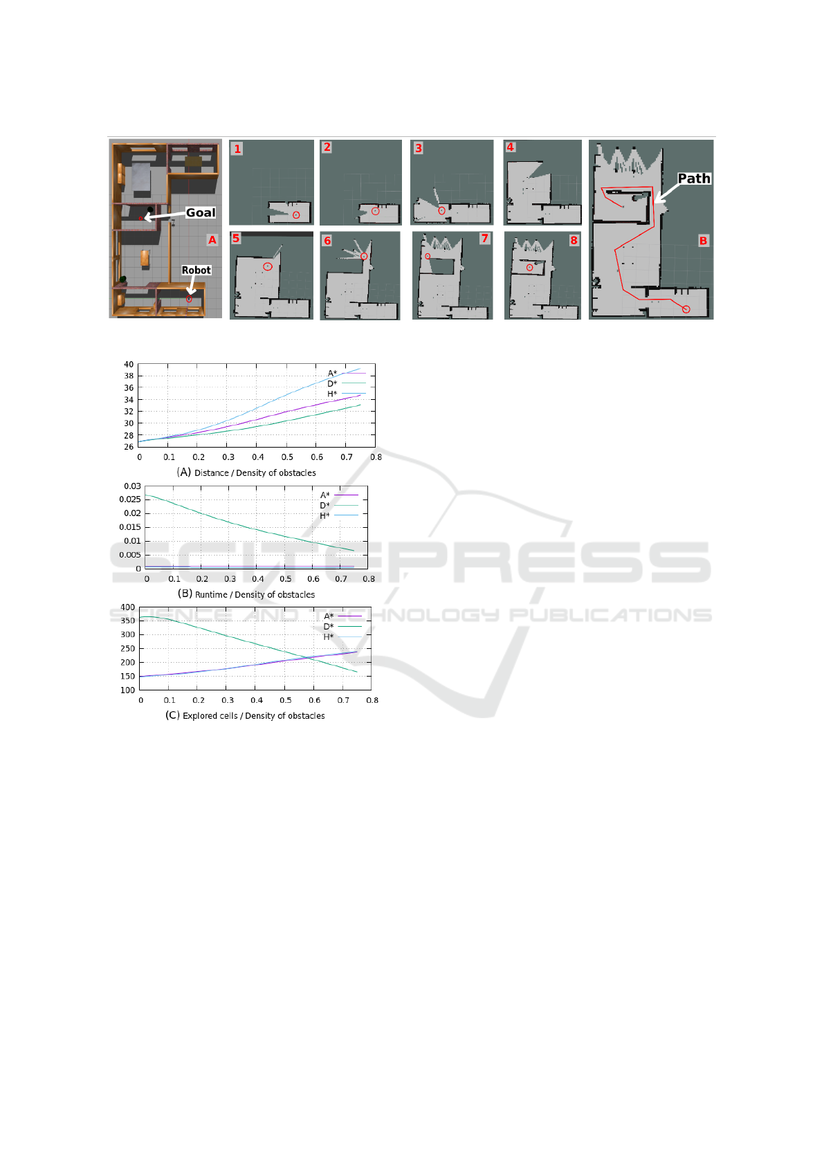
Figure 5: Simulation of H

∗

with the TurtleBot 3 robot in Gazebo.

Figure 6: Comparison of H

∗

with A

∗

and D

∗

Lite algo-

rithms.

position.

6 CONCLUSIONS

In this article, we have presented H

∗

, a motion plan-

ning algorithm for NAMO. The principle is to com-

bine the techniques of bug algorithms and path search

algorithms which use heuristics. The ﬁrst results ob-

tained in simulation are very interesting, they show

that H

∗

is able to ﬁnd a path without providing it with

a map beforehand. In our experiments, we noticed

that H

∗

provides a path equivalent to D

∗

Lite in most

typical environment conﬁgurations. Among the pos-

sible improvements that we are experimenting with

is that of ﬁnding the best way to determine inconsis-

tent cells in order to improve the performance of H

∗

in terms of distance traveled. We have also started to

experiment with our algorithm on a mobile robot in a

real environment.

REFERENCES

Charalampous, K., Kostavelis, I., and Gasteratos, A. (2017).

Recent trends in social aware robot navigation: A sur-

vey. Robotics and Autonomous Systems, 93:85–104.

Chen, G., Luo, N., Liu, D., Zhao, Z., and Liang, C.

(2021). Path planning for manipulators based on an

improved probabilistic roadmap method. Robotics

and Computer-Integrated Manufacturing, 72:102196.

Eiben, E. and Kanj, I. (2017). How to navigate through

obstacles? arXiv preprint arXiv:1712.04043.

Horiuchi, Y. and Noborio, H. (2001). Evaluation of path

length made in sensor-based path-planning with the

alternative following. In Proceedings 2001 ICRA.

IEEE International Conference on Robotics and Au-

tomation (Cat. No. 01CH37164), volume 2, pages

1728–1735. IEEE.

Kalpitha, N., Murali, S., et al. (2020). Optimal path plan-

ning using rrt for dynamic obstacles. Journal of Scien-

tiﬁc and Industrial Research (JSIR), 79(06):513–516.

Kamon, I. and Rivlin, E. (1997). Sensory-based motion

planning with global proofs. IEEE transactions on

Robotics and Automation, 13(6):814–822.

Koenig, S. and Likhachev, M. (2002). Dˆ* lite. Aaai/iaai,

15.

Kolhatkar, C. and Wagle, K. (2021). Review of slam al-

gorithms for indoor mobile robot with lidar and rgb-

d camera technology. Innovations in Electrical and

Electronic Engineering, pages 397–409.

LaValle, S. M. (2006). Planning algorithms. Cambridge

university press.

LaValle, S. M. et al. (1998). Rapidly-exploring random

trees: A new tool for path planning.

ICAART 2023 - 15th International Conference on Agents and Artiﬁcial Intelligence

218

Lentzas, A. and Vrakas, D. (2020). Ladybug. an inten-

sity based localization bug algorithm. In 2020 25th

IEEE International Conference on Emerging Tech-

nologies and Factory Automation (ETFA), volume 1,

pages 682–689. IEEE.

Lumelsky, V. and Stepanov, A. (1986). Dynamic path plan-

ning for a mobile automaton with limited information

on the environment. IEEE transactions on Automatic

control, 31(11):1058–1063.

McGuire, K. N., de Croon, G. C., and Tuyls, K. (2019). A

comparative study of bug algorithms for robot naviga-

tion. Robotics and Autonomous Systems, 121:103261.

Moghaddam, S. K. and Masehian, E. (2016). Planning robot

navigation among movable obstacles (namo) through

a recursive approach. Journal of Intelligent & Robotic

Systems, 83(3):603–634.

Renault, B., Saraydaryan, J., and Simonin, O. (2019). To-

wards s-namo: socially-aware navigation among mov-

able obstacles. In Robot World Cup, pages 241–254.

Springer.

Sankaranarayanan, A. and Vidyasagar, M. (1990). A new

path planning algorithm for moving a point object

amidst unknown obstacles in a plane. In Proceedings.,

IEEE International Conference on Robotics and Au-

tomation, pages 1930–1936. IEEE.

Sivaranjani, S., Nandesh, D. A., Gayathri, K., Ramanathan,

R., et al. (2021). An investigation of bug algorithms

for mobile robot navigation and obstacle avoidance

in two-dimensional unknown static environments. In

2021 International Conference on Communication

information and Computing Technology (ICCICT),

pages 1–6. IEEE.

Stilman, M. and Kuffner, J. J. (2005). Navigation among

movable obstacles: Real-time reasoning in complex

environments. International Journal of Humanoid

Robotics, 2(04):479–503.

Head Star (H*): A Motion Planning Algorithm for Navigation Among Movable Obstacles

219