Co-Incrementation: Combining Co-Training and Incremental Learning

for Subject-Speciﬁc Facial Expression Recognition

Jordan Gonzalez

, Thibault Geoffroy

, Aurelia Deshayes

and Lionel Prevost

Learning, Data and Robotics (LDR) Lab, ESIEA, Paris, France

Laboratoire d’Analyse et Math

ematiques Appliqu

ees (LAMA), UPEC, Cr

eteil, France

Keywords:

Incremental Learning, Semi-Supervised Learning, Co-Training, Random Forest, Emotion Recognition.

Abstract:

In this work, we propose to adapt a generic emotion recognizer to a set of individuals in order to improve

its accuracy. As this adaptation is weakly supervised, we propose a hybrid framework, the so-called co-

incremental learning that combines semi-supervised co-training and incremental learning. The classiﬁer we

use is a speciﬁc random forest whose internal nodes are nearest class mean classiﬁers. It has the ability to learn

incrementally data covariate shift. We use it in a co-training process by combining multiple view of the data

to handle unlabeled data and iteratively learn the model. We performed several personalization and provided a

comparative study between these models and their inﬂuence on the co-incrementation process. Finally, an in-

depth study of the behavior of the models before, during and after the co-incrementation process was carried

out. The results, presented on a benchmark dataset, show this hybrid process increases the robustness of the

model, with only a few labeled data.

1 INTRODUCTION

These last decades, the ﬁeld of automated emotion

recognition has dramatically grown. New solutions,

mainly based on machine learning algorithms, have

been developed. New data sets have been shared

within the research community and many emerging

applications are starting to mature in various ﬁelds

like video gaming, education, health, medical diagno-

sis, etc. Nevertheless, many challenges remain, like

face lightning or face pose (Sariyanidi et al., 2014).

In this paper, we address the challenge of identity

bias. The individual variability between people has

a direct consequence on the recognition of emotions

(Senechal et al., 2010). On the morphological level,

the shape and ”texture” (skin, wrinkles) of the face

differ according to different factors (gender, age, etc.).

On the behavioral level, each subject has his own way

of expressing emotion, depending on his introverted

or extroverted personality.

It is well known that building accurate classiﬁers

involves gathering labeled data. Due to time and cost

constraints, it seems irrational to expect labeling hun-

dreds or even thousands of data that would be nec-

essary to train today’s models in a supervised way.

Moreover, labeling (potentially many) new affective

data corresponding to new subjects seems too costly.

To solve this issue, one solution is to personal-

ize generic classiﬁers. In detail, these classiﬁers are

trained on large-scale datasets containing many sub-

jects. Obviously, regardless of the dataset size, it is

highly unlikely to capture all of the inter-subject vari-

ability in terms of morphology and behavior. Con-

sequently, these generic “omni-subjects” classiﬁers

will perform the best they can, given the biases de-

scribed above. The idea behind personalization is

to adapt these classiﬁers to a given set of subjects

(multi-subjects approach), or even to one particular

subject (mono-subject approach). Researchers in ar-

eas like handwriting recognition (Oudot et al., 2004)

and speech recognition (Meng et al., 2019) got to

work on this ”variability problem”. To overcome this

challenge, they built self-adaptation (incremental) al-

gorithms. The general idea of these algorithms is

to continuously adapt a generic (”world”) model to

personalize it on one single user, by using language

constraints, for example. Unfortunately, for emotion

recognition in images, such rules do not exist. That is

why we need to turn to other solutions.

In the ﬁeld of semi-supervised learning, the co-

training algorithm (detailed in the next section) uses

several models, trained on labeled data, to predict

the class (also called pseudo-label) of unlabeled data.

Then, it add these data to labeled set and retrain the

models on this augmented dataset. This process has a

high cost in terms of computational time.

270

Gonzalez, J., Geoffroy, T., Deshayes, A. and Prevost, L.

Co-Incrementation: Combining Co-Training and Incremental Learning for Subject-Speciﬁc Facial Expression Recognition.

DOI: 10.5220/0011635200003411

In Proceedings of the 12th International Conference on Pattern Recognition Applications and Methods (ICPRAM 2023), pages 270-280

ISBN: 978-989-758-626-2; ISSN: 2184-4313

 2023 by SCITEPRESS – Science and Technology Publications, Lda. Under CC license (CC BY-NC-ND 4.0)

The main proposal of this work is to combine co-

training with incremental learning in order to avoid

this issue. Initial models are generic ones, trained on

a large set of subjects. They are used to predict the

pseudo-label of new data, corresponding to new sub-

jects. After pseudo-labeling these new samples, we

apply incremental learning technics to adapt the mod-

els. Therefore, these models are no more generic, but

personalized to new subjects. We called this process

co-incrementation learning. One of its main advan-

tage is to reduce drastically the computing time while

improving the recognition accuracy on new subjects,

thus reducing the identity bias.

The rest of the article is as follows. Next section

will present the incremental learning ﬁeld with a par-

ticular focus on random forest (RF)-based algorithms

and detail the co-training process. Section 3 is de-

voted to the data and the feature extraction process.

Section 4 presents in detail the nearest-class mean for-

est (NCMF), how it differs from classical RF and the

way it can learn incrementally. In section 5, we detail

the original co-incrementation algorithm that com-

bines incremental NCMF with co-training. Then, we

present in section 6 results obtained on generic mod-

els (before adaptation) and after co-incrementation on

speciﬁc chunks. Finally, we conclude in section 7.

2 RELATED WORKS

Automatic Facial Emotion Recognition (FER) has re-

ceived wide interest in a variety of contexts, espe-

cially for the recognition of action units, basic (or

compound) emotions and affective states. Although

considerable effort has been made, several questions

remain about which cues are important for interpret-

ing facial expressions and how to encode them. Af-

fect recognition systems most often aim to recognize

the appearance of facial actions, or the emotions con-

veyed by those actions (Sariyanidi et al., 2014). The

former are generally based on the Facial Action Cod-

ing System (FACS)(Ekman, 1997). The production

of a facial action unit has a temporal evolution, which

is typically modeled by four temporal segments: neu-

tral, onset, apex, and offset (Ekman, 1997). Among

them, the neutral is the phase with no expression and

no sign of muscle activity; the apex is a plateau where

the maximum intensity usually reaches a stable level.

As seen before, identity bias results in perfor-

mance losses on generic learning models. Strategies

for grouping individuals by common traits such as

gender, weight, or age and personalizing models on

these groups have already shown promising results

in a wide range of areas such as activity recognition

(Chu et al., 2013) (Kollia, 2016) (Yang and Bhanu,

2011). However, quite often the strategy used con-

sists in personalizing one model per user since it en-

sures better results. This can quickly become complex

when the number of subjects increases or when the

number of collected data per subjects keeps small. In

the ﬁeld of emotion recognition, different solutions to

this challenge have been considered, personalization

methods being the most promising (Chu et al., 2013)

(Yang and Bhanu, 2011).

One of the main characteristics of incremental

techniques is the ability to update models using only

recent data. This is often the only practical solution

when it comes to learning data ”on the ﬂy” as it would

be impossible to keep in memory and re-learn from

scratch every time new information becomes avail-

able. This type of technique holds promise for per-

sonalizing models to individuals. It has been demon-

strated that Random forests (RF) (Breiman, 2001), in

addition to their multi-class nature and ability to gen-

eralize, have also the ability to increment in data and

classes (Denil et al., 2013) (Hu et al., 2018) (Lak-

shminarayanan et al., 2014) . Besides, Random for-

est models have been used successfully for personal-

ization (Chu et al., 2013) (Kollia, 2016) (Yang and

Bhanu, 2011). Nearest class mean forests derived

from RF, have demonstrated to be able to outperform

RF performance and allow an easy way to perform in-

crementation (Ristin et al., 2014), even in the emotion

recognition ﬁeld (Gonzalez and Prevost, 2021).

In the era of big data, with the increase in the

size of databases, the ﬁeld of machine learning faces

a challenge, the creation of ground truth, which can

be costly in time and effort. We are therefore in-

creasingly ﬁnding ourselves in contexts of incom-

plete supervision, where we are given a small amount

of labeled data, which is insufﬁcient to train a good

learner, while unlabeled data is available in abun-

dance. To this end, different learning techniques have

been proposed (Zhou, 2018) with human intervention

such as active learning (Settles, 2009) or without hu-

man intervention such as semi-supervised methods.

One of these last ones is based on disagreement meth-

ods (Zhou and Li, 2010), co-training being one of its

most famous representations.

Co-training is a learning technique proposed in

1998 by Blum and Mitchell (Blum and Mitchell,

1998) which is traditionally based on the use of two

machine learning models. The main idea is that they

complement each other: one helps the other to cor-

rect the mistakes it does not make, and vice versa.

A second idea is to exploit data that are not labeled

(present in large quantities), rather than processing

only labeled data (present in small quantities). For

Co-Incrementation: Combining Co-Training and Incremental Learning for Subject-Speciﬁc Facial Expression Recognition

271

this to work, the dataset must be described according

to two independent views, i.e., two different represen-

tation spaces for this same dataset. Otherwise, their

potential to provide each other with relevant informa-

tion is limited. Although, this assumption is difﬁcult

to achieve in practice, as Wang and Zhou explain in

2010 in their study on co-training (Wang and Zhou,

2010).

During co-training, estimations of probabilities

are mainly needed (see Sec.5.1) and act as conﬁdence

levels. For a decision tree (DT), this is deduced from

the statistics stored in the leaves during the learning

process. Unfortunately, DTs are considered as poor

estimators of these probabilities and suggestions have

been made to compute the posterior probabilities dif-

ferently, one of them being to apply a Laplace cor-

rection (Provost and Domingos, 2003)(Tanha et al.,

2017). Semi-supervised learning was ﬁrst proposed

in 2003 to effectively use unlabeled data for facial

expression recognition with the Cohn-Kanade dataset

(Cohen et al., 2003). It consists in switching models

during co-training when performance collapses. In-

deed, one of the drawbacks of co-training is the label-

ing error that can occur during co-training iterations.

This effect can then be tackled either by placing less

conﬁdence in the model, by setting a higher threshold,

or by looking for strategies to correct these errors on

the ﬂy (Zhang et al., 2016).

An observable limitation in the co-training pro-

cedure is that the classiﬁer retains multiple training

sessions on the same set of data. We could take ad-

vantage of the progress in incremental learning to

make only one pass and update the tree while pseudo-

labeling the data without re-training from scratch at

each iteration.

3 DATASETS AND FEATURE

EXTRACTION

3.1 Datasets

3.1.1 Compound Facial Expressions of Emotion

(CFEE)

The CFEE dataset contains 230 subjects with one im-

age for each of the 22 categories present in the dataset:

6 basic emotions (anger, surprise, sad, happy, fear,

disgust), 15 compound emotions (i.e. a combination

of two basic emotions), and the neutral expression

(Du et al., 2014). For each subject, we selected 7

images with the six basic emotions and the neutral

face (the dataset doesn’t have the contempt emotion).

Thus, 1285 images are retained to train the NCMF

baseline classiﬁer and 322 for evaluation.

3.1.2 Extended Cohn-Kanade CK+

The CK+ dataset is the most popular database in the

ﬁeld of emotion recognition. It contains 327 labeled

sequences of deliberate and spontaneous facial ex-

pressions from 123 subjects, 85 females and 38 males

(Lucey et al., 2010). A sequence lasts approximately

20 frames in average (from 4 to about 60), and always

begins with a neutral expression, then progresses to

a speciﬁc expression until a peak in intensity (apex)

that is labeled using the Facial Action Coding Sys-

tem (FACS) (Ekman, 1997). By collecting the labeled

images (without including the emotion of contempt),

and by focusing on neutrals and apexes we collect

1802 images labeled among the 6 basic emotions (590

for men, and 1202 for women).

3.2 Feature Extraction

The OpenFace library developed by (Baltru

saitis

et al., 2016) was used to extract 68 facial land-

marks and high level features, namely, facial Action

Units (AUs). We then extracted Local Binary Pat-

terns (LBP) and Histograms of oriented Gradients

(HoG) features with the scikit-image library from the

cropped faces registered by OpenFace.

4 NEAREST CLASS MEAN

FOREST

4.1 Original Algorithm

Nearest Class Mean Forest (NCMF) (Ristin et al.,

2014) is a Random Forest (RF) (Breiman, 2001)

whose nodes are Nearest Class Mean (NCM) (Hastie

et al., 2009) classiﬁers. In these nodes, two class cen-

troids (called c

and c

) are computed. They are used

to direct samples x (given a distance measure) to the

left child of the node (if x is closer to c

than c

) or its

right child (otherwise). A class bagging occurs during

training: only a random subset of available classes is

considered in each node. The splitting decision func-

tion is also modiﬁed. Among the data available in the

current node n, we can compute all the possible pairs

of centroids. The optimal pair is the one that maxi-

mizes the Information Gain I (Quinlan, 1986).

The main advantage of NCM forests is their abil-

ity to learn new data and classes incrementally. Two

incremental strategies, namely, Update Leaf Statis-

tics (ULS) and Incremental Growing Tree (IGT) have

ICPRAM 2023 - 12th International Conference on Pattern Recognition Applications and Methods

272

been introduced in (Ristin et al., 2014). The incre-

mental data is propagated, as in a prediction phase,

in each tree of the forest; then, the occurrences at

the level of the predicting leaves are updated (ULS).

Since the ULS strategy only updates the distributions

in the leaves of the tree, when incremental data ap-

pear, the distributions evolve and thus the predictions

are likely to change. With the IGT strategy, we ﬁrst

proceed as with ULS; then, right after the update of

the class distributions of the leaf, we check if the in-

crement satisﬁes a condition that could locally lead to

the construction of a subtree, e.g. majority label mod-

iﬁcation. If this is the case, the leaf is transformed

into a node, which triggers the recursive construction

of the subtree from this position. The data consid-

ered by the subtree are all those that were present in

this leaf, either during the learning or during the in-

crementation.

4.2 Probabilistic Decision Criterion

Classically, for decision trees, a test sample is propa-

gated from the root node to a terminal leaf. Then, the

decision is made by the majority class present in this

leaf. For tree forests, a majority vote is applied on tree

decisions.

As explained above, co-training needs to evaluate

the conﬁdence we have in each view for a given sam-

ple. So, we need to compute a posterior probability

vector. Then, using the maximum a posteriori rule,

we take the highest probability and use a conﬁdence

threshold to decide whether x will be used for incre-

mental training or not.

Given a sample x, let φ

: R

7→ R

be the predic-

tion function associated with the model µ and return-

ing a vector containing the class conditional posterior

probabilities:

∀x ∈ R

, φ

(x) = [P(k

|x), ..., P(k

|x)], (1)

where

• K = {k

, ..., k

} is the set of l labels,

• x is an observation to be classiﬁed,

• P(k

|x) the conditional (posterior) probability that

x belongs to the class k

, for 1 ≤ i ≤ l.

The class assigned to the observation x, l

(x), is

then determined by the rule of the maximum a poste-

riori:

(x) = argmax

∈K

[P(k

|x), ..., P(k

|x)]. (2)

We establish a conﬁdence criterion, consisting in

attributing a threshold θ such that:

max[P(k

|x), ..., P(k

|x)] ≥ θ. (3)

If the forest is composed of t trees, we have t pre-

diction vectors for a test sample. It is thus necessary

to deﬁne an operator to combine optimally these vec-

tors.

Consider, for an observation x and a decision

tree t, the vector S

(x) = [S

|x), ..., S

|x)], where

|x) corresponds to the number of occurrences of

the class k

in each leaf of t. The vector φ

is then

computed as follows:

(x) =

R(x)

∑

t∈T

(x). (4)

with,

R(x) =

∑

t∈T

∑

i=1

|x). (5)

We ﬁrst aggregate the values of all the predictor

leaves and then, calculate the global probability at the

forest level (4). Thus, a leaf with a smaller number of

class members than another leaf will have less impact

in the ﬁnal calculation of the φ

(x) probabilities.

5 CO-INCREMENTATION

ALGORITHM

5.1 Original Co-Training Algorithm

Co-training (Blum and Mitchell, 1998) is a semi-

supervised learning technique that can be used

when a dataset is partially labeled. It involves the

collaboration between two machine learning models.

Let V

and V

be two families of features, also

called ”views”, fully describing each observation of

the dataset x = (V

(x),V

(x)). The corresponding

datasets are denoted L

]

, L

]

for labeled data

and U

]

for unlabeled data. Each model is

trained on a view and both models must satisfy the

independence assumption.

1. Pre-Training: each model initially trains on

its own set labeled L

]

or L

]

Co-training is an iterative process. For each ob-

servation of U, the following 2 steps are performed:

2. Labeled Set Extension: each model predicts a

pseudo-label for the observation; the most reliable

prediction (given a conﬁdence criterion) is used to

add the observation and its most reliable pseudo-

label to the labeled set of the other view, L

]

model 1 was the most reliable and vice versa ;

3. Self-Training: the model whose pseudo-label was

the least reliable is re-trained on the new labeled

set.

Co-Incrementation: Combining Co-Training and Incremental Learning for Subject-Speciﬁc Facial Expression Recognition

273

We can notice that single-view classiﬁers require

a complete re-learning at each iteration. This pro-

cess can become expensive in terms of computational

time, especially if the size of U is large.

5.2 Incremental Co-Training Algorithm

(EBSICO)

In this research work, we propose a co-training

method that differs from the classical method (see

Sec.5.1) by using a hybrid method, combining

semi-supervised learning and incremental learning

paradigms. Our aim is not to build generic classi-

ﬁers but to personalize generic classiﬁers to a sub-

set of subjects. Thus, we use a ﬁrst dataset G to

build these generic single-view classiﬁers. Then, the

second dataset I is used to personalize these classi-

ﬁers incrementally by using a co-training based al-

gorithm. The main advantage of this process is to

avoid re-training from scratch the single-view classi-

ﬁers through co-training iterations. Fig. 1 shows the

different steps of our method that are described be-

low:

1. Pre-Training: At step 1, generic single-view clas-

siﬁers are trained respectively on their own views

]

and G

]

. These are the reference models,

and will be referred to by the name of their view.

2. Error-Based Self-Incrementation (EBSI): At

step 2, the model associated to the view V

pre-

dicts a class for each of the observations of L

]

If this predicted class is different from the ground

truth (the dataset L

]

is labeled), the model incre-

ments on this example, with a INCR() function.

This error-based incremental strategy is possible

since we work on generic models that are already

trained. This step is described in the algorithm 1.

3. Error-Based CO-incrementation (EBCO): For

each unlabeled x observation of U

]

(A) We identify the most reliable model, using the

posterior probabilities p

(x) and p

(x):

(x) = max φ

(x). (6)

(x) = max φ

(x). (7)

The largest posterior probability thus informs

us about the most reliable model for predicting

the pseudo-label of x. We use the predictions of

the models l

(x) and l

(x) (see Eq.2) as the

pseudo-label.

(B) Then, the less reliable model is incremented

in a supervised manner from the unlabeled ob-

servation using the pseudo-label provided by

the more reliable model. The algorithm 2 de-

scribes more precisely the co-incrementation

procedure.

Contrary to the classical co-training algorithm,

with our approach EBCO, for each iteration, when

the maximum probability of belonging to a class ex-

ceeds the conﬁdence threshold EBCO, the least reli-

able model does not restart its learning from the be-

ginning. It only increments on the observation of the

considered iteration. Moreover, it increments only if

its pseudo-label differs from the one delivered by the

most reliable model.

Algorithm 1: Error-based Self-incrementation (EBSI).

Require: generic model µ

pretrained on G

]

for all (x, y) ∈ L

]

The model uses the function φ(x) to obtain the

probability vector of class membership:

(i)

← φ(x

]

)

The predicted label is thereby determined as:

← argmax(p

(i)

)

if l

̸= y then

← INCR(µ

, x, y)

end if

end for

Algorithm 2: Error-Based Co-Incrementation (EBCO).

Require: models µ

and µ

incremented following

EBSI method, θ ≥ 0

for all u ∈ U do

Each model uses the function φ

(u) to obtain the

probability vectors of class membership:

(1)

← φ

[V1]

)

(2)

← φ

[V2]

)

The pseudo-labels are then:

← argmax(p

(1)

)

← argmax(p

(2)

)

The probabilities associated are then:

← max(p

(1)

)

← max(p

(2)

)

if p

> p

and p

≥ θ then

if l

̸= l

then

← INCR(µ

, u

[V2]

, l

)

end if

else if p

> p

and p

≥ θ then

if l

̸= l

then

← INCR(µ

, u

[V1]

, l

)

end if

end for

ICPRAM 2023 - 12th International Conference on Pattern Recognition Applications and Methods

274

Figure 1: Diagram describing the entire proposed EBSICO

process - (1): pre-training on the ﬁrst dataset, (2): incre-

menting on labeled samples from the second dataset (EBSI),

(3) incrementing on unlabeled samples from the second

dataset (EBCO), using for each sample the prediction of the

most reliable model as a pseudo-label (A) and increment-

ing the least reliable model with this pseudo labeled sample

(B).

6 EXPERIMENTAL PIPELINE

AND RESULTS

6.1 Data Preparation

To carry out our experiments, in a ﬁrst stage we per-

formed data partitioning. The CFEE dataset is used

to train the generic single view classiﬁers. Thus, it

corresponds to the dataset G. The CK+ database was

divided into two subsets named I and E, used respec-

tively for incremental learning and evaluation. Next,

we split I into L and U subsets corresponding to the

labeled and unlabeled sets, such that L ∪U = I. For

each sequence of n images (e.g. see Figure 2), we

noted i

and i

the ﬁrst and second image correspond-

ing to the neutral emotion and i

n−1

and i

the two last

images of the sequence, corresponding to the maxi-

mum intensity emotion (apex). We aim to evaluate

the ability of co-incrementation to recognize forced

expression after learning subtle ones. For this pur-

pose, the images were assigned to the subsets E and I

as follows:

• E contains the set of images i

and i

• I contains the set of images i

and i

n−1

6.2 Reference Model Training

As described in section 3.2, we extracted low-level

texture features and high-level facial Action Units.

So, each sample x is described by two views: x =

Figure 2: Example of a video sequence from CK+ for the

surprise.

(AU,T X) where AU corresponds to the Action Units

vector and T X to the concatenation of LBP and HoG

vectors.

The NCMFs models were ﬁrst trained in a super-

vised manner on fully labeled CFEE using AU and

T X views. These models, corresponding to step 1 of

the EBSICO procedure, are generic ones. They will

be used as reference models regardless of the person-

alization strategy. For each clustering criterion, we

refer to these models respectively by the names AU

[Θ]

and T X

[Θ]

(see below).

6.3 Personalization Chunking

The purpose of the second stage is to apply data per-

sonalization, which consists in performing data clus-

tering. We are going to separate the data into slots

by grouping them, according to a criterion called per-

sonalization. For each of these criteria where Θ is

the acronym of personalization, we name these mod-

els respectively by AU

[Θ]

and T X

[Θ]

. The proposed

customizations are as follow:

ALL: No customization is an approach that serves

as a baseline and consists of applying the co-

incrementation algorithm directly on all the data

in I, as one would do for a generic model. It uses

only one group containing all the observations of

I. In the following, we refer to this strategy as

ALL.

GENDER: The gender personalization approach

performs a clustering of the data according to the

perceived gender. We obtain two groups of data

named M (man) and W (woman) corresponding

to men and women data respectively. The gender

information has been assigned manually. In the

following, we refer to this strategy as GENDER.

MORPHO: The morphological personalization ap-

proach performs a clustering of the data accord-

ing to the face morphology. To do so, we used

the landmarks (see Sec.3.2) detected on the neu-

tral face of each subject. Then, the K-means al-

gorithm was used on these data to identify several

clusters based on morphological features.

Co-Incrementation: Combining Co-Training and Incremental Learning for Subject-Speciﬁc Facial Expression Recognition

275

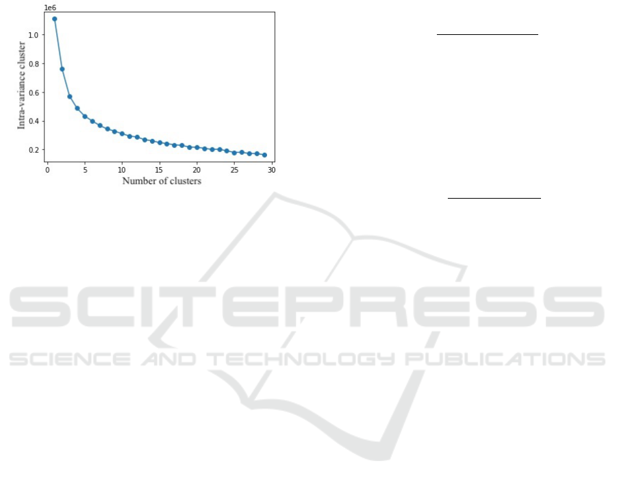
We decided to divide the subjects of the dataset

into 8 slots which we considered as a good com-

promise in terms of number of images per slot and

number of models; ﬁgure 3 illustrates the varia-

tion of the total intra-class variance for a number

k of clusters and conﬁrms us in this choice. In the

following, we refer to this strategy as M ORPHO.

Figure 3: Evolution of the intra-class variance according to

the number of clusters (elbow plot).

Note that each group (cluster) is said to be subject-

independent. On the one hand, these data have not

been seen during the training of the generic models.

On the other hand, all images of the same subject be-

long to the same cluster and the same cluster can con-

tain data of several subjects. For a given cluster, the

associated sets I and E contain the same individuals

but different images (in terms of emotional intensity),

in order to evaluate the impact of personalization on

the reference models after co-incrementation.

6.4 Chunk Specialization

In the third stage of the proposed pipeline, the EB-

SICO process is executed within each chunk as fol-

lows. In our experiments we considered a θ value

of 0.8 and used NCM forests of 50 trees with the

IGT strategy as the incrementation INCR() function

(Ristin et al., 2014).

We decide to use a ratio of 5% of labeled data, so,

in the following, |L| = 0, 05 ∗ |I| and |U| = 0, 95 ∗ |I|.

Then, we execute sequentially and for each single-

view classiﬁers:

• EBSI on L

• EBCO on U

6.5 Model Evaluation per Chunk

The last step of the pipeline consists in evaluating

each model per chunk at different stages of the EB-

SICO procedure, in order to follow its evolution in

terms of personalization. Thus, per view, and per

chunk, we obtain a performance score that we mea-

sure when the model is in the baseline state, at the end

of the EBSI procedure, and at the end of the EBCO

procedure.

To carry out our experiments, we used the accu-

racy metric to evaluate the model performance indi-

vidually:

acc =

∑

x∈X

I(y = l

(x))

|Y |

(8)

where y is the class (ground-truth) of x, the expres-

sion

∑

x∈X

I(y = l

(x)) corresponds to the number of

correct predictions and |Y | to the total number of ob-

servations to be labeled.

Likewise, to evaluate the contribution of a speciﬁc

personalization criterion Θ which may contain several

chunks, we used:

acc

[Θ]

∑

c∈C

acc(c) × |c|

|C|

(9)

where C represents the set of chunks and c corre-

sponds to the samples belonging to a chunk.

6.6 Experimental Results

6.6.1 Impact of Co-Incrementation

The purpose of this analysis is to evaluate the con-

tribution provided by the whole co-incrementation

process (EBSICO). Tables 1 and 2 describe the

results obtained for the single-view models trained

respectively on the AU and T X views. The ﬁrst

column reports the baseline accuracy (before co-

incrementation). The second and third columns re-

port the accuracy after applying sequentially EBSI

and EBCO processes.

We can observe that for low labeling rates, the

EBSI process does not inﬂuence and in some cases

decreased the prediction performance. Thus, per-

forming self incremental learning with only 5% of la-

beled data is not sufﬁcient to improve the model per-

formance.

On the other hand, we observe that the EBCO pro-

cess improves the performance compared to the base-

line and the EBSI process regardless of the person-

alization method chosen. Hence, co-incrementation

is robust enough regardless of the little amount of la-

beled data.

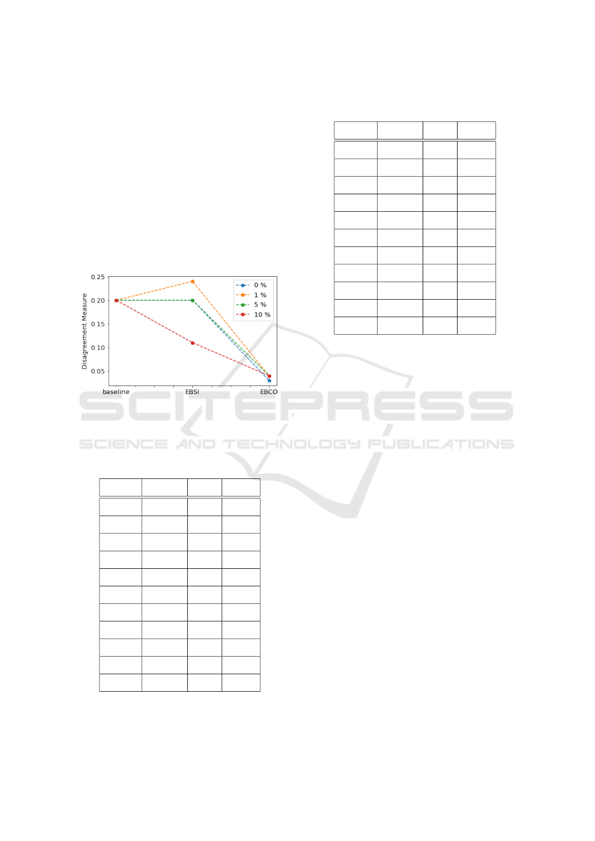
For a deeper analysis, we also studied the evolu-

tion of the disagreement measure proposed by (Shipp

and Kuncheva, 2002). This is the rate of non-common

errors when one model makes the right prediction

and not the other. In other words, it is a measure

ICPRAM 2023 - 12th International Conference on Pattern Recognition Applications and Methods

276

of conﬂict between both models. The results ob-

tained by the model (AU

[ALL]

, T X

[ALL]

), according to

different labeled data rates, are shown in Fig. 4.

First, we can observe that the disagreement measure

for the baseline models is 0.2. In other words, be-

fore co-incrementation, our models satisfy quite well

the independence assumption, necessary condition for

the co-training to work. The ﬁgure also shows that

the EBCO procedure drastically reduced the non-

common error rate converging almost to 0. Thus, co-

incrementation also helped to reduce the common er-

ror rate between models. Consequently, both models

were able to improve their performance and the pro-

cess helped the best model to increase its initial accu-

racy.

Figure 4: Evolution of the non-common error rate through

the different stages of the EBSICO framework, according to

the rate of labeled data.

Table 1: Accuracy measures at different stages of the EB-

SICO framework with 5% of labeled samples - Action

Units.

Model baseline EBSI EBCO

[ALL]

0.946 0.947 0.948

[M]

0.946 0.949 0.953

[W]

0.946 0.939 0.947

[C1]

0.950 0.950 0.962

[C2]

0.931 0.954 0.931

[C3]

0.974 0.974 0.962

[C4]

0.875 0.917 0.958

[C5]

0.950 0.950 0.966

[C6]

0.933 0.933 0.958

[C7]

0.967 0.963 0.949

[C8]

0.911 0.931 0.960

Table 2: Accuracy measures at different stages of the EB-

SICO framework with 5% of labeled samples - Textures.

Model baseline EBSI EBCO

T X

[ALL]

0.811 0.866 0.943

T X

[M]

0.766 0.847 0.939

T X

[W]

0.833 0.894 0.936

T X

[C1]

0.843 0.824 0.931

T X

[C2]

0.713 0.701 0.885

T X

[C3]

0.821 0.833 0.974

T X

[C4]

0.625 0.625 0.958

T X

[C5]

0.891 0.950 0.950

T X

[C6]

0.849 0.840 0.941

T X

[C7]

0.808 0.869 0.944

T X

[C8]

0.752 0.832 0.921

Moreover, our models were overall able to im-

prove their performance on a new distribution of data

by using only a small amount of labeled data. This

is typically a problem of domain adaptation (Csurka,

2017) where distributions of the training and test sets

do not match, as we have here with datasets CFEE

and CK+. In such a conﬁguration the performance at

test time can be signiﬁcantly degraded. However, this

problem is beyond the scope of this paper.

6.6.2 Impact of Personalization

The purpose of this analysis is to evaluate the con-

tribution provided by the personalization solution we

have proposed.

Results showed that AU

[MORPHO]

obtained the

highest accuracy rate compared to AU

[GENDER]

and

[ALL]

(see Table 3). This can be due to the fact that

clustering images according to the morphological cri-

terion allowed subjects with common characteristics

to be optimally isolated into groups. Thus, it allowed

each model to specialize on a group of subjects with

common traits. Indeed, landmark position showed it-

self to be a more robust criterion for data separation

than gender criterion.

On the other hand, comparing AU

[ALL]

with

[GENDER]

and AU

[MORPHO]

, AU

[ALL]

presented the

lowest performance rate, for 5% and 10% of labeled

samples, and the second lowest for 0% and 1%. This

leads to the conclusion that the customization process

increased the robustness of the model.

For further analysis, we also computed the mean

samples numbers per model. AU

[ALL]

contained the

Co-Incrementation: Combining Co-Training and Incremental Learning for Subject-Speciﬁc Facial Expression Recognition

277

largest amount of labeled data since it did not use

data clustering. Considering a label rate of 1%, 5%

and 10%, we computed an average of 4, 22 and 45

labeled samples per chunk for AU

[GENDER]

and an av-

erage of 1, 5 and 11 labeled samples per chunk for

[MORPHO]

(see Table 4). Regardless of the little

amount of labeled data per chunk, AU

[MORPHO]

was

capable of obtaining better performance compared to

[GENDER]

and AU

[ALL]

. As a consequence, we can

deduce that a rationalized clustering strategy provides

robustness during the co-incrementation process, re-

gardless of the number of labeled samples. Therefore,

a rationalized way for the data clustering process is

crucial for models improvements.

The table also shows that thanks to personaliza-

tion, we allow the labelling of fewer images on aver-

age than the generalized AU

[ALL]

model.

Furthermore in Table 1, it was observed that both

AU and T X beneﬁted from co-incrementation. This

conﬁrms our hypothesis that knowledge sharing be-

tween different models leads to improvement of the

prediction rate, regardless of the view and the chosen

clustering criterion.

When several subjects produce the same emotion

differently, as a direct consequence of the identity

bias, this results in a greater intra-class variance. We

observed the evolution of this variance, according to

the separation of the slots according to the personal-

ization criteria that we have presented in the previ-

ous section. The number of slots created depends on

the chosen personalization criteria. In order to make

a fair comparison, we have therefore carried out for

each criterion, except for ALL, a random separation

with the same number of slots. This has been car-

ried out over 100 folds, and the ﬁnal result is the aver-

age of the slot intra-class variances with their standard

deviations. In this way, we distinguish a separation

made on a random criterion from a separation made

on a rational criterion. Moreover, because of the great

number of neutrals, this one was downsampled to 50

to correspond to the distributions of the other labels.

The separation criteria with their associated number

of slots are the following:

Table 3: average accuracy per chunk - EBSICO with Action

Unit view.

% AU

[ALL]

[GENDER]

[MORPHO]

0 0.947 0.946 ± 0.0 0.952 ± 0.013

1 0.948 0.946 ± 0.0 0.952 ± 0.013

5 0.948 0.949 ± 0.003 0.956 ± 0.01

10 0.951 0.954 ± 0.001 0.956 ± 0.01

Table 4: Chunk sizes - EBSICO - Action Unit view.

% |L

ALL

| |L

GENDER

| |L

MORPHO

0 0 0 0

1 9 4 ± 2 1.0 ±1

5 45 22 ± 8 5 ±3

10 90 45±15 11 ± 6

Table 5: Impact of chunking on intra-class variances.

ALL 4.719

RANDOM 2 4.623 ± 0.167

GENDER 2 4.466 ± 0.624

RANDOM 5 4.327 ± 0.353

MORPHO 5 4.211 ± 0.304

RANDOM 8 4.035 ± 0.488

MORPHO 8 3.935 ± 0.483

ALL: 1 slot (whole CK+incr, AUs only),

RANDOM 2: 2 slots, random separation, (average

over 100 folds),

GENDER 2: 2 slots,

RANDOM 5: 5 slots, random separation, (average

over 100 folds),

MORPHO 5: 5 slots,

RANDOM 8: 8 slots, random separation, (average

over 100 folds),

MORPHO 8: 8 slots.

The results are available in the table 5. We can

notice that, the more slots there are, the more the

intra-class variance decreases. In an extreme case

like putting only one subject per slot, the intra-class

variance will tend towards 0. We can thus observe

in the table that the average intra-class variance de-

creases when we constitute more slots with a differ-

ent criterion. These results suggest that as the intra-

class variance decreases, the identity bias is reduced.

Moreover, when comparing the same number of slots,

we observe that the rational separation criterion offers

a slightly lower intra-class variance than the random

criterion. This result conﬁrms, on the one hand, the

quality of these personalization criteria, and on the

other hand, motivates the search for even more reﬁned

rational separation criteria for future experiments.

ICPRAM 2023 - 12th International Conference on Pattern Recognition Applications and Methods

278

Table 6: Comparison of the classical co-training algorithm with our co-incrementation algorithm.

Methods \Metrics acc after L (90) acc after U (811) execution time

classical co-training (0.957,0.888) (0.91, 0.909) 245 min

co-incrementation (0.96,0.897) (0.954, 0.933) 3 min

6.6.3 Comparison of Co-Training and

Co-Incrementation

Finally, we compared our EBSICO algorithm with the

classical co-training algorithm. We used the follow-

ing learning process:

1. training of µ

and µ

respectively on CFEE

[AU]

and CFEE

[T X]

2. the incrementation of the models is done from

CK+

which has been divided to 10% of labels,

so that the numbers are: 90 data for L and 811

data for U, without slots,

3. ﬁrst evaluation of the models after incrementing

on L,

4. then co-train incrementing, with the classical

method (re-training from zero at each iteration)

and our co-incrementing method,

5. second evaluation on CK+

after incrementing on

The accuracies are given in pairs: the ﬁrst one cor-

responds to the AU model, and the second to the T X

model. The conﬁdence threshold has been set at 0.8.

Finally, we compute the total execution time of the se-

quence, in order to compare the classical method and

the incremental method.

The results, comparing the classical co-training

procedure and the one we propose, are presented in

the table 6. We can observe that when a signiﬁcant

number of data in U is present, the classical model

sees its performances decrease drastically, while the

incremental model stagnates, or even improves the µ

model. Finally, the EBSICO procedure that we pro-

pose has a major interest in terms of speed of execu-

tion, nearly 80 times faster in this experiment.

7 CONCLUSION

In this paper, we propose a hybrid method, which

combines two algorithms, namely co-training and in-

cremental learning, allowing two models to collab-

orate and share their knowledge. Compared to the

classical co-training method that performs re-training

from scratch, our approach performs model incremen-

tation continuously on new samples, saving signif-

icant execution time. Another advantage of using

incremental learning over re-training a model from

scratch, in addition to the execution time, is to avoid

”catastrophic forgetting”. NCMFs provide robust re-

sistance to models trained several steps earlier.

Second, in this paper we provide an in-depth anal-

ysis of model personalization for emotion recogni-

tion. Models taking into account morphological fea-

tures have shown better performance versus cluster-

ing by gender. Indeed, a rationalized technique for

feature clustering is crucial for co-training model per-

formance.

Finally, our third contribution concerns the ﬁeld

of semi-supervised learning, more speciﬁcally, on the

ability of models to increase their performance with

only 5% of labeled samples, as demonstrated in our

experiments. Our experiments have been conducted

with small datasets, but we could imagine in fu-

ture research work using this technique with larger

databases.

REFERENCES

Baltru

saitis, T., Robinson, P., and Morency, L.-P. (2016).

Openface: an open source facial behavior analysis

toolkit. In 2016 IEEE Winter Conference on Applica-

tions of Computer Vision (WACV), pages 1–10. IEEE.

Blum, A. and Mitchell, T. (1998). Combining labeled and

unlabeled data with co-training. In Proceedings of the

eleventh annual conference on Computational learn-

ing theory, pages 92–100.

Breiman, L. (2001). Random Forests. Machine Learning,

45(1):5–32.

Chu, W.-S., De la Torre, F., and Cohn, J. F. (2013). Se-

lective transfer machine for personalized facial action

unit detection. In Proceedings of the IEEE Conference

on Computer Vision and Pattern Recognition, pages

3515–3522.

Cohen, I., Sebe, N., Cozman, F. G., and Huang, T. S. (2003).

Semi-supervised learning for facial expression recog-

nition. In Proceedings of the 5th ACM SIGMM in-

ternational workshop on Multimedia information re-

trieval, pages 17–22.

Csurka, G. (2017). Domain adaptation for visual appli-

cations: A comprehensive survey. arXiv preprint

arXiv:1702.05374.

Denil, M., Matheson, D., and Freitas, N. (2013). Con-

sistency of online random forests. In International

conference on machine learning, page 1256–1264.

PMLR.

Co-Incrementation: Combining Co-Training and Incremental Learning for Subject-Speciﬁc Facial Expression Recognition

279

Du, S., Tao, Y., and Martinez, A. M. (2014). Compound

facial expressions of emotion. Proceedings of the Na-

tional Academy of Sciences, 111(15):E1454–E1462.

Ekman, R. (1997). What the face reveals: Basic and applied

studies of spontaneous expression using the Facial Ac-

tion Coding System (FACS). Oxford University Press,

USA.

Gonzalez, J. and Prevost, L. (2021). Personalizing emo-

tion recognition using incremental random forests. In

2021 29th European Signal Processing Conference

(EUSIPCO), pages 781–785. IEEE.

Hastie, T., Tibshirani, R., and Friedman, J. (2009). The el-

ements of statistical learning: data mining, inference,

and prediction. Springer Science & Business Media.

Hu, C., Chen, Y., Hu, L., and Peng, X. (2018). A

novel random forests based class incremental learning

method for activity recognition. Pattern Recognition,

78:277–290.

Kollia, V. (2016). Personalization effect on emotion recog-

nition from physiological data: An investigation of

performance on different setups and classiﬁers. arXiv

preprint arXiv:1607.05832.

Lakshminarayanan, B., Roy, D. M., and Teh, Y. W. (2014).

Mondrian forests: Efﬁcient online random forests.

Advances in neural information processing systems,

27:3140–3148.

Lucey, P., Cohn, J. F., Kanade, T., Saragih, J., Ambadar,

Z., and Matthews, I. (2010). The extended cohn-

kanade dataset (ck+): A complete dataset for action

unit and emotion-speciﬁed expression. In 2010 ieee

computer society conference on computer vision and

pattern recognition-workshops, pages 94–101. IEEE.

Meng, Z., Gaur, Y., Li, J., and Gong, Y. (2019).

Speaker adaptation for attention-based end-to-end

speech recognition. arXiv preprint arXiv:1911.03762.

Oudot, L., Prevost, L., Moises, A., and Milgram, M.

(2004). Self-supervised writer adaptation using per-

ceptive concepts: Application to on-line text recogni-

tion. In Proceedings of the 17th International Confer-

ence on Pattern Recognition, 2004. ICPR 2004., vol-

ume 3, pages 598–601. IEEE.

Provost, F. and Domingos, P. (2003). Tree induction

for probability-based ranking. Machine learning,

52(3):199–215.

Quinlan, J. R. (1986). Induction of decision trees. Machine

learning, 1(1):81–106.

Ristin, M., Guillaumin, M., Gall, J., and Van Gool, L.

(2014). Incremental learning of ncm forests for large-

scale image classiﬁcation. In Proceedings of the IEEE

conference on computer vision and pattern recogni-

tion, page 3654–3661.

Sariyanidi, E., Gunes, H., and Cavallaro, A. (2014). Au-

tomatic analysis of facial affect: A survey of regis-

tration, representation, and recognition. IEEE trans-

actions on pattern analysis and machine intelligence,

37(6):1113–1133.

Senechal, T., Bailly, K., and Prevost, L. (2010). Auto-

matic facial action detection using histogram varia-

tion between emotional states. In 2010 20th Inter-

national Conference on Pattern Recognition, pages

3752–3755. IEEE.

Settles, B. (2009). Active learning literature survey.

Shipp, C. A. and Kuncheva, L. I. (2002). Relationships

between combination methods and measures of di-

versity in combining classiﬁers. Information fusion,

3(2):135–148.

Tanha, J., van Someren, M., and Afsarmanesh, H. (2017).

Semi-supervised self-training for decision tree classi-

ﬁers. International Journal of Machine Learning and

Cybernetics, 8(1):355–370.

Wang, W. and Zhou, Z.-H. (2010). A new analysis of co-

training. In ICML.

Yang, S. and Bhanu, B. (2011). Facial expression recog-

nition using emotion avatar image. In 2011 IEEE In-

ternational Conference on Automatic Face & Gesture

Recognition (FG), pages 866–871. IEEE.

Zhang, Z., Ringeval, F., Dong, B., Coutinho, E., Marchi, E.,

and Sch

uller, B. (2016). Enhanced semi-supervised

learning for multimodal emotion recognition. In 2016

IEEE International Conference on Acoustics, Speech

and Signal Processing (ICASSP), pages 5185–5189.

IEEE.

Zhou, Z.-H. (2018). A brief introduction to weakly super-

vised learning. National science review, 5(1):44–53.

Zhou, Z.-H. and Li, M. (2010). Semi-supervised learning by

disagreement. Knowledge and Information Systems,

24(3):415–439.

ICPRAM 2023 - 12th International Conference on Pattern Recognition Applications and Methods

280