DeNos22: A Pipeline to Learn Object Tracking Using Simulated Depth

Dominik Penk

, Maik Horn

, Christoph Strohmeyer

, Frank Bauer

and Marc Stamminger

Chair of Visual Computing, Friedrich-Alexander-Universit

at Erlangen-N

urnberg, Cauerstraße 11, Erlangen, Germany

Schaefﬂer Technologies AG & Co. KG, Industriestraße 1-3, Herzogenaurach, Germany

ﬂ

Keywords:

6D Pose Estimation, Object Tracking, Depth Simulation, Machine Learning, Robust Estimators.

Abstract:

We propose a novel pipeline to construct a learning based 6D object pose tracker, which is solely trained on

synthetic depth images. The only required input is a (geometric) CAD model of the target object. Training data

is synthesized by rendering stereo images of the CAD model, in front of a large variety of backgrounds gen-

erated by point-based re-renderings of prerecorded background scenes. Finally, depth from stereo is applied

in order to mimic the behavior of depth sensors. The synthesized training input generalizes well to real-world

scenes, but we further show how to improve real-world inference using robust estimators to counteract the

errors introduced by the sim-to-real transfer. As a result, we show that our 6D pose trackers achieve state-of-

the-art results without any annotated real-world data, solely based on a CAD-model of the target object.

1 INTRODUCTION

Object pose estimation for known objects is an inte-

gral part of many tasks, ranging from visual inspec-

tion to augmented reality applications. Despite its

importance, robust and global solutions to this prob-

lem were not available until the emergence of learn-

ing based pose estimation approaches in recent years.

These methods require a large amount of training

data, RGB(-D) images with associated object poses,

to be properly trained. The labeling process is partic-

ularly tedious and time-consuming since navigating a

3D environment and manually ﬁtting an object pose

is unintuitive for most users.

In this paper, we present a pipeline to bootstrap a

depth-based object pose tracker, which does not need

any manually labeled data. The bootstrapping only

requires the geometric CAD data of the object. We do

neither require nor use any kind of real-world train-

ing data or manually crafted labels. Training relies

purely on synthetic depth images, which ensures that

we can produce an exhaustive amount of training data

without any user interaction.

We prefer depth images over RGB images as in-

put for pose estimation for a simple reason: Synthe-

sizing RGB images as training data is a highly desir-

able goal, but also particularly difﬁcult. Many effects,

like environmental illumination, specular highlights,

or object albedo, have a strong impact on the ﬁnal re-

sult. Thus, these effects need to be modeled, which

makes it necessary to have material properties and

textures of the target object. This kind of data is not

available in most industrial applications. Depth im-

ages on the other hand exclusively contain geometric

information, which can be synthesized using a CAD

model only. They are also less inﬂuenced by envi-

ronmental and object speciﬁc attributes. We present a

pipeline for the generation of training data for depth-

based pose estimation in Section 3. Pose estimation

trained on our synthesized depth images generalizes

relatively well to real-world data, nevertheless a sim-

to-real domain gap remains. We address this in Sec-

tion 4 by postprocessing and ﬁltering the network pre-

dictions to improve performance. We evaluate this ap-

proach in Section 5 and show that we perform on par

with prior work.

While we present an object tracking network, a

major aspect of our contribution is the proposed syn-

thesis of training data. That data can be employed to

train a variety of other object-related tasks. This ex-

tends the utility of our training approach to various

other applications.

2 RELATED WORK

The ﬁeld of 6D pose estimation contains a large body

of work. Here, we will give a short overview of some

subﬁelds that are closely related to this work.

Penk, D., Horn, M., Strohmeyer, C., Bauer, F. and Stamminger, M.

DeNos22: A Pipeline to Learn Object Tracking Using Simulated Depth.

DOI: 10.5220/0011635100003417

In Proceedings of the 18th International Joint Conference on Computer Vision, Imaging and Computer Graphics Theory and Applications (VISIGRAPP 2023) - Volume 5: VISAPP, pages

953-962

ISBN: 978-989-758-634-7; ISSN: 2184-4321

 2023 by SCITEPRESS – Science and Technology Publications, Lda. Under CC license (CC BY-NC-ND 4.0)

953

DeNos22

Training Pose Estimation

Final Pose

ICP

Tracking

Pose

Filter

RANSAC

Pose Fitting

NOS Map

DeNos22

CAD Model

Depth Image

Reference Output

Input Data

randomized

Data Synthesis

NOS Map

Pixel Mask

Depth Image

Synthesized Data

randomized

Postprocessing

Virtual

Depth

Camera

randomized

IR Projection

randomized

Env. Lighting

3D World

Background

CAD Model

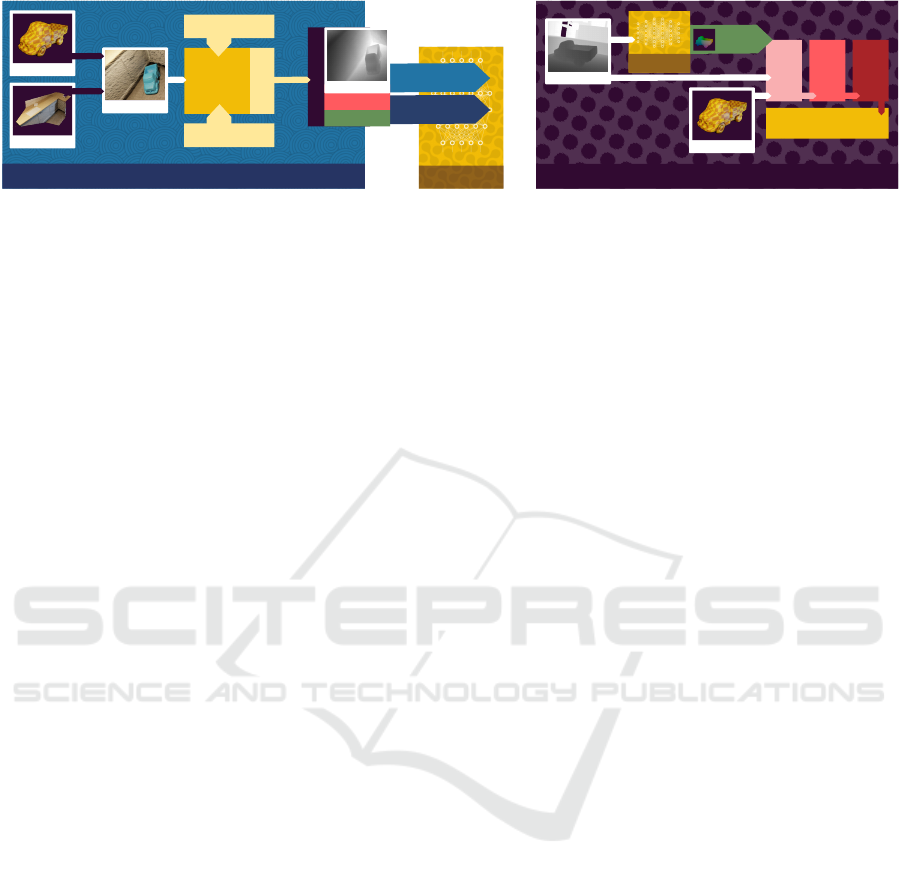
Figure 1: Our proposed pipeline spans the tracker bootstrapping phase and productive use. During setup, we automatically

generate training data for the learning based pose estimate. In production, we deal yield high quality ﬁnal poses, by using

robust estimators and model-based ﬁltering, despite the sim-to-real gap.

2.1 Local Approaches

Methods in this category expect a CAD model of

the tracked object, an initial rough pose estimation

plus some observation. Probably the most widely

used representative is the iterative closest point (short

ICP) method introduced by (Chen and Medioni,

1992; Besl and McKay, 1992) and its many variants

(Rusinkiewicz and Levoy, 2001). We want to speciﬁ-

cally mention the projective ICP variant introduced by

(Newcombe et al., 2011) which drastically simpliﬁes

the point matching process and is used in this work.

Besides depth or point-cloud observations there are

also methods relying on color images only e.g. (Col-

let et al., 2011).

In general, these methods generate high quality

poses. Unfortunately, the initial pose estimation is a

hard limitation for their practical use, which implies

that these method are often used as a post-processing

step.

2.2 Global Approaches

Methods in this category try to provide a 6D pose

without any prior initialization, which is a much

harder problem compared to the local approach. Clas-

sic approaches commonly rely on handcrafted feature

matches (Birdal and Ilic, 2015; Drost et al., 2010)

between CAD model and an observed point cloud.

Closer related to this work are a large amount of data

driven methods introduced in the last couple of years

that aim to solve 6D pose estimation using neural net-

works. One interesting observation is that a large

portion of these methods try to directly regress the

6D pose on RGB images. One of the ﬁrst success-

ful approaches in this direction is PoseCNN (Xiang

et al., 2017) which inspired a multitude of similar ap-

proaches (Do et al., 2018; Liu et al., 2019; Liu and

He, 2019).

One major hurdle for any direct regression method

is the representation of rotation, which greatly im-

pacts training speed and the ﬁnal pose quality. (Kehl

et al., 2017) and (Sundermeyer et al., 2018) propose

to convert direct regression in SO(3) into a classi-

ﬁcation problem. However, a simple discretization

into 5° bins yield upwards of 50.000 classes (Sunder-

meyer et al., 2018). As an alternative, some authors

propose complex class generation based on auto en-

coders (Sundermeyer et al., 2020; Sundermeyer et al.,

2018) or viewport proposals (Kehl et al., 2017). On

the other hand, (Zhou et al., 2019) proposes that all

common rotation representations, such as Euler an-

gles or quaternions, are discontinuous in euclidean

space. This inhibits training of neural networks and

they therefore introduce 5D and 6D rotation represen-

tations that are better suited for learning.

Another line of work circumvents these difﬁcul-

ties using a multi stage approach, where per pixel

object space coordinates are found, which are then

used to infer object pose information. Applications of

these method range from body pose estimation (G

uler

et al., 2018) to camera localization (Shotton et al.,

2013). Our method is based on these approaches

which were already applied for instance pose estima-

tion by (Brachmann et al., 2014) and extended to ob-

ject class level pose estimation (Wang et al., 2019).

2.3 Depth Synthesis

Generating high quality synthetic training data is an

active research topic. The task is especially difﬁ-

cult for RGB data since many real world occurrences,

like lighting or surface properties, must be incorpo-

rated. In this work we try to forgo some of these dif-

ﬁculties by using depth maps instead. Both (Landau

et al., 2015) and (Planche et al., 2017) propose ex-

tensive frameworks to simulate a speciﬁc multi-view

stereo depth sensor as realistically as possible. Simi-

lar works are also available for time of ﬂight sensors

(Keller and Kolb, 2009; Peters and Loffeld, 2008).

Our depth simulation is also tailored to multi-view

stereo sensors and primarily inspired by (Planche

et al., 2017). In order to create an easy to use and

adaptable pipeline we choose to produce semi realis-

VISAPP 2023 - 18th International Conference on Computer Vision Theory and Applications

954

(a) (b)

Figure 2: Depth simulation parameters effect the resulting

depth in different ways. (a) compares the results of block

matching (top) to semi global matching (bottom). Render

settings often lead to less obvious changes in the result-

ing depth. (b) visualizes the resulting depth under changing

lighting projector patterns.

tic depth images. With automated domain randomiza-

tion the trained network nevertheless generalizes well

to different sensors.

A research ﬁeld closely related to depth simula-

tion is the generation of realistic RGB(-D) images.

Some works use these images to train pose detec-

tion networks, e.g. BlenderProc by (Denninger et al.,

2020) or (Hinterstoisser et al., 2019). In contrast to

our method, these rely on textured meshes and ap-

proximated material properties, which may compli-

cate practical usage.

3 TRAINING DATA SYNTHESIS

At ﬁrst, our pipeline generates synthetic data to train

a pose estimation network. We aim to create a dataset

containing realistic depth images of the target ob-

ject under varying pose in different environments, to-

gether with all required labels.

Similar to (Planche et al., 2017), we simulate the

depth acquisition process of a stereo camera. This en-

sures that common artifacts of consumer grade RGB-

D cameras such as occlusions and noise are present

in the simulated data. The simulation process is vi-

sualised in the left box of Fig. 1 and consists of two

steps: The scene assembly creates a randomized vir-

tual scene showing the target object in random pose

in front of a plausible, but randomized background.

A virtual stereo camera then captures the scene and

produces the ﬁnal depth image together with other re-

quired ground truth data. Both steps are detailed in

this section.

Figure 3: Results of our simulation pipeline. From left to

right: The intermediate, rendered left stereo image, the nos

framebuffer and ﬁnally the computed depth.

3.1 Scene Assembly

The task of the scene assembly stage is to construct

a set of virtual scenes that sample the real world ade-

quately. This includes, most importantly, varying ob-

ject poses, but also backgrounds and secondary ef-

fects like partial occlusion. To obtain realistic vir-

tual backgrounds, we use a set of RGB-D images of

real world scenes. This is preferred over virtually

created environments, since creating realistic back-

grounds using purely virtual assets is time consum-

ing. Instead, we can easily capture multiple different

views of representative environments using an RGB-

D camera, and increase variation by rendering these

RGB-D images from different perspectives (see next

section). For our examples we use a publicly available

dataset of tables (Wang et al., 2019).

We start the scene assembly with a randomly se-

lected background and place some instances of the

target object into it. In our use cases the tracked ob-

jects are commonly placed on table surfaces, which

we integrated into our assembly process: We extract

large planar regions in the depth map and ensure that

objects always spawn in these regions. To further

increase pose variety we have to rotate the objects

randomly, however, most rotations are not physically

plausible. Instead we compute the convex hull and ro-

tate the object such that a random hull triangle aligns

with the table surface.

Since the background scenes are quite clean we

randomly select additional distractor objects from the

ShapeNet (Chang et al., 2015) dataset and also place

them into the scene.

Finally we place the virtual (stereo) camera to cap-

ture the assembled environment. We also make sure

that the relative position of the camera and the tar-

get objects are similar plausible. This mostly comes

down to a reasonable camera-object distance and

viewing angle (e.g. mostly overhead shots or surface

aligned camera poses).

3.2 Virtual Stereo Rendering

To generate a realistic depth image of our assembled

scene, we closely resemble the computation pipeline

DeNos22: A Pipeline to Learn Object Tracking Using Simulated Depth

955

Central

Differences

Instance Mask

NOS Map

Region Proposal Detection Heads

Depth

ROI Align

conv

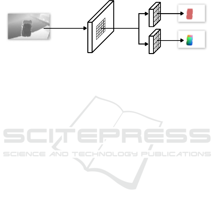
Figure 4: The DeNos22 architecture computes the ﬁrst order derivative of the input depth using central differences and passes

it to the region proposal network. This network generates regions of interest which are processed by two detection heads to

generate nos maps and per pixel instance masks.

as it is used in similar form in RGB-D cameras: ﬁrst,

two cameras capture an image pair which is, second,

rectiﬁed for further processing. Third, corresponding

pixels are matched to compute a disparity map. Fi-

nally, postprocessing ﬁlters are applied, e.g. for hole

ﬁlling. To improve the ﬁnding of correspondences,

most modern RGB-D cameras add high contrast pat-

terns into the scene using a built-in infrared projec-

tor. Some systems use one camera only, and include

knowledge about the projected pattern. We ignore this

case, since the resulting artifacts are similar to a stereo

camera.

The Virtual Stereo Camera block in Fig. 1 resem-

bles this process virtually. We combine image acqui-

sition and rectiﬁcation by directly rendering perfectly

aligned images and apply correspondence ﬁnding and

postprocessing as in real-world depth estimation.

To synthesize the two views, we ﬁrst render the

chosen captured background scene with point based

rendering (Botsch and Kobbelt, 2003), which allows

us to change perspective for stereo rendering, as well

as to randomize backgrounds. Subsequently, we ras-

terize the placed objects—both target and distractor—

using OpenGL. We use simple Phong shading based

rendering and forego more realistic shading methods

that could imitate secondary effects like reﬂections.

Similar to (Planche et al., 2017), we simulate the IR

projectors with a textured spotlight. To achieve realis-

tic lighting gradients on the CAD model we use spher-

ical harmonics as environmental illumination. Since

the point clouds are captured from real data, they are

already illuminated, and we only add lighting from

the virtual IR projector.

For each image pair we randomize as many render

settings as possible to capture a wide variety of possi-

ble scenarios. This includes drawing random illumi-

nation coefﬁcients from the Basel illumination prior

(Egger et al., 2018), varying albedo colors and specu-

lar expontents. The exact IR patterns are proprietary,

but are in general semi-random dot patterns or white

noise textures. We therefore generate different dot

patterns using Halton Sequences with random basis.

Note that the goal is not to generate photo-

realistic images—instead the renderings are immedi-

ately passed to a stereo reconstruction pipeline im-

plemented using OpenCV to obtain a realistic depth

map with typical artifacts. In this ﬁnal step we ap-

ply algorithmic randomization by picking different

stereo matching methods and postprocessing parame-

ters. Figure 2 shows how the rendering and algorith-

mic randomizations impact the ﬁnal depth map for the

same virtual scene. In general, algorithmic settings

inﬂuence the ﬁnal result the most. Render settings,

on the other hand, have a more subtle inﬂuence on the

synthesized depth maps.

With the proposed method we generate ground

truth data including per-pixel labels. The depth im-

ages from the stereo pipeline are perfectly aligned

with the left camera image by construction. There-

fore, any data we output to an additional framebuffer,

while rendering the left camera image, will also be

pixel perfect.

Of particular interest for this paper are per-pixel

correspondences between real world depth and posi-

tion on the CAD surface in object space coordinates

. We normalize these by the axis aligned bounding

box of the target object to produce normalized object

space coordinates ˜p

(short nos coordinates). This en-

sures a value range that is independent of the object

size and is also easy to convert to an RGB image. Re-

construction of the original coordinates is achieved by

VISAPP 2023 - 18th International Conference on Computer Vision Theory and Applications

956

inverting the normalization:

= p

min

+ ˜p

⊙ (p

max

− p

min

) (1)

Here p

min

and p

max

are the extrema of the CAD

model’s bounding box and ⊙ symbolises the element-

wise product.

In Fig. 3 we depict for an example scene the inter-

mediate rendered color, the corresponding nos coor-

dinate and simulated depth map.

4 DeNos22

We adopt a two stage approach for initial pose esti-

mation. A neural network, which we call DeNos22,

receives depth frames and estimates per pixel instance

mask and nos values, which we regress to the initial

pose estimate.

By construction, we know that the predicted nos

coordinate at pixel (u, v) corresponds to the depth

value at the same image location. From these corre-

spondences we can recover the object rotation R and

translation t by minimizing

argmin

R,t

∑

(u,v)∈M

(u, v) − Rp

(u, v) −t)

(2)

with the orthogonal Procrustes method. Here, (u,v) ∈

M refers to all pixels with valid depth values covered

by the object and p

is the network prediction denor-

malized using Eq. (1). p

is the world space position

we receive by unprojecting the depth at pixel (u, v)

using the depth cameras intrinsic parameters.

4.1 Architecture

The DeNos22 architecture is depicted in Fig. 4 and

originates from the one proposed by (Wang et al.,

2019).

Instead of color images we use the ﬁrst order

derivative of the depth, computed using central differ-

ences, as input. Using the derivative prevents the net-

work from identifying objects purely based on the dis-

tance to the camera. Our model is based on the pop-

ular Mask R-CNN framework (Doll

ar and Girshick,

2017) which has two main stages. First, a region pro-

posal network predicts bounding boxes of foreground

objects and produced feature maps from the input im-

age. In the second stage, the regions of interest are

extracted from the feature maps, reshaped to a com-

mon size and passed to multiple detection heads for

further processing. We use the instance mask and

nos prediction but drop the classiﬁcation head and as-

sume all foreground objects produced by the region

proposal are valid. The reduced network size did not

Figure 5: RANSAC (center) and least square pose (right)

extracted from a wrongly labeled network prediction. The

RANSAC approach still yields a pose that ﬁts the observed

depth.

lead to a decrease in classiﬁcation accuracy in our ex-

periments, but reduces training time and increases in-

ference speed.

We train the DeNos22 network with the synthetic

data produced in Section 3 in a supervised fashion.

Similar to (Wang et al., 2019) we do not directly

regress the nos coordinates. Instead, we subdivide

each axis of the unit cube into 32 bins and task the

network to classify to which one a given image pixel

belongs. With this formulation the DeNos22 essen-

tially estimates a three dimensional voxel index with

independent classiﬁcation tasks. During inference we

use the center of the estimated voxel as an approxi-

mation of the continuous nos coordinate.

4.2 Robust Estimators

In productive use, noisy depth maps and erroneous

nos predictions—which partially originate from the

domain caused by virtual training—decrease the ac-

curacy of the estimated pose. We also observed that

the region proposal stage sometimes outputs false

foreground predictions.

Our network yields many, semi independent, pre-

dictions per observed instance I. Therefore, we can

employ a RANSAC-style method to improve the pose

estimates. For each instance we randomly sample

multiple small subsets M

from the set of all pre-

dicted nos coordinates M

. From those, we predict

rotations R

and translations t

according to Eq. (2).

We rate each pose by computing the number of inlier

pixels based on the virtual compared to the observed

depth (

and d):



(u, v) − d(u, v)



< δ (3)

where δ is a small threshold (e.g. 1cm). We obtain

from the depth buffer after rendering the CAD model

using the pose (R

As depicted in Fig. 5 the proposed method often

yields plausible results, even for wrongly classiﬁed

DeNos22: A Pipeline to Learn Object Tracking Using Simulated Depth

957

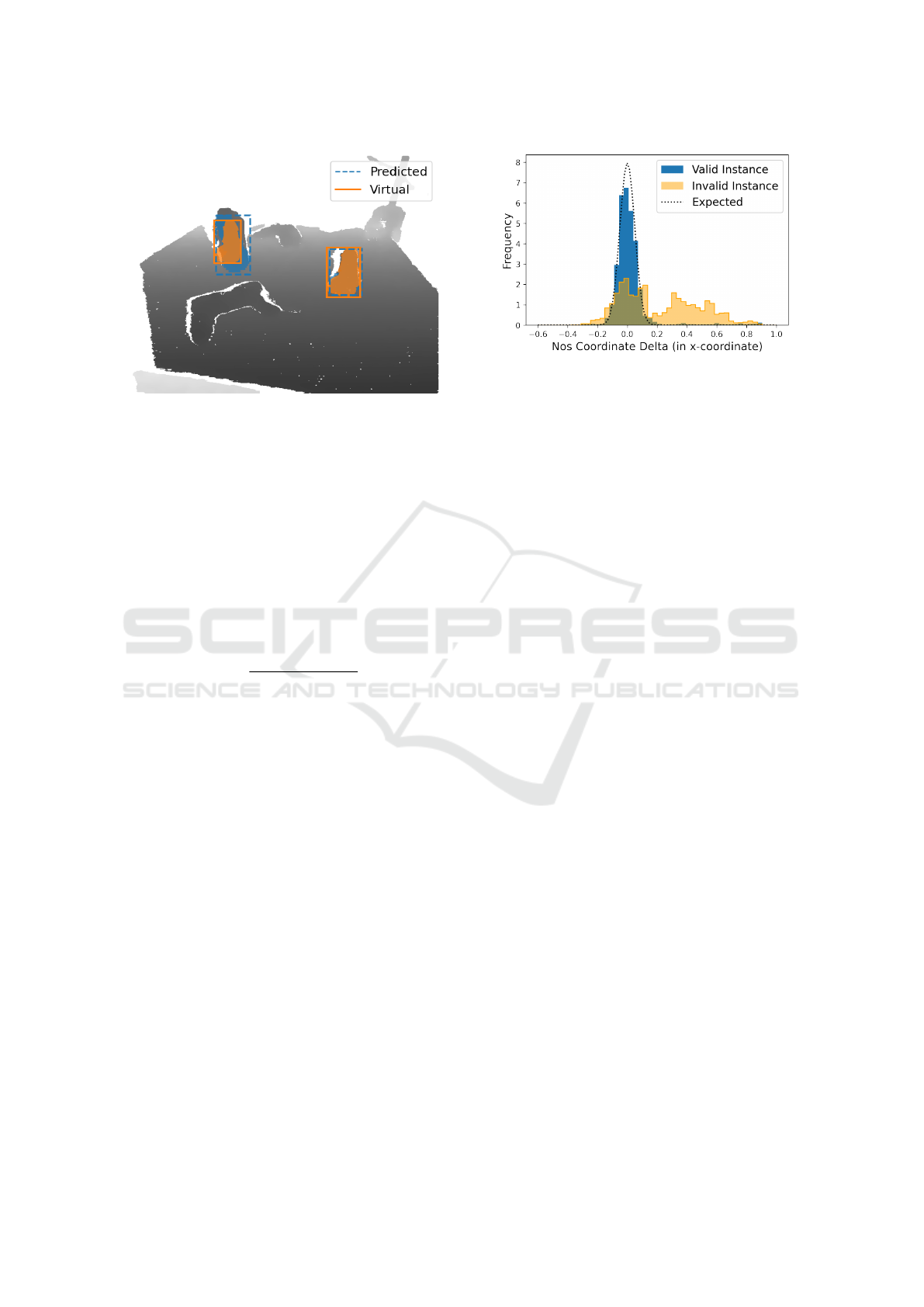
Figure 6: The bounding box of the rendered object and the

one predicted by DeNos22 match for valid instances (right)

and are often vastly different for invalid ones (left).

foreground regions. This implies the inlier count can-

not be used to identify invalid network predictions. In

a second step, we therefore ﬁlter out invalid instances

using two quality metrics, For the ﬁrst, we compute

the image space bounding box bb

of the object given

the estimated pose. This bounding box should match

the one predicted by the network bb

net

, but we ob-

served that this is often not the case for invalid in-

stances, see Fig. 6. This can be described by the in-

tersection over union:

IoU

area(bb

∩ bb

net

)

area(bb

∪ bb

net

)

(4)

Since DeNos22 only produces a bounding box around

the object’s visual parts, we must ensure that the pro-

jected bounding box takes occlusion into account.

This is done by rendering the object and comparing

the depth buffer against the observed depth. In fact,

the required data was already produced to count the

inliers in Eq. (3), so we can reuse it to increase per-

formance.

The second metric is a purely model-based mea-

sure. We assume that the difference between the

network-predicted and simulated nos coordinates

net

and q

) is normal-distributed with a zero mean.

In Fig. 7 we show two exemplary distributions (along

a singular dimension). Since the network calculates

the nos coordinate axes independently, we also as-

sume that modalities of the distributions are indepen-

dent. Under these assumptions, we use the Frobenius

norm of the variance to qualify the nos coordinates of

an instance by

nos

= 1.0 −

Var(q

net

− q

)

(5)

The ﬁnal instance score combines both metrics

= Q

nos

IoU

(6)

Figure 7: The graphs show the difference of rendered and

estimated nos coordinates for two predictions. For a correct

instance (right) these closely follow a normal distribution

centered at 0.

covers the range [−∞, 1]. In most of our tests we

dropped instances with a quality below 0.45.

4.3 Pose Reﬁnement

Up to this point, we have shown how to use the

DeNos22 network to obtain a rough estimate for the

pose. (Wang et al., 2019) demonstrated that a ﬁnal

reﬁnement step can be used to further improve accu-

racy.

Since we have a CAD model of the object, we im-

prove the estimation of the network using the ICP

method. We use projective correspondences intro-

duced by (Newcombe et al., 2011) which where used

to align two depth maps. To use the framework, we

render the virtual depth with an estimated pose as well

as the real depth map. At its core, the method reduces

the point to plane error given a transformation (R,t):

argmin

R,t

∑

i∈M





+t − p





(7)

Here, p

and p

are two world points from the unpro-

jected depth maps and M is a set of pixels, where both

maps contain valid depth data. Similar to Eq. (4) we

have to ensure that M does not include occluded parts

of the CAD model. We do so by dropping matches

where depth values differ too much. This threshold

is crucial for good convergence and high quality ﬁnal

poses—low values leads to fewer matches and higher

values fail to remove invalid matches. Since the initial

pose is already close, we skew towards a low thresh-

old in our experiments. A value between 5mm and

2cm yielded good results.

Intuitively, we would use the virtual depth to com-

pute p

, however this requires to estimate the normals

of the real depth map. These are noisy and we in-

stead compute the inverse transformation—aligning

the depth to the CAD model. With this formulation,

VISAPP 2023 - 18th International Conference on Computer Vision Theory and Applications

958

we use the high quality CAD model normals and do

not introduce additional errors into the optimization.

Many applications track an object through an en-

tire sequence of depth maps. In this case, initial

pose estimation using DeNos22 may be too slow. We

recommend to run the complete pipeline, including

pose reﬁnement at the beginning. For all subsequent

frames, the previous pose can be used to initialize the

ICP algorithm.

5 POSE ESTIMATION QUALITY

In this section we evaluate our 6D pose estimator

trained purely on synthetic data. We evaluate both

on the publicly available LM dataset introduced by

(Hinterstoisser et al., 2012), as well as our own data.

For evaluation we trained the network on datasets

containing 8000 images with 1 to 10 instances of the

target object. While the LM dataset includes albedo

textures, we generated our synthetic data using exclu-

sively the geometry data and a public dataset of RGB-

D backgrounds to imitate a usecase with little real

world data. For training, we use SGD with a learning

rate of 0.001 and two images per batch and terminate

optimization after 100 epochs.

In Table 2 we list the average recall values for

pose-error-functions presented in the BOP 6D pose

detection challenge (Hoda

n et al., 2020) for a subset

of all available classes. We used our pipeline to train

a separate DeNos22 per class and the ﬁnal row of the

table displays the average value over all classes. Our

pipeline performs best in terms of the visible surface

discrepancy AR

V SD

. It measures the per-pixel differ-

ence of rendered depth maps using ground truth and

estimated pose. Note that the local projective ICP

uses a similar optimization criterion. This implies that

a different local pose estimator—tailored to a differ-

ent metric—can be used depending on the use case.

Table 1 shows that our method performs on par

with other state-of-the-art methods, even ones which

use additional input information in form of RGB-D

images. For evaluation we apply pose ﬁltering under

the assumption that an image contains a maximum of

one object instance per class.

We also conduct a small ablation study to investi-

gate the importance of the steps in our pipeline. The

results are compiled in Table 3. We conclude that the

robust pose estimation has a major impact on the ﬁnal

pose quality. This supports our choice to estimate an

intermediate rotation representation which we regress

manually over a network that directly estimates the

object pose.

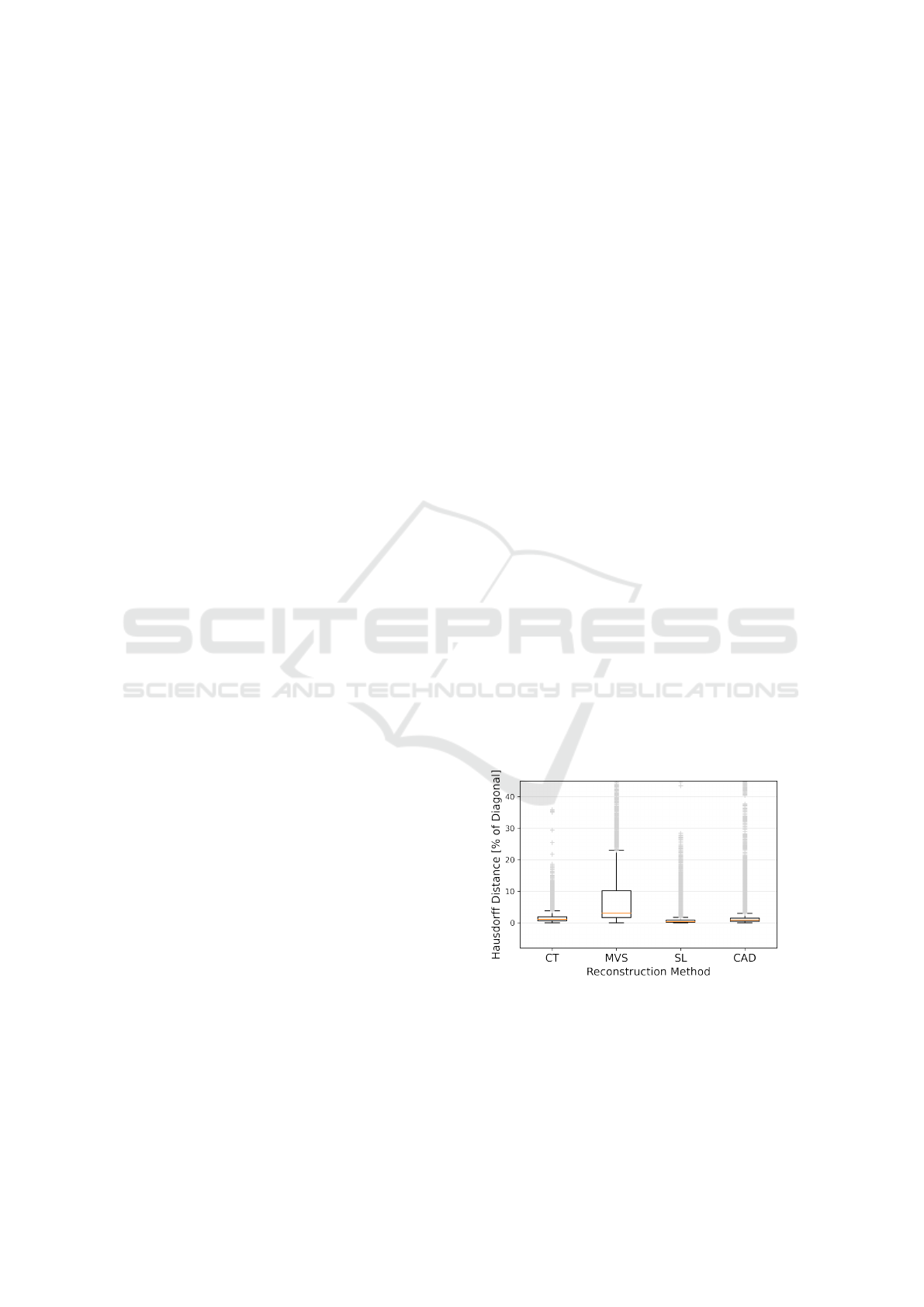
Finally, we evaluate the impact of virtual model

acquisition modality on our pipeline. We gathered 9

different objects and produced virtual representations

of them. The CAD models where reconstructed by a

method yielding the best results, including computer

tomography (CT), multi-view-stereo (MVS) or struc-

tured light (SL) reconstruction. We also include two

objects of which we found public, hand crafted, CAD

models. For this evaluation the ground truth pose is

unknown, we therefore rely on an image space metric

inspired by AR

V SD

: We render the CAD model using

the estimated pose and compute the symmetric Haus-

dorff distance between the real and estimated depth

images inside a manually painted visibility mask. In

Fig. 8 we show these per pixel distances in relation

to the object bounding boxes grouped by the differ-

ent acquisition methods. From the plot we can see

that the poses for structure SL reconstructed objects

are highly accurate, whereas MVS-based objects pre-

formed worse. In Fig. 9 we can see two reconstruc-

tions with these methods. The matchbox car was re-

constructed using MVS and is partially noisy, espe-

cially in the highly specular window regions and the

bottom. In contrast, the head ﬁgure produced by an

SL scanner shows next to no surface inaccuracies.

We conclude that mesh quality is the main reason for

the difference in pose accuracy. The relation between

pose and mesh quality is plausible, as the CAD model

is integral to all steps of our pipeline. With more

accurate models, we naturally generate more plausi-

ble depth maps for training. We also induce smaller,

model-based errors during pose estimation. This ap-

plies to both, the RANSAC rating and the optimiza-

tion target for the projective ICP.

Figure 8: Hausdorff distance between observed and esti-

mated depth maps for a variety of objects.

6 CONCLUSION

We presented a pipeline to construct a learning based

object tracker from just a CAD model. Our pipeline,

DeNos22: A Pipeline to Learn Object Tracking Using Simulated Depth

959

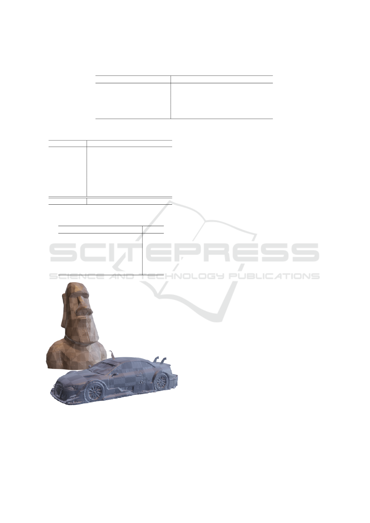
Table 1: Comparison between our pipeline and state of the art methods on the LM-dataset. The cursive written methods

expect RGB-D input, the others expect just depth.

Method AR

V SD

MSSD

MSPD

Ours 0.875 0.814 0.648 0.779

PPF (Deng, 2022) 0.719 0.856 0.866 0.814

RCVPose (Wu et al., 2021) 0.740 0.826 0.832 0.799

FFB6D (He et al., 2021) 0.673 0.810 0.835 0.773

MGML (Drost et al., 2010) 0.678 0.786 0.789 0.751

Table 2: Average recalls w.r.t. the error metrics deﬁned by

the BOP challenge.

Object A

V SD

MSSD

MSPD

Statue 0.968 0.912 0.793 0.891

Watering Can 0.652 0.620 0.498 0.590

Kitten 0.949 0.939 0.834 0.908

Screwdriver 0.862 0.837 0.691 0.797

Duck 0.962 0.886 0.717 0.855

Egg Carton 0.947 0.929 0.794 0.890

Glue Bottle 0.765 0.701 0.412 0.626

Puncher 0.892 0.689 0.443 0.675

Average 0.875 0.814 0.648 0.779

Table 3: Average recalls on the LM-dataset for our pipeline

with different parts of the pipeline disabled.

Distractors RANSAC ICP AR

% ✓ ✓ 0.714

✓ % % 0.608

✓ % ✓ 0.666

✓ ✓ % 0.740

✓ ✓ ✓ 0.779

Figure 9: Two samples from of our reconstructed objects.

The matchbox car model was created using multi view

stereo which yields noisy surfaces, e.g. the windows. In

contrast the head statue shows very little noise and was ac-

quired with a structured light scan.

generates a large amount of training data by rendering

stereo images of the object and reconstructing depth

images from these, which results in typical depth

camera artifacts. The large variation in our synthet-

ically generated data set ensures good generalization

of the trained networks to real world sensors. Further

more, we proposed a method to improve pose estima-

tion quality by removing invalid detections and false

poses using a RANSAC-style robust estimator.

Since our pipeline solely relies on a CAD model

it is easy to integrate into many setups that require

an object tracker. In these cases the CAD model is

already required and we do not need to specify any

additional parameters like specularity or surface tex-

ture.

We see four aspects of the depth simulation

pipeline a user might alter to adapt to a speciﬁc use-

case: If the background is known—e.g. in an indus-

trial setting where a CAD model of a manufactur-

ing machine is available—the point cloud rendering

could be replaced by rendering the CAD model in-

stead. This yields scenes closer to the real world data

which leads to better foreground-background classi-

ﬁcation. Similarly, target object placement can also

be adapted to the speciﬁc task. For example, our cur-

rent method yields very ﬁew partially occluded ob-

jects, which leads to worse detection rates for highly

cluttered scenes. Speciﬁcally placing occluder ob-

jects after choosing a camera position would improve

inference quality in this case. Besides this, the cam-

era pose might be restricted for some setups, which

can be directly incorporated into the placement of the

virtual stereo rig. Finally, one could simulate a differ-

ent depth reconstruction modality (e.g. ToF-Cameras)

but keep the inference and scene assembly part of the

proposed pipeline.

REFERENCES

Besl, P. J. and McKay, N. D. (1992). Method for regis-

tration of 3-d shapes. In Sensor fusion IV: control

paradigms and data structures, volume 1611, pages

586–606. Spie.

Birdal, T. and Ilic, S. (2015). Point pair features based ob-

ject detection and pose estimation revisited. In 2015

VISAPP 2023 - 18th International Conference on Computer Vision Theory and Applications

960

International conference on 3D vision, pages 527–

535. IEEE.

Botsch, M. and Kobbelt, L. (2003). High-quality point-

based rendering on modern gpus. In 11th Paciﬁc

Conference onComputer Graphics and Applications,

2003. Proceedings., pages 335–343. IEEE.

Brachmann, E., Krull, A., Michel, F., Gumhold, S., Shot-

ton, J., and Rother, C. (2014). Learning 6d object

pose estimation using 3d object coordinates. In Euro-

pean conference on computer vision, pages 536–551.

Springer.

Chang, A. X., Funkhouser, T., Guibas, L., Hanrahan,

P., Huang, Q., Li, Z., Savarese, S., Savva, M.,

Song, S., Su, H., et al. (2015). Shapenet: An

information-rich 3d model repository. arXiv preprint

arXiv:1512.03012.

Chen, Y. and Medioni, G. (1992). Object modelling by reg-

istration of multiple range images. Image and vision

computing, 10(3):145–155.

Collet, A., Martinez, M., and Srinivasa, S. S. (2011). The

moped framework: Object recognition and pose esti-

mation for manipulation. The international journal of

robotics research, 30(10):1284–1306.

Deng, Y. (2022). Misc3D.

https://github.com/yuecideng/Misc3D/.

Denninger, M., Sundermeyer, M., Winkelbauer, D., Oleﬁr,

D., Hodan, T., Zidan, Y., Elbadrawy, M., Knauer, M.,

Katam, H., and Lodhi, A. (2020). Blenderproc: Re-

ducing the reality gap with photorealistic rendering.

In International Conference on Robotics: Sciene and

Systems, RSS 2020.

Do, T.-T., Cai, M., Pham, T., and Reid, I. (2018). Deep-

6dpose: Recovering 6d object pose from a single rgb

image. arXiv preprint arXiv:1802.10367.

Doll

ar, K. H. G. G. P. and Girshick, R. (2017). Mask r-cnn.

In Proceedings of the IEEE international conference

on computer vision, pages 2961–2969.

Drost, B., Ulrich, M., Navab, N., and Ilic, S. (2010). Model

globally, match locally: Efﬁcient and robust 3d ob-

ject recognition. In 2010 IEEE computer society con-

ference on computer vision and pattern recognition,

pages 998–1005. Ieee.

Egger, B., Sch

onborn, S., Schneider, A., Kortylewski, A.,

Morel-Forster, A., Blumer, C., and Vetter, T. (2018).

Occlusion-aware 3d morphable models and an illu-

mination prior for face image analysis. International

Journal of Computer Vision, 126(12):1269–1287.

uler, R. A., Neverova, N., and Kokkinos, I. (2018). Dense-

pose: Dense human pose estimation in the wild. In

Proceedings of the IEEE conference on computer vi-

sion and pattern recognition, pages 7297–7306.

He, Y., Huang, H., Fan, H., Chen, Q., and Sun, J. (2021).

Ffb6d: A full ﬂow bidirectional fusion network for

6d pose estimation. In Proceedings of the IEEE/CVF

Conference on Computer Vision and Pattern Recogni-

tion, pages 3003–3013.

Hinterstoisser, S., Lepetit, V., Ilic, S., Holzer, S., Bradski,

G., Konolige, K., and Navab, N. (2012). Model based

training, detection and pose estimation of texture-less

3d objects in heavily cluttered scenes. In Asian con-

ference on computer vision, pages 548–562. Springer.

Hinterstoisser, S., Pauly, O., Heibel, H., Martina, M., and

Bokeloh, M. (2019). An annotation saved is an an-

notation earned: Using fully synthetic training for ob-

ject detection. In Proceedings of the IEEE/CVF in-

ternational conference on computer vision workshops,

pages 0–0.

Hoda

n, T., Sundermeyer, M., Drost, B., Labb

e, Y., Brach-

mann, E., Michel, F., Rother, C., and Matas, J. (2020).

Bop challenge 2020 on 6d object localization. In Eu-

ropean Conference on Computer Vision, pages 577–

594. Springer.

Kehl, W., Manhardt, F., Tombari, F., Ilic, S., and Navab,

N. (2017). Ssd-6d: Making rgb-based 3d detection

and 6d pose estimation great again. In Proceedings

of the IEEE international conference on computer vi-

sion, pages 1521–1529.

Keller, M. and Kolb, A. (2009). Real-time simulation of

time-of-ﬂight sensors. Simulation Modelling Practice

and Theory, 17(5):967–978.

Landau, M. J., Choo, B. Y., and Beling, P. A. (2015). Sim-

ulating kinect infrared and depth images. IEEE trans-

actions on cybernetics, 46(12):3018–3031.

Liu, F., Fang, P., Yao, Z., Fan, R., Pan, Z., Sheng, W., and

Yang, H. (2019). Recovering 6d object pose from rgb

indoor image based on two-stage detection network

with multi-task loss. Neurocomputing, 337:15–23.

Liu, J. and He, S. (2019). 6d object pose estimation without

pnp. arXiv preprint arXiv:1902.01728.

Newcombe, R. A., Izadi, S., Hilliges, O., Molyneaux, D.,

Kim, D., Davison, A. J., Kohi, P., Shotton, J., Hodges,

S., and Fitzgibbon, A. (2011). Kinectfusion: Real-

time dense surface mapping and tracking. In 2011

10th IEEE international symposium on mixed and

augmented reality, pages 127–136. Ieee.

Peters, V. and Loffeld, O. (2008). A bistatic simulation ap-

proach for a high-resolution 3d pmd (photonic mixer

device)-camera. International Journal of Intelligent

Systems Technologies and Applications, 5(3-4):414–

424.

Planche, B., Wu, Z., Ma, K., Sun, S., Kluckner, S.,

Lehmann, O., Chen, T., Hutter, A., Zakharov, S.,

Kosch, H., et al. (2017). Depthsynth: Real-time re-

alistic synthetic data generation from cad models for

2.5 d recognition. In 2017 International Conference

on 3D Vision (3DV), pages 1–10. IEEE.

Rusinkiewicz, S. and Levoy, M. (2001). Efﬁcient variants

of the icp algorithm. In Proceedings third interna-

tional conference on 3-D digital imaging and model-

ing, pages 145–152. IEEE.

Shotton, J., Glocker, B., Zach, C., Izadi, S., Criminisi, A.,

and Fitzgibbon, A. (2013). Scene coordinate regres-

sion forests for camera relocalization in rgb-d images.

In Proceedings of the IEEE conference on computer

vision and pattern recognition, pages 2930–2937.

Sundermeyer, M., Durner, M., Puang, E. Y., Marton, Z.-

C., Vaskevicius, N., Arras, K. O., and Triebel, R.

(2020). Multi-path learning for object pose estima-

tion across domains. In Proceedings of the IEEE/CVF

DeNos22: A Pipeline to Learn Object Tracking Using Simulated Depth

961

conference on computer vision and pattern recogni-

tion, pages 13916–13925.

Sundermeyer, M., Marton, Z.-C., Durner, M., Brucker, M.,

and Triebel, R. (2018). Implicit 3d orientation learn-

ing for 6d object detection from rgb images. In Pro-

ceedings of the european conference on computer vi-

sion (ECCV), pages 699–715.

Wang, H., Sridhar, S., Huang, J., Valentin, J., Song, S., and

Guibas, L. J. (2019). Normalized object coordinate

space for category-level 6d object pose and size esti-

mation. In Proceedings of the IEEE/CVF Conference

on Computer Vision and Pattern Recognition, pages

2642–2651.

Wu, Y., Zand, M., Etemad, A., and Greenspan, M. (2021).

Vote from the center: 6 dof pose estimation in rgb-

d images by radial keypoint voting. arXiv preprint

arXiv:2104.02527.

Xiang, Y., Schmidt, T., Narayanan, V., and Fox, D. (2017).

Posecnn: A convolutional neural network for 6d ob-

ject pose estimation in cluttered scenes. arXiv preprint

arXiv:1711.00199.

Zhou, Y., Barnes, C., Lu, J., Yang, J., and Li, H. (2019). On

the continuity of rotation representations in neural net-

works. In Proceedings of the IEEE/CVF Conference

on Computer Vision and Pattern Recognition, pages

5745–5753.

VISAPP 2023 - 18th International Conference on Computer Vision Theory and Applications

962