On the Prediction of a Nonstationary Exponential Distribution Based on
Bayes Decision Theory
Daiki Koizumi
a
Otaru University of Commerce, 3–5–21, Midori, Otaru-city, Hokkaido, 045–8501, Japan
Keywords:
Probability Model, Bayes Decision Theory, Nonstationary Exponential Distribution, Hierarchical Bayesian
Model.
Abstract:
A prediction problem with a nonstationary exponential distribution based on the Bayes decision theory was
considered in this paper. The proposed predictive algorithm is based on both posterior and predictive dis-
tributions in a Bayesian context. The predictive estimator satisfies the Bayes optimality, which guarantees
a minimum average error rate with a nonstationary probability model, a squared loss function, and a prior
distribution of parameter. Finally, the predictive performance of the proposed algorithm was evaluated via
comparison with the stationary exponential distribution using real meteorological data.
1 INTRODUCTION
The exponential distribution (Johnson et al., 1994;
Bernardo and Smith, 2000) is a continuous prob-
ability distribution that has applications in various
fields such as queuing theory (Kleinrock, 1975; Allen,
1990; Ross, 1997), reliability engineering (Gnedenko
et al., 1969; Trivedi, 1982; Ross, 1997), and Bayesian
statistics (Bernardo and Smith, 2000; Press, 2003).
The stationary exponential distribution can be de-
fined by both a nonnegative continuous random vari-
able and a nonnegative parameter. The stationary ex-
ponential distribution has the so-called memoryless
property, which leads to an independent distribution
of service time in queuing theory (Allen, 1990, p. 123,
3.2.2), and a constant failure rate of lifetime distri-
bution in reliability theory (Trivedi, 1982, pp. 122–
123). Furthermore, the maximum likelihood estima-
tor of the stationary exponential distribution can be
obtained via simple arithmetic calculations (Trivedi,
1982, p. 482, Example 10.8); this implies that it is
tractable for parameter estimation with real data.
Nevertheless, in the field of Bayesian statistics,
parameter estimation or prediction problems with the
Bayesian approach often become intractable prob-
lems. This is because these problems require inte-
gral calculations in the denominator of the Bayes the-
orem depending on a known prior distribution of pa-
rameter. However, if the specific distribution of pa-
rameter is assumed to be the prior, complex integral
calculations can be avoided. In Bayesian statistics,
a
https://orcid.org/0000-0002-5302-5346
this specific class of prior is called a conjugate fam-
ily (Berger, 1985, pp. 130–132) (Bernardo and Smith,
2000, pp. 265–267). The gamma distribution is the
natural conjugate prior of the stationary exponential
distribution (Bernardo and Smith, 2000, p. 438).
The aforementioned results are limited within the
stationary probability distributions. If nonstationary
probability distributions are assumed, the Bayesian
estimation problems become more difficult and more
intractable. In such cases, there is no guarantee of the
existence of a natural conjugate prior. In this regard,
an interesting class of nonstationary probability mod-
els has been proposed, referred to as the Simple Power
Steady Model (SPSM) (Smith, 1979). The SPSM is
a time-series model with a specific class of nonsta-
tionary parameters. Under SPSM, they have shown
certain illustrative probability distributions called lin-
ear expanding families in which natural conjugate pri-
ors exist (Smith, 1979). With regard to probability
distributions in linear expanding families, the author
proposed the same nonstationary parameter classes
as in SPSM, approximated maximum likelihood es-
timation method of hyperparameters, and similar up-
dating rules for the posterior distribution of parame-
ters (Koizumi, 2020; Koizumi, 2021). Furthermore,
a Bayesian problem in the Bayes decision theory was
considered. Using this approach, the predictive esti-
mator satisfies Bayes optimality, which guarantees a
minimum average error rate for predictions. This ap-
proach has been applied to both a nonstationary Pois-
son distribution (Koizumi, 2020) and nonstationary
Bernoulli distribution (Koizumi, 2021). The former
concerns not only the Bayes optimal point prediction
Koizumi, D.
On the Prediction of a Nonstationary Exponential Distribution Based on Bayes Decision Theory.
DOI: 10.5220/0011632500003393
In Proceedings of the 15th International Conference on Agents and Artificial Intelligence (ICAART 2023) - Volume 3, pages 193-201
ISBN: 978-989-758-623-1; ISSN: 2184-433X
Copyright
c
 2023 by SCITEPRESS – Science and Technology Publications, Lda. Under CC license (CC BY-NC-ND 4.0)
193

but also the Bayes optimal credible interval predic-
tion (Koizumi, 2020). Both approaches demonstrate
that the stationary natural conjugate priors can be gen-
eralized to the aforementioned nonstationary class of
parameters, and tractable predictions are possible if
nonstationary hyperparameters are known (Koizumi,
2020; Koizumi, 2021).
This paper presents the application of the afore-
mentioned approach to a nonstationary exponen-
tial distribution. The proposed nonstationary class
of parameter only contains single hyperparameter,
which can be estimated using an approximate maxi-
mum likelihood estimation. If the hyperparameter is
known, it can be proven that the posterior distribution
of parameter can be obtained by simple arithmetic
calculations. This property is crucial for obtaining
the predictive distribution using the Bayes theorem.
Furthermore, a Bayes optimal prediction algorithm is
proposed. Finally, evaluation of the predictive per-
formances of the proposed algorithms are via com-
parison with the results of the stationary exponential
distribution using real data is detailed.
The rest of this paper is organized as follows. Sec-
tion 2 provides the basic definitions of the nonstation-
ary exponential distribution and two lemmas in terms
of Bayesian statistics. Section 3 details the Bayes op-
timal prediction algorithm with respect to the Bayes
decision theory. Section 4 presents numerical exam-
ples using real data. Section 5 presents a discussion
on the results of this paper. Section 6 presents the
conclusions drawn in this paper.
2 PRELIMINARIES
2.1 Hierarchical Bayesian Modeling
with Nonstationary Exponential
Distribution
Let t = 1, 2,... be a discrete time index and X
t
= x
t
≥
0 be a discrete random variable at t. Assume that web
Traffic at time is X
t
and X
t
∼ Exponential (λ
t
), where
λ
t
> 0, is a nonstationary parameter. Thus, the proba-
bility density function of the nonstationary exponen-
tial distribution p

x
t


λ
t

is defined as follows:
Definition 2.1. Nonstationary Exponential Distribu-
tion
p

x
t


λ
t

= λ
t
exp(−λ
t
x
t
), (1)
where λ
t
> 0. 
A nonstationary class of parameters λ
t
is defined
as random walking:
Definition 2.2. Nonstationary Class of Parameter
λ
t+1
=
u
t
k
λ
t
, (2)
where 0 < k ≤ 1, 0 < u
t
< 1. 
In Eq. (2), a real number 0 < k ≤ 1 is a known con-
stant, U
t
= u
t
is a continuous random variable, where
0 < u
t
< 1. The probability distribution of u
t
is de-
fined in Definition 2.5.
The parameter Λ
t
= λ
t
is a continuous random
variable from a Bayesian viewpoint. The prior Λ
1
∼
Gamma(α
1
,β
1
), where λ
1
> 0, α
1
> 0, and β
1
> 0.
This prior distribution is defined as follows:
Definition 2.3. Prior Gamma Distribution for λ
1
p

λ
1


α
1
,β
1

=
(β
1
)
α
1
Γ(α
1
)
(λ
1
)
α
1
−1
exp(−β
1
λ
1
),(3)
where α
1
> 0, β
1
> 0 and Γ (·) is the gamma function
defined in Definition 2.4. 
Definition 2.4. Gamma Function
Γ(a) =

+∞
0
b
a−1
exp(−b)db , (4)
where b ≥ 0. 
∀t, U
t
∼ Beta[kα
t
,(1 − k) α
t
], where 0 < u
t
<
1, 0 < k ≤ 1, and α
t
> 0. Its probability density func-
tion is defined as follows:
Definition 2.5. Beta Distribution for u
t
p

u
t


kα
t
,(1 − k) α
t

=
Γ(α
t
)
Γ(kα
t
)Γ [(1 − k)α
t
]
(u
t
)
kα
t
−1
(1 − u
t
)
(1−k)α
t
−1
.
(5)

Random variables λ
t
,u
t
are conditional indepen-
dent under α
t
. This is defined as follows:
Definition 2.6. Conditional Independence for λ
t
,u
t
under α
t
p

λ
t
,u
t


α
t

= p

λ
t


α
t

p

u
t


α
t

. (6)

2.2 Lemmas for Posterior and
Predictive Distributions
Let x
x
x
t−1
= (x
1
,x
2
,. .. ,x
t−1
) be the observed
data sequence. Then, the posterior distribution
p

λ
t


α
t
,β
t
,x
x
x
t−1

can be obtained with the follow-
ing closed form.
ICAART 2023 - 15th International Conference on Agents and Artificial Intelligence
194

Lemma 2.1. Posterior Distribution of λ
t
∀
t
≥
2
,
Λ
t


x
x
x
t−1
∼ Gamma (α
t
,β
t
). This means
that the posterior distribution p

λ
t


α
t
,β
t
,x
x
x
t−1

sat-
isfies the following:
p

λ
t


α
t
, β
t
, x
x
x
t−1

=
(β
t
)
α
t
Γ(α
t
)
(λ
t
)
α
t
−1
exp(−β
t
λ
t
),
(7)
where its parameters α
t
,β
t
are given as,







α
t
= k
t−1
α
1
+
t−1
∑
i=1
k
i
;
β
t
= k
t−1
β
1
+
t−1
∑
i=1
k
t−i
x
i
.
(8)

Proof of Lemma 2.1.
See APPENDIX A. 
Lemma 2.2. Predictive Distribution of x
t+1
p

x
t+1


x
x
x
t

=
Γ(α
t+1
+ 1)(β
t+1
)
α
t+1
Γ(α
t+1
)(β
t+1
+ x
t+1
)
α
t+1
+1
, (9)
where α
t+1
,β
t+1
are given as Eqs. (8). 
Proof of Lemma 2.2.
See APPENDIX B. 
3 MAIN RESULTS
3.1 Basic Definitions
This subsection defines the loss function, the risk
function, the Bayes risk function, and the Bayes
optimal prediction based on Bayes decision theory
(Berger, 1985; Bernardo and Smith, 2000). In this
framework, the Bayes optimal prediction guarantees
the minimum average error rate under the defined
probability model, the loss function, and the prior dis-
tribution of parameter.
First of all, the following squared loss function is
defined.
Definition 3.1. Squared Loss Function
L ( ˆx
t+1
,x
t+1
) = ( ˆx
t+1
− x
t+1
)
2
. (10)

Secondly, the risk function, which is the expecta-
tion of the previous loss function with respect to the
sampling distribution, is defined.
Definition 3.2. Risk Function
R( ˆx
t+1
,λ
t+1
)
=

+∞
0
L ( ˆx
t+1
,x
t+1
) p

x
t+1


λ
t+1

dc
t+1
,(11)
where p

x
t+1


λ
t+1

is from Definition 2.1. 
Thirdly, the Bayes risk function, which is the ex-
pectation of the previous risk function with respect to
the posterior distribution of parameter, is defined.
Definition 3.3. Bayes Risk Function
BR( ˆx
t+1
)
=

+∞
0
R( ˆx
t+1
,λ
t+1
) p

λ
t+1


x
x
x
t

dλ
t+1
, (12)
where p

λ
t+1


x
x
x
t

is the posterior distribution of pa-
rameter which is described in Theorem 2.1. 
Finally, the Bayes optimal prediction, which guar-
antees the minimum average error rate, is defined.
Definition 3.4. Bayes Optimal Prediction
The Bayes optimal prediction ˆx
∗
t+1
is obtained by,
ˆx
∗
t+1
= argmin
ˆx
t+1
BR( ˆx
t+1
) . (13)

3.2 Bayes Optimal Prediction
This subsection proves a Theorem which shows that
the Bayes optimal prediction can be obtained by sim-
ple arithmetic calculations under the nonstationary
exponential distribution and with both the squared
loss function and known hyperparameter.
Theorem 3.1. Bayes optimal Prediction
If the squared loss function in Definition 3.1 is de-
fined, then, the Bayes optimal prediction ˆx
∗
t+1
satis-
fies,
ˆx
∗
t+1
=
β
t+1
α
t+1
, (14)
where α
t+1
,β
t+1
are given as Eqs. (8). 
Proof of Theorem 3.1.
For parameter estimation problem under the
squared loss function, the posterior mean is the op-
timal (Berger, 1985, p. 161, Result 3 and Example 1).
For the prediction problem, the predictive mean, i.e.
the expectation of the Bayes predictive distribution is
identically the optimal under the squared loss function
On the Prediction of a Nonstationary Exponential Distribution Based on Bayes Decision Theory
195

defined in Definition 3.1.
ˆx
∗
t+1
= E

x
t+1


x
x
x
t

(15)
=

+∞
0
x
t+1
p

x
t+1


λ
t+1

dx
t+1
(16)
=
1
λ
t+1
(17)
= E [λ
t+1
]
−1
(18)
=
β
t+1
α
t+1
. (19)
Note that Eq. (17) is derived because the ex-
pectation of the exponential distribution in Eq. (1)
is 1/λ
t
. Since there exists the parameter distri-
bution in Bayesian statistics, 1/λ
t
equals to the
inverse of expectation of posterior distribution of
p

λ
t


α
t
,β
t
,x
x
x
t−1

in Eq. (18). On the other hand,
the posterior distribution of λ
t
is gamma distribu-
tion according to Lemma 2.1. Moreover, its expec-
tation as the gamma distribution becomes E[λ
t+1
] =
α
t+1
/β
t+1
. Therefore, the Bayes optimal prediction
ˆx
∗
t+1
= β
t+1
/α
t+1
as shown in Eq. (19). This com-
pletes the proof. 
3.3 Hyperparameter Estimation with
Empirical Bayes Method
Since a hyperparameter 0 < k ≤ 1 in Eq. (2) is as-
sumed to be known, it must be estimated in practice.
In this paper, the following maximum likelihood es-
timation in terms of empirical Bayes method (Carlin
and Louis, 2000) is considered.
Let l (k) be a likelihood function of hyperparam-
eter k and
ˆ
k be the maximum likelihood estimator.
Then, those two functions are defined as,
ˆ
k = argmax
k
l (k) , (20)
l (k) = p

x
1


λ
1

p(λ
1
)
t
∏
i=2
p

x
i


x
x
x
i−1
,k

(21)
=
t
∏
i=1
"
Γ(α
i
+ 1)(β
i
)
α
i
Γ(α
i
)(β
i
+ x
i
)
α
i
+1
#
, (22)
where α
i
,β
i
satisfy Eqs. (8).
Eq. (22) can not be solved analytically and then
the approximate numerical calculation method should
be applied. The detail with real data is discussed in
4.4.1.
3.4 Proposed Predictive Algorithms
This subsection proposes the predictive algorithm
which calculates the Bayes optimal prediction based
on Theorem 3.1.
Algorithm 3.1. Proposed Predictive Algorithm
1. Estimate hyperparameter k in Eq. (2) by Eq. (22)
from training data.
2. Set t = 1 and define hyperparameters α
1
,β
1
for
the initial prior p

λ
1


α
1
,β
1

in Eq. (3).
3. Update the posterior distribution of parameter
p

λ
t


α
t
,β
t
,x
x
x
t

under both prior distribution of
parameter p

λ
t


α
t
,β
t

and observed test data x
x
x
t
in Eqs. (7) and (8).
4. Calculate the predictive distribution p

x
t+1


x
x
x
t

in Eq. (9).
5. Obtain the Bayes optimal prediction ˆx
∗
t+1
from Eq.
(14).
6. If t < t
max
, then update (t + 1) ← t, the prior
p(λ
t+1
) ← p

λ
t


α
t
,β
t
,x
x
x
t

, and back to 3.
7. If t = t
max
, then terminate the algorithm.

4 NUMERICAL EXAMPLES
4.1 Conditions and Criteria for
Evaluation
The performance of Algorithm 3.1 with real data is
evaluated. For the comparison, two types of the Bayes
optimal prediction ˆx
∗
t+1
are considered. The first is
from the proposed algorithm with nonstationary ex-
ponential distribution and the second is from a con-
ventional algorithm with stationary exponential distri-
bution. For the criteria for evaluations, the following
cumulative squared error based on the squared loss
function in Definition 3.1 is defined.
Definition 4.1. Cumulative Squared Error
t
max
∑
t=1
L ( ˆx
t
,x
t
) =
t
max
∑
t=1
( ˆx
t
− x
t
)
2
. (23)

Nextly, the following three points are explained:
real data, initial prior distribution of parameter, and
hyperparameter estimation. For real data, time series
meteorological data is considered. It consists of train-
ing and test data as described in 4.2. Training data
is applied to estimate the hyperparameter k in Defini-
tion 2.2. Test data is applied to evaluate the aforemen-
tioned two predictions. For the initial prior distribu-
tion of parameter, values of hyperparameter α
1
,β
1
in
Definition 2.3 must be known. This point is descried
in 4.3. For hyperparameter estimation, the empirical
Bayes approach already explained in 3.3 is considered
with real data.
ICAART 2023 - 15th International Conference on Agents and Artificial Intelligence
196

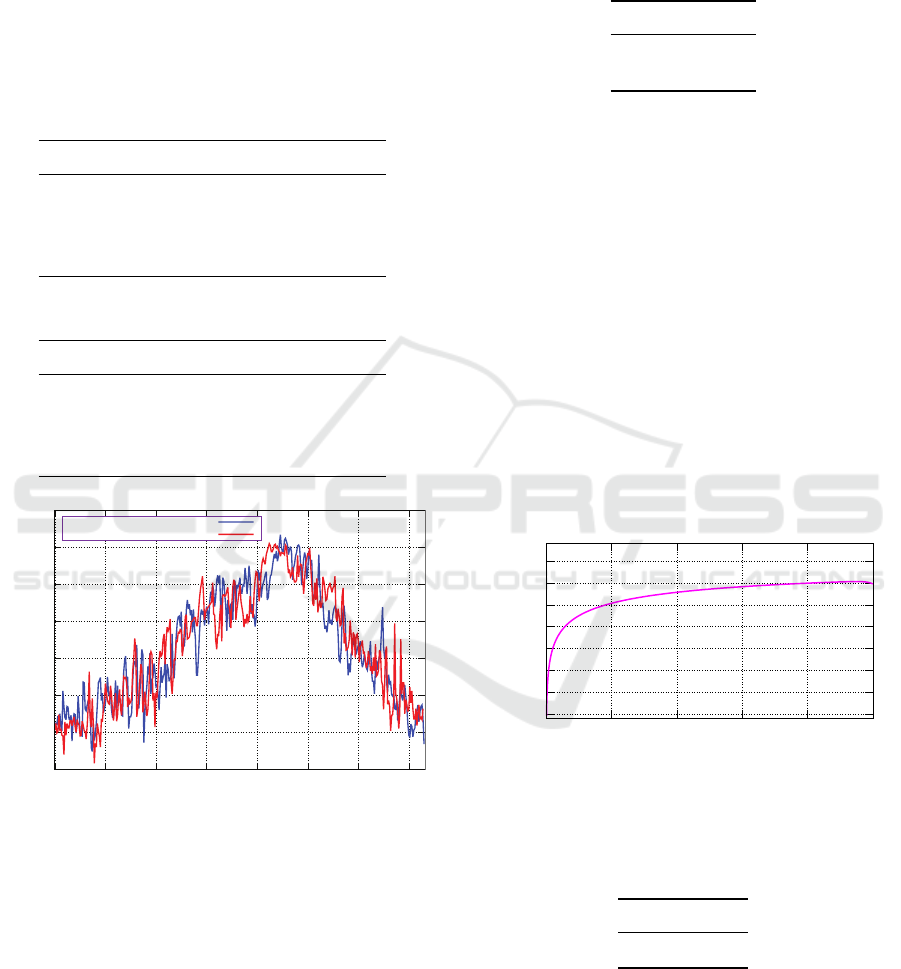
4.2 Data Specifications
Meteorological data is obtained as the daily average
temperature Celsius in Tokyo from January 1, 2019 to
December 31, 2020 (Japan Meteorological Agency,
2020). Table 1 and 2 show both training and test data
specifications. Figure 1 shows their time series plots.
In Figure 1, the red line shows time series of training
data and the blue line shows that of test data.
Table 1: Training Data Specifications.
Items Values
Monitoring Point: Tokyo
From: January 1, 2019
To: December 31, 2019
Total Days (t
max
): 365
Table 2: Test Data Specifications.
Items Values
Monitoring Point: Tokyo
From: January 1, 2020
To: December 31, 2020
Total Days (t
max
): 366
0
5
10
15
20
25
30
35
0 50 100 150 200 250 300 350
Temperature Celsius
days
Test Data (2020)
Training Data (2019)
Figure 1: Time Series Plots of Training and Test Data.
4.3 Initial Prior Distribution of
Parameter
According to both Definition 2.3 and Lemma 2.1, the
class of the prior distribution of parameter is gamma
distribution. If the non-informative prior (Berger,
1985; Bernardo and Smith, 2000) is considered un-
der gamma prior, it is the exactly same condition as
the author’s previous paper considering the nonsta-
tionary Poisson distribution (Koizumi, 2020, p. 999,
4.3). Therefore, the detail explanation is omitted and
the only hyperparameter settings in Definition 2.3 are
shown in Table 3.
Table 3: Defined Hyperparameters for Prior distribution
p(λ
1
).
Items Values
α
1
x
1
β
1
1
4.4 Results
4.4.1 Hyperparameter Estimation
For the approximate maximum likelihood estimator
of hyperparameter
ˆ
k in Eqs. (20) and (22), numeri-
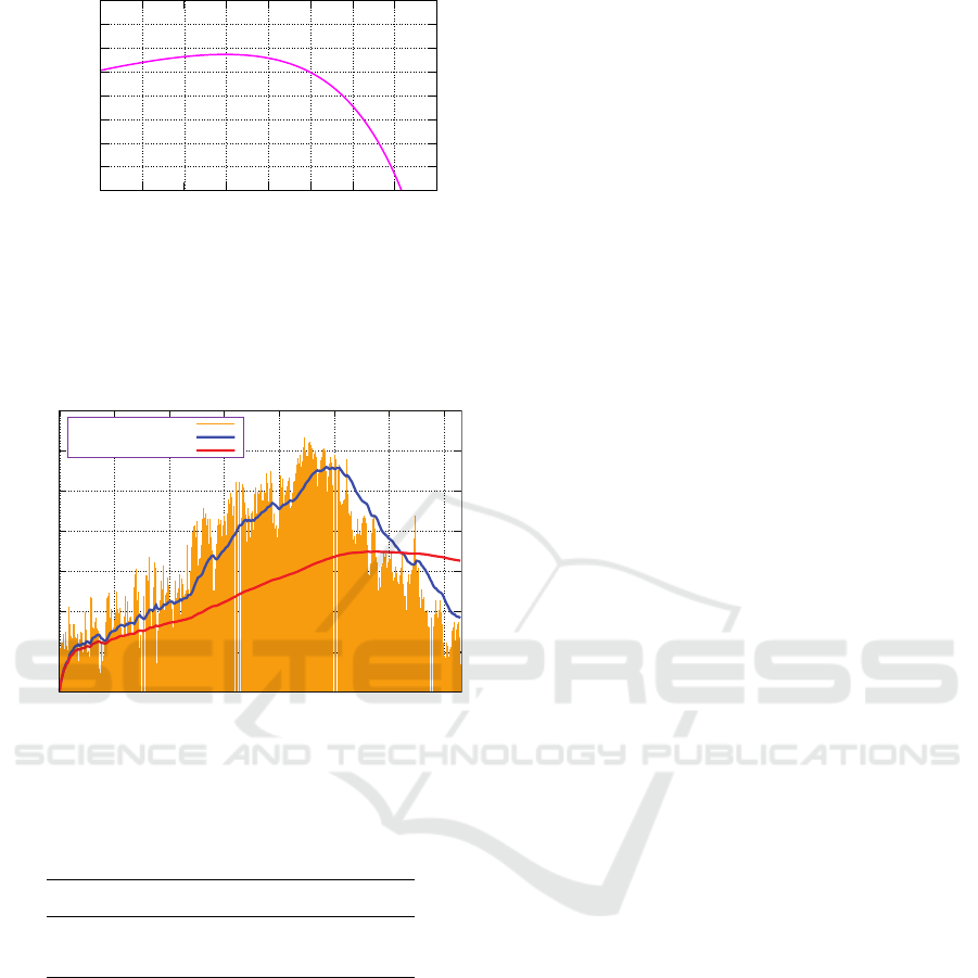
cal calculation is executed with training data. Fig-
ure 3 and 4 show the plot for loglikelihood function
logl (k) in Eq. (22). In Figure 2, the horizontal axis of
0 ≤ k ≤ 1 shows the range of k which is divided into
1,000 subintervals and the vertical axis shows value of
logl (k) in Eq. (22) with the logarithm base 10
3
which
is required to avoid the numerical underflow. Figure
3 shows similar plot with enlarged horizontal axis of
0.92 ≤ k ≤ 1.00. Finally, Table 4 shows the value of
ˆ
k.
-500
-450
-400
-350
-300
-250
-200
-150
0 0.2 0.4 0.6 0.8 1
Loglikelihood
k
Figure 2: Loglikelihood Function logl(k) with the Loga-
rithm Base 10
3
for 0 ≤ k ≤ 1.
Table 4: Hyperparameter Estimation Result from Training
Data.
Item Value
ˆ
k 0.950
4.4.2 Bayes Optimal Prediction
Figure 4 shows time series plot of the observed data
(orange bar), the prediction by the proposed model
(blue line), and the prediction by the stationary model
(red line) from test data. Table 5 shows the values
On the Prediction of a Nonstationary Exponential Distribution Based on Bayes Decision Theory
197

-200
-199.5
-199
-198.5
-198
-197.5
-197
-196.5
-196
0.92 0.93 0.94 0.95 0.96 0.97 0.98 0.99 1
Loglikelihood
k
Figure 3: Loglikelihood Function logl(k) with the Loga-
rithm Base 10
3
for 0.92 ≤ k ≤ 1.00.
of cumulative squared error in Definition 4.1 for pro-
posed and stationary models.
0
5
10
15
20
25
30
35
0 50 100 150 200 250 300 350
Temperature Celsius
days
Observed Values
Proposed
Stationary
Figure 4: Predictions of the Proposed and Stationary Mod-
els for Test Data.
Table 5: Cumulative Losses for the Proposed and Stationary
Models.
Items Cumulative Squared Error
Stationary 62.4
Proposed 12.8
5 DISCUSSIONS
The hyperparameter k in Eq. (2) generalizes a station-
ary exponential distribution to a nonstationary one.
If k = 1 in Eq. (2), then λ
t+1
= u
t
λ
t
holds. Conse-
quently, U
t
∼ Beta [α
t
,0] in Eq. (5). As the second
shape parameter in the beta distribution becomes zero,
the variance of u
t
becomes zero as well. This means
that the parameter λ
t
in the exponential distribution of
x
t
is stationary. However, if 0 < k < 1 in Eq. (2), then
λ
t
is nonstationary.
In Eqs. (8), β
t
is expressed by the term
∑
t−1
i=1
k
t−i
x
i
.
This form is called the Exponentially Weighted Mov-
ing Average (EWMA) (Smith, 1979, p. 382),(Harvey,
1989, p. 350), which has also been observed in sev-
eral versions of SPSMs (Smith, 1979; Koizumi, 2020;
Koizumi, 2021).
Regarding the hyperparameter estimation with
real data in 3.3, Figure 2 and 3 empirically show
that the likelihood function l (k) is upward convex in
0 ≤ k ≤ 1. Even if a numerical calculation is required,
the optimality of approximate maximum likelihood
estimator
ˆ
k in Eq. (20) is partially guaranteed.
Regarding the Bayes optimal prediction, Figure
4 demonstrates that the prediction values of the pro-
posed model follow a time series of test data more
closely than those of the stationary model. In fact,
Table 5 indicates that the value of the cumulative
squared error of the proposed model is approximately
twenty percent of that of the stationary model.
However, a more detailed analysis does not re-
veal that the proposed method is good prediction al-
gorithm. The heights of the orange bars in Figure
4 basically increase until the 224th day. In fact, the
highest daily average temperature is 31.7 [
◦
C] on the
224th day, namely, August 11th in summer, 2020 in
Tokyo. The blue line in Figure 4 also increases un-
til 224th day. However, the 117 proposed predictions
over 224 days, in other words 79.0%, are underes-
timated compared to the observed temperatures. On
the other hand, after 225th day, the heights of the or-
ange bars in Figure 4 start to decrease because the fall
or winter seasons approach. The 113 proposed pre-
dictions over the remaining 142 days, namely, 79.6%,
are overestimated compared to the observed temper-
atures. This result can be attributed to the fact that
the loss function based on the Bayes decision the-
ory is defined as the squared loss function stated in
Eq. (10). The squared loss function is quadratic, and
there is a significant predictive error if either overesti-
mation or underestimation errors occur. In summary,
the squared loss function yields the expectation of the
predictive distribution with the Bayes optimal predic-
tion, which often focuses on the middle range of ob-
served data. If one is not satisfied with the above sit-
uation, another loss function should be defined.
6 CONCLUSION
This paper considered a specific class of nonstation-
ary exponential distributions. We clarified that the
Bayes optimal prediction governed by both the non-
stationary distribution and squared loss function can
be obtained through simple arithmetic calculations if
the nonstationary hyperparameter is known. Using
ICAART 2023 - 15th International Conference on Agents and Artificial Intelligence
198

real meteorological data, the predictive performance
of the proposed algorithm was proven superior to that
of the stationary algorithm.
In the nonstationary hyperparameter estimation,
the approximate maximum likelihood estimation is
considered. We empirically observed that the likeli-
hood function has an upward convexity regarding spe-
cific data. The general convexity should be proven,
which is left for discussion in future research.
Moreover, the Bayes optimal prediction with loss
functions other than the squared loss should be con-
sidered, which is another future research topic.
REFERENCES
Allen, A. O. (1990). Probability, Statistics, and Queueing
Theory with Computer Science Applications (Second
Edition). Acaremic Press, San Diego.
Berger, J. (1985). Statistical Decision Theory and Bayesian
Analysis. Springer-Verlag, New York.
Bernardo, J. M. and Smith, A. F. (2000). Bayesian Theory.
John Wiley & Sons, Chichester.
Carlin, B. and Louis, T. (2000). Bayes and Empirical Bayes
Methods for Data Analysis (Second Edition). Chap-
man & Hall, New York.
Gnedenko, B. V., Belyayew, Y. K., and Solovyev, A. D.
(1969). Mathematical Methods of Reliability Theory.
Acaremic Press, New York.
Harvey, A. C. (1989). Forecasting, Structural Time Series
Models and the Kalman Filter. Cambridge University
Press, Marsa, Malta.
Hogg, R. V., McKean, J. W., and Craig, A. T. (2013). Intro-
duction to Mathematical Statistics (Seventh Edition).
Pearson Education, Boston.
Japan Meteorological Agency (2020). ClimatView
(in Japanese). https://www.data.jma.go.jp/gmd/cpd/
monitor/dailyview/. Browsing Date: Oct. 10, 2022.
Johnson, N. L., Kotz, S., and Balakrishnan, N. (1994). Con-
tinuous Univariate Distributions Volume 1 (Second
Edition). Willey & Sons, New York.
Kleinrock, L. (1975). Queueing Systems Volume I:Theory.
John Wiley & Sons, New York.
Koizumi, D. (2020). Credible interval prediction of a non-
stationary poisson distribution based on bayes deci-
sion theory. In Proceedings of the 12th Interna-
tional Conference on Agents and Artificial Intelli-
gence - Volume 2: ICAART, pages 995–1002. IN-
STICC, SciTePress.
Koizumi, D. (2021). On the prediction of a nonstation-
ary bernoulli distribution based on bayes decision the-
ory. In Proceedings of the 13th International Confer-
ence on Agents and Artificial Intelligence - Volume 2:
ICAART, pages 957–965. INSTICC, SciTePress.
Press, S. J. (2003). Subjective and Objective Bayesian
Statistics: Principles, Models, and Applications. John
Wiley & Sons, Hoboken.
Ross, S. (1997). Introduction to Probability Models (Sixth
Edition). Academic Press, San Diego.
Smith, J. Q. (1979). A generalization of the bayesian steady
forecasting model. Journal of the Royal Statistical So-
ciety - Series B, 41:375–387.
Trivedi, K. S. (1982). Probability & Statistics with Reli-
ability, Queuing and Computer Science Applications.
Prentice-Hall, Englewood Cliffs.
APPENDIX
A: Proof of Lemma 2.1
Note that time index t has been omitted for simplicity;
for example, λ
t
is written as λ, x
t
is written as x, and
so on. Suppose that data x are observed under the
parameter λ following Eq. (2). Then, according to
the Bayes theorem, the posterior distribution of the
parameter p

λ


x

is as follows:
p

λ


x

=
p

x


λ

p

λ


α,β


+∞
0
p

x


λ

p

λ


α,β

dλ
=
β
α
Γ(α)
(λ)
α−1
exp[−(β + x)λ]
β
α
Γ(α)

+∞
0
(λ)
α−1
exp[−(β + x)λ]dλ
=
(λ)
α−1
exp[−(β + x)λ]

+
∞
0
(λ)
α
−
1
exp[−(β + x)λ]dλ
. (24)
Then the denominator of the right-hand side in Eq.
(24) becomes,

+∞
0
(λ)
α−1
exp[−(β + x)λ]dλ =
Γ(α + 1)
(β + x)
α+1
. (25)
Note that Eq. (25) is obtained by applying the fol-
lowing property of the gamma function.
Γ(x)
q
x
=

+∞
0
y
x−1
exp(−qy)dy . (26)
Substituting Eq. (25) in Eq. (24),
p

λ


x

=
(β + x)
α+1
Γ(α + 1)
(λ)
α−1
exp[−(β + x)λ]. (27)
Eq. (27) shows that the posterior distribution of
the parameter p

λ


x

also follows the gamma distri-
bution with parameters α+ 1,β +x, which is the same
class of distribution as Eq. (3). This is the nature of
the conjugate family (Bernardo and Smith, 2000) for
exponential distribution.
Suppose the nonstationary transformation of the
parameter λ in Eq. (2). Similar transformation of pa-
rameters for the beta distribution is discussed (Hogg
On the Prediction of a Nonstationary Exponential Distribution Based on Bayes Decision Theory
199

et al., 2013, pp. 162–163). According to Definition
2.6, the joint distribution p(λ,u) is the product of the
probability distributions of λ in Eq. (3) and u in Eq.
(5),
p(λ, u) = p(λ) p(u)
=
(β)
α
Γ(kα)Γ [(1 − k)α]
(u)
kα−1
·(1 − u)
(1−k)α−1
(λ)
α−1
exp(−βλ).(28)
Denote the two transformations as



v =
λu
k
;
w =
λ(1−u)
k
,
(29)
where λ > 0, 0 < u < 1, and 0 < k ≤ 1.
The inverse transformation of Eq. (29) becomes



λ = k (v + w) ;
u =
v
v+w
.
(30)
The Jacobian of Eq. (30) is
J =






∂λ
∂v
∂λ
∂w
∂u
∂
v
∂u
∂
w






=






k k
w
(v+w)
2
−
v
(v+w)
2






(31)
= −
k
v + w
= −
k
2
λ
̸= 0. (32)
The transformed joint distribution p(v, w) is ob-
tained by substituting Eq. (30) for (28), and multi-
plying the right-hand side of Eq. (28) by the absolute
value of Eq. (31):
p(v, w)
=
(β)
α
Γ(kα)Γ [(1 − k)α]

v
v + w

kα−1
·

w
v + w

(1−k)α−1
[k (v + w)]
α−1
·exp [−kβ(v + w)] ·



−
k
v + w



=
(kβ)
α
Γ(kα)Γ [(1 − k)α]
(v)
kα−1
(w)
(1−k)α−1
·
exp
[
−
k
β
(
v
+
w
)]
.
(33)
Then, p (v) is obtained by marginalizing Eq. (33),
p(v) =

+
∞
0
p(v, w)dw
=
(kβ)
α
(v)
kα−1
exp(−kβv)
Γ(kα)Γ [(1 − k)α]
·

+∞
0
(w)
(1−k)α−1
exp(−kβw) dw
=
(kβ)
α
(v)
kα−1
exp(−kβv)
Γ(kα)Γ [(1 − k)α]
Γ[(1 − k) α]
(kβ)
(1−k)α
=
(kβ)
kα
Γ(kα)
(v)
kα−1
exp(−kβv) . (34)
Eq. (34) is obtained by applying the property of
gamma function in Eq. (26).
According to Eq. (34), v follows the gamma dis-
tribution with parameters kα, kβ.
Considering two Eqs. (27) and (34), it has been
proven that if the prior distribution of the scale param-
eter satisfies Λ ∼ Gamma(α, β), then its transformed
posterior distribution satisfies,
Λ


x ∼ Gamma[k (α + 1), k (β + x)] . (35)
By adding the omitted time index t, the recursive
relationships of the parameters of the gamma distri-
bution can be formulated as,

α
t+1
= k (α
t
+ 1);
β
t+1
= k (β
t
+ x
t
).
(36)
Thus, for t ≥ 2, the general α
t
,β
t
in terms of the
initial α
1
,β
1
can be written as,







α
t
= k
t−1
α
1
+
t−1
∑
i=1
k
i
;
β
t
= k
t−1
β
1
+
t−1
∑
i=1
k
t−i
x
i
.
(37)
This completes the proof of Lemma 2.1. 
ICAART 2023 - 15th International Conference on Agents and Artificial Intelligence
200

B: Proof of Lemma 2.2
From Eqs. (1) and (7), the predictive distribution un-
der observation sequence x
x
x
t
becomes,
p

x
t+1


x
x
x
t

=

+∞
0
p

x
t+1


λ
t+1

p

λ
t+1


x
x
x
t

dλ
t+1
(38)
=

+∞
0
[λ
t+1
exp(−λ
t+1
x
t+1
)]
·

(β
t+1
)
α
t+1
Γ(α
t+1
)
(λ
t+1
)
α
t+1
−1
exp(−β
t+1
λ
t+1
)

dλ
t+1
(39)
=
(β
t+1
)
α
t+1
Γ(α
t+1
)
·

+∞
0
(λ
t+1
)
α
t+1
exp[−(β
t+1
+ x
t+1
)λ
t+1
]dλ
t+1
(40)
=
(β
t+1
)
α
t+1
Γ(α
t+1
)
Γ(α
t+1
+ 1)
(β
t+1
+ x
t+1
)
α
t+1
+1
(41)
=
Γ(α
t+1
+ 1)(β
t+1
)
α
t+1
Γ(α
t+1
)(β
t+1
+ x
t+1
)
α
t+1
+1
(42)
Note that Eq. (41) is obtained by applying the prop-
erty of gamma function in Eq. (26).
This completes the proof of Lemma 2.2. 
On the Prediction of a Nonstationary Exponential Distribution Based on Bayes Decision Theory
201