Explainable Outlier Detection Using Feature Ranking for k-Nearest

Neighbors, Gaussian Mixture Model and Autoencoders

Lucas Krenmayr

and Markus Goldstein

Department of Computer Science, Ulm University of Applied Sciences, Prittwitzstraße 10, 89075 Ulm, Germany

Keywords:

Outlier Detection, Explainability, Anomaly Detection, k-NN, Gaussian Mixture Model, GMM, Autoencoder.

Abstract:

Outlier detection is the process of detecting individual data points that deviate markedly from the majority

of the data. Typical applications include intrusion detection and fraud detection. In comparison to the well-

known classiﬁcation tasks in machine learning, commonly unsupervised learning techniques with unlabeled

data are used in outlier detection. Recent algorithms mainly focus on detecting the outliers, but do not provide

any insights what caused the outlierness. Therefore, this paper presents two model-dependent approaches to

provide explainability in multivariate outlier detection using feature ranking. The approaches are based on the

k-nearest neighbors and Gaussian Mixture Model algorithm. In addition, these approaches are compared to

an existing method based on an autoencoder neural network. For a qualitative evaluation and to illustrate the

strengths and weaknesses of each method, they are applied to one synthetically generated and two real-world

data sets. The results show that all methods can identify the most relevant features in synthetic and real-world

data. It is also found that the explainability depends on the model being used: The Gaussian Mixture Model

shows its strength in explaining outliers caused by not following feature correlations. The k-nearest neighbors

and autoencoder approaches are more general and suitable for data that does not follow a Gaussian distribution.

1 INTRODUCTION

Outlier detection was ﬁrst introduced in the late 60s in

order to detect and often remove possible incorrect in-

stances from a data set. Grubbs (1969) was the ﬁrst to

introduce the term outlier and he also deﬁned it as an

outlying observation that appears to deviate markedly

from other members of the sample in which it occurs.

Today, the reason for performing outlier detection

is very different: The goal is mainly to identify the

outliers or anomalies in the data, since they can be

of great interest in various application scenarios. For

example, in intrusion detection, attackers or compro-

mised machines in computer networks can be found.

When applied on ﬁnancial or transaction data, fraudu-

lent records such as credit card fraud can be identiﬁed.

Sometimes, outlier detection is also called anomaly

detection, novelty detection, or has a speciﬁc name

based on the application scenario (fraud detection, in-

trusion detection).

Furthermore, outlier detection can be performed

in a supervised, a semi-supervised or an unsupervised

setting. The latter is by far the most relevant scenario

since outliers are often not available for training in ad-

https://orcid.org/0000-0002-6502-9133

https://orcid.org/0000-0003-2631-6882

vance. This paper focuses on an unsupervised setting

and algorithms thereof. In this context, it is also im-

portant to know that most of the modern unsupervised

outlier detection algorithms do not output a binary la-

bel, but an outlier score instead, indicating by how

much an instance is considered to be an outlier. In

practical applications, the scores are of great interest

because outliers can be ordered by their degree of out-

lierness and most interesting ones can be investigated

ﬁrst (Goldstein and Uchida, 2016).

Especially in multivariate outlier detection, the

subsequent analysis of the outliers poses a challeng-

ing task. In machine learning, the topic of explain-

ability has recently gained a lot of interest. In our

context of outlier detection, explainability has often

been tackled in the context of application domains,

but barely in a generic fashion (Panjei et al., 2022).

Modern outlier detection algorithms often use ma-

chine learning techniques (Aggarwal, 2017) and can

be categorized based on their underlying concept be-

ing used. Common are distance-based approaches

that use the assumption that normal data instances oc-

cur in dense neighborhoods, while outliers occur far

from their closest neighbors (Chandola et al., 2009).

A prominent approach in this area is the k-nearest

neighbors (k-NN) algorithm.

Krenmayr, L. and Goldstein, M.

Explainable Outlier Detection Using Feature Ranking for k-Nearest Neighbors, Gaussian Mixture Model and Autoencoders.

DOI: 10.5220/0011631900003411

In Proceedings of the 12th International Conference on Pattern Recognition Applications and Methods (ICPRAM 2023), pages 245-253

ISBN: 978-989-758-626-2; ISSN: 2184-4313

 2023 by SCITEPRESS – Science and Technology Publications, Lda. Under CC license (CC BY-NC-ND 4.0)

245

Other approaches are based on probabilities and

assume that normal data can be represented as a

stochastic model. The underlying principle of these

statistical-based outlier detection techniques is that

an outlier is an observation that is suspected of be-

ing partially or totally incorrect because it is not gen-

erated by the stochastic model assumed (Anscombe,

1960; Chandola et al., 2009). Statistical-based algo-

rithms ﬁt a model using the given data ﬁrst and then

apply a statistical inference test to determine whether

or not an instance belongs to that model. Instances

that have a low probability of being generated by the

learned model are considered as outliers. A promi-

nent approach here is the Gaussian Mixture Model

(GMM), which represents the underlying data distri-

bution with a ﬁxed number of Gaussian distributions

(called components).

Besides the two groups, Chandola et al. (2009)

further categorizes outlier detection algorithms into

clustering-based and classiﬁcation-based. The latter

category also contains autoencoder neural networks,

which will be used in this work as a third algorithm.

All of the categories have today in common that state-

of-the-art algorithms focus on detecting the outliers

and do not provide insights about what led to the out-

lier decision. These insights often have to be deter-

mined by experts manually by analyzing the outliers

in order to determine their root cause. In practice, this

is often a challenging task since the causes of outliers

are complex and even often hidden in multiple di-

mensions. Furthermore, detailed domain knowledge

is often required by the experts. Therefore, this pa-

per proposes a method for providing explainability of

the k-NN and GMM algorithms for outlier detection.

The basic idea is to rank each individual dimension

depending on its inﬂuence on the detected outliers by

analyzing the distances per dimension based on the

learned model. The goal is to support the experts

while analyzing the outliers by presenting the dimen-

sions that need to be examined more closely in order

to identify the cause or causes of the outlier.

2 RELATED WORK

2.1 k-Nearest Neighbors Outlier

Detection Algorithm

The global k-NN approach, often simply referred to as

k-NN, is a distance-based outlier detection approach

that uses the assumption that outliers occur far away

from their closest neighbors in comparison to nor-

mal instances. As described by Goldstein and Uchida

(2016), this approach detects outliers by ﬁrst calcu-

lating the k nearest neighbors for every data point in

the data set. Afterwards, the outlier score is computed

by either using the distance to the k

nearest neigh-

bor (a single one) (Ramaswamy et al., 2000) or the

average distance to all k nearest neighbors (Angiulli

and Pizzuti, 2002). The second approach is used

in the following. Here, the average Euclidean dis-

tance for a given point q to the k-nearest neighbors set

N = {n

,...n

} is calculated in the d-dimensional

space:

dist(q,N) = 1/k

∑

j=1

∑

i=1

− n

)

(1)

The choice of the parameter k is crucial for the results.

If it is too small, the local density estimate might not

be reliable. On the other hand, the density estimate

may be too coarse and thus outliers not found if it is

selected too large.

Several publications exist, in which this approach

is used for outlier detection. Amer and Goldstein

(2012) evaluated different distance-based outlier de-

tection approaches including k-NN for anomaly de-

tection on three different data sets. The authors found

that this approach performs especially well in detect-

ing global outliers.

2.2 Using a Gaussian Mixture Model

for Outlier Detection

A mixture model is a collection of probability distri-

butions or densities C

,... ,C

and mixing weights or

proportions w

,. .. ,w

, where k is the number of com-

ponent distributions (Lindsay, 1995; McLachlan and

Peel, 2000).

Therefore, the mixture model P is a probability dis-

tribution of the data based on a mixture of multiple

component distributions and their corresponding mix-

ing weights and is given as (Baxter, 2017):

P(x|C

,. .. ,C

,. .. ,w

) =

∑

j=1

P(x|C

) (2)

For the GMM, the probability distribution C is given

by the Gaussian distribution C = N (µ, σ

) in the one-

dimensional case with a mean of µ and variance of

In the multidimensional case, C is given by the

multivariate Gaussian distribution C = N (µ, Σ) with

a mean vector of µ and the covariance matrix of Σ.

P(x|θ) =

∑

j=1

P(x|N (µ, Σ)

) (3)

To estimate the parameters θ = (w,µ, Σ) of the compo-

nents, the expectation maximization (EM) algorithm

ICPRAM 2023 - 12th International Conference on Pattern Recognition Applications and Methods

246

introduced by Dempster et al. (1977) is applied. This

algorithm aims to estimate the parameters θ in such

a way that they maximize the joint probability of the

data set by solving the following optimization prob-

lem:

argmax

P(X|θ) = argmax

∏

P(x

|θ)

= argmax

∏

(

∑

j=1

P(x

|N (µ

, Σ

)) (4)

In practice, GMMs are used in several unsuper-

vised learning setups, e.g., density estimation, model-

based clustering and outlier detection. In the latter,

the estimated likelihood or, due to computational rea-

sons, the log-likelihood per data point is then used as

an outlier score.

2.3 Autoencoder for Outlier Detection

An autoencoder (AE) is a neural network trained in a

speciﬁc way in order to learn reconstructions that ap-

proximate the original input (Goodfellow et al., 2016,

p.499). An AE consists of two parts, an encoder and a

decoder part. An AE with a single hidden layer could

be represented by the following equations, where w, ˆw

and b,

b are the weights and biases of the encoder and

decoder and σ,

σ are the activation functions (An and

Cho, 2015):

h = σ(wx + b) (5)

ˆx =

σ( ˆwh +

b) (6)

MAE =

∑

i=1

− ˆx

| or MSE =

∑

i=1

− ˆx

)

(7)

Equation 5 describes the encoder step, mapping an in-

put vector x to a hidden representation h by an afﬁne

mapping following an activation function. Equation 6

shows the decoder step, reconstructing the hidden rep-

resentation h back to the original input space by the

same transformation as the encoder. The difference

between the input vector x and the reconstructed out-

put ˆx in the d dimensional space, described in Equa-

tion 7, is called the reconstruction error. As a metric,

the mean absolute error (MAE) or the mean squared

error (MSE) is often used to calculate the reconstruc-

tion error. During the training, the AE learns to min-

imize the reconstruction error by using backpropaga-

tion and stochastic gradient descent.

Due to the usage of a non-linear activation function,

the AE is capable of learning non-linear relationships.

Using the hidden representation of an AE as an in-

put to another one makes it possible to stack AEs,

also known as deep autoencoder. To force a com-

pressed representation in the hidden layers, the num-

ber of units in the hidden layers is subsequently re-

duced. This introduces a bottleneck that forces the AE

to learn the most relevant features and relationships of

the data. Hawkins et al. (2002) ﬁrst used this concept

for the task of outlier detection. The key idea is that

during training, the weights of the AE are adjusted to

minimize the reconstruction error for all training pat-

terns. As a result, frequent patterns are more likely

to be well reproduced by the trained AE, so the pat-

terns that represent outliers are less well reproduced

and have a higher reconstruction error. The recon-

struction error is then used as the outlier score.

2.4 Explainability in Outlier Detection

To understand explainability within the context of

outlier detection, ﬁrst a deﬁnition in the wider area of

artiﬁcial intelligence (AI) is reviewed. Explainabil-

ity in AI (XAI) refers to the concept of being able to

understand the machine learning model. This is of-

ten crucial since the underlying machine learning al-

gorithms construct complex models which are often

opaque to humans (Burkart and Huber, 2020) and ap-

pear as black box models. It is important to stress

that it aims to explain causal effects in the model and

not casual effects in the domain (Herskind Sejr et al.,

2021). The focus towards XAI is currently in the con-

text of supervised learning. However, also in the ﬁeld

of unsupervised learning, the principles of XAI are

applicable. We believe that the widespread applica-

tion of unsupervised outlier detection in practice is

still behind due to missing conﬁdence and trust. In

particular, the algorithms lack of association between

detected outliers and their root causes. This is espe-

cially relevant for multivariate outlier detection: Here,

outliers are often complex situations, where causes

are hidden in multiple dimensions. It is difﬁcult to

identify them without additional insights.

Explainability in outlier detection has just recently

gained importance. In comparison to other sub-areas

of AI, only limited work on this topic is available.

However, a summary of the current state of this topic

is provided by Panjei et al. (2022) and Sejr and

Schneider-Kamp, who refer to the topic of explain-

able outlier detection with the term XOD.

In this work, we present two approaches that pro-

vide a weight vector as output, which can be inter-

preted as feature ranking and is intended to provide

an explanation of which features are most important

according to the used outlier detection algorithm.

Explainable Outlier Detection Using Feature Ranking for k-Nearest Neighbors, Gaussian Mixture Model and Autoencoders

247

3 EXPLAINABLE OUTLIER

DETECTION

3.1 Explainable k-Nearest Neighbors

Outlier Detection

For the k-NN approach, we propose an outlier expla-

nation by ranking individual dimensions accordingly

to how strongly they contribute to the detected outlier.

This is achieved by computing the average Euclidean

distance per dimension d for an outlier point q to the

k-nearest neighbors set N as described in Equation 8:

dist

(q,N) =

∑

j=1



− n



∀d (8)

As it is well-known for k-NN outlier detection, the

results of the described dimensional ranking are

strongly dependent on the parameter k.

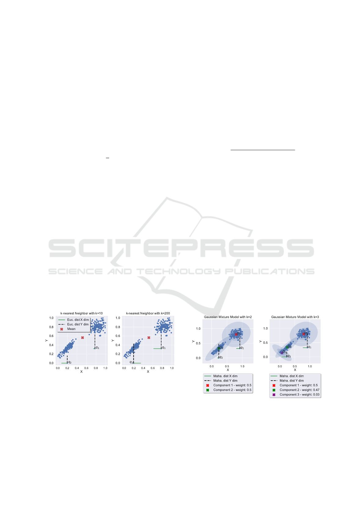
Figure 1 shows the outcome for different values of

k in a two-dimensional space. Here, the solid green

and dashed black lines visualize the mean distance of

the X and Y dimension of two selected outliers q

and

. On the left-hand side, it can be seen how this ap-

proach behaves for small values of k. Dimensions that

have large deviations to the nearest, more dense area

result in a larger distance. This indicates which di-

mension would have to be shifted to get to a more

dense area (e.g. causing the outlier). However, on

the right-hand side, it can be seen that the average

distance per dimension approaches the global average

indicated by the red dot for large values of k.

This approach is later used to assess the inﬂuence

per dimension on the outlier and therefore to provide

an explanation of why a particular instance was de-

tected as an outlier.

Figure 1: Feature ranking: Mean Euclidean distance per

dimension for two selected outliers with k = 10 (left) and a

too large value of k = 200 (right).

3.2 Explainable Gaussian Mixture

Model Outlier Detection

To enable explanations for the GMM model, also a

ranking of individual dimensions accordingly to how

strongly they contribute to the outlier is proposed.

Since the data is described by a ﬁnite set of Gaus-

sian components, the Mahalanobis distance is used.

Therefore, for an outlier q, the vector ⃗m is calculated,

representing the Mahalanobis distances for each di-

mension to the best ﬁtting component C (cf. Equa-

tion 9). This is obtained by replacing the dot prod-

uct of the Mahalanobis distances equation with the

element-wise product. From the resulting vector, the

element-wise absolute values are taken to eliminate

negative values. C is chosen based on which compo-

nent maximizes the log-likelihood for the data point

⃗m =

|(q − µ

)

⊤

−1

◦ (q − µ

)| (9)

An example of how this feature ranking behaves on a

data set generated from two Gaussian distributions is

visualized in Figure 2. On the left, the Mahalanobis

distance per dimension of the outliers q

to the best

ﬁtting component C

, and q

to the component C

presented for the X and Y dimension. A GMM with

k = 2 is ﬁtted to the data. Both outliers show a larger

Mahalanobis distance on the Y dimension than on the

X dimension. This is because they are both close to

the mean of their best ﬁtting component on the X di-

mension. However, on the Y dimension, they are both

off. Therefore, this is used as an indication that the Y

dimension is mainly causing the outlier. Also, the out-

lier q

shows a larger Mahalanobis distance on the Y

dimension than q

, even though the difference on this

dimension to the mean of the best ﬁtting component

is larger for q

. This presents the difference of the

Mahalanobis distance in comparison to the Euclidean

distance. It also considers the variance per dimension

and thus results in a larger distance of q

to C

dimension Y in comparison to q

to C

Figure 2: Mahalanobis distance per dimension for two se-

lected outliers as explanation. On the left a GMM with k = 2

and on the right a GMM with k = 3 is ﬁtted on the data.

ICPRAM 2023 - 12th International Conference on Pattern Recognition Applications and Methods

248

This approach is again highly dependent on the

parameter k of the GMM. When choosing k to large,

the GMM tends to learn low-weighted components

which describe the outliers.This is contrary to the idea

of using the best-ﬁtting components, since here the

best-ﬁtting component is distorted by the outlier. The

right plot visualizes this behavior where a GMM with

k = 3 is ﬁtted on the data, whereas the low-weighted

component C

with a weight factor of w = 0.03 is dis-

torted due to the outlier q

. To avoid such a situation,

the parameter k should be chosen large enough to suf-

ﬁciently describe the normal data but low enough to

prevent overﬁtting on the outliers. Another solution

could also be to ignore low-weighted components.

3.3 Explainable Outlier Detection for

Autoencoders

To explain how much each dimension contributed to

the detected outlier using an AE, the reconstruction

error per dimension between the input vector x and

the reconstructed output ˆx is used. The assumption is,

that in case certain dimensions show a higher recon-

struction error than other dimensions, they are more

likely to deviate from their usual distribution. This

idea was introduced by Antwarg et al. (2019) using a

similar approach for explaining the outcome of an AE

for anomaly detection.

4 EVALUATING EXPLAINABLE

OUTLIER DETECTION

ALGORITHMS

To assess the effectiveness and compare the outcomes

of the presented approaches, an evaluation using a

synthetically generated data set and two real-world

data sets Wine Quality and KDD-HTTP-Cup are used.

The source code for this evaluation is publicly avail-

able on GitHub

. Although outlier detection is done

in practice using unsupervised learning, the hyperpa-

rameters per data set are listed in Table 1 and were

selected by hyperparameter tuning based on the max-

imization of the AUC of the ROC curve. This was

done to ensure that the selected methods are suitable

for outlier detection on the used datasets in the ﬁrst

place. Since the focus of this work is on how these ap-

proaches are explaining outliers, it requires that out-

liers are detected reliably. Furthermore, only true pos-

itive detected outliers were used for further analysis.

github.com/lucas8k/explainable outlier detection

Table 1: Hyperparameters for the approaches applied on the

synthetic, wine quality and KDD-Cup99 data set.

Approach Hyperparameter

Values

(Synthetic)

Values

(Wine quality)

Values

(KDD-Cup99)

Gaussian Mixture Model Components 2 3 3

k-Nearest Neighbors k 10 43 50

Autoencoder

Encoder Dimensions

Decoder Dimensions

Activation Function

Hidden Layer

Activation function

Output Layer

Learning Rate

Epochs

Batch Size

6-4-2

2-4-6

tanh

Sigmoid

1e-3

11-9-7-5

5-7-8-11

tanh

Sigmoid

1e-3

100

29-25-22-20

20-22-25-29

tanh

Sigmoid

1e-3

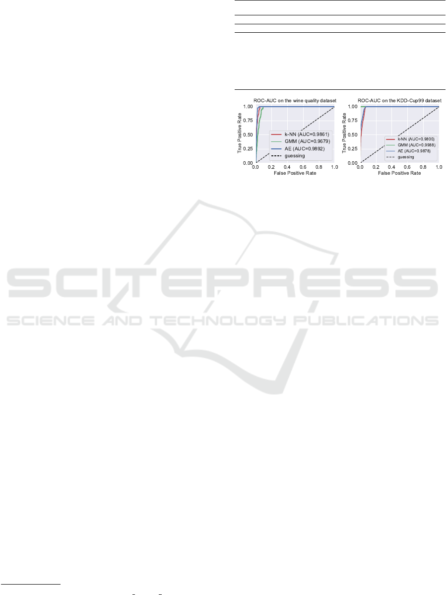
Figure 3: ROC-AUC of the different methods on the wine

quality data set (left) and the KDD-Cup99 data set (right).

4.1 Synthetic Data Set

The synthetic data set consists of 2,000 6-dimensional

data points sampled from two Gaussian distributions

(µ

, Σ

) and N

(µ

, Σ

) where the elements of the

vector µ

are all set to 0 and for the covariance matrix

the diagonal is set to 1 and all other elements are

set to 0.9. The elements of the vector µ

are all set

to 12 and for the covariance matrix µ

the diagonal is

set to 1 and all other elements are set to 0.3. Then,

the four outliers q

... q

were introduced by shifting

the point in the ﬁrst two dimensions while keeping the

last four dimensions The resulting data set is visual-

ized in Figure 4. Here it can clearly be seen that the

data set consists of two clusters and the four outliers

are only observable in the projection of the ﬁrst two

dimensions.

The methods presented are applied to the synthetic

data set. Afterwards, the feature ranking of the out-

liers are calculated. For a better comparison, the re-

sults are scaled into a common interval of [0, 1]. The

feature rankings are visualized in Figure 5. It can be

seen that all three approaches identiﬁed either the ﬁrst

dimension (D1), the second dimension (D2) or both

as important for detecting the outlier.

In addition to identify the important features, the

feature ranking can also be interpreted as a distance

per dimension. This provides information about the

direction in which the point would have to be moved

to reduce the outlier score. For example, in Figure 6

the outlier q

including the feature ranking given by

the different approaches is visualized in the dimen-

sions D1 and D2. On the left, the distance to the k

Explainable Outlier Detection Using Feature Ranking for k-Nearest Neighbors, Gaussian Mixture Model and Autoencoders

249

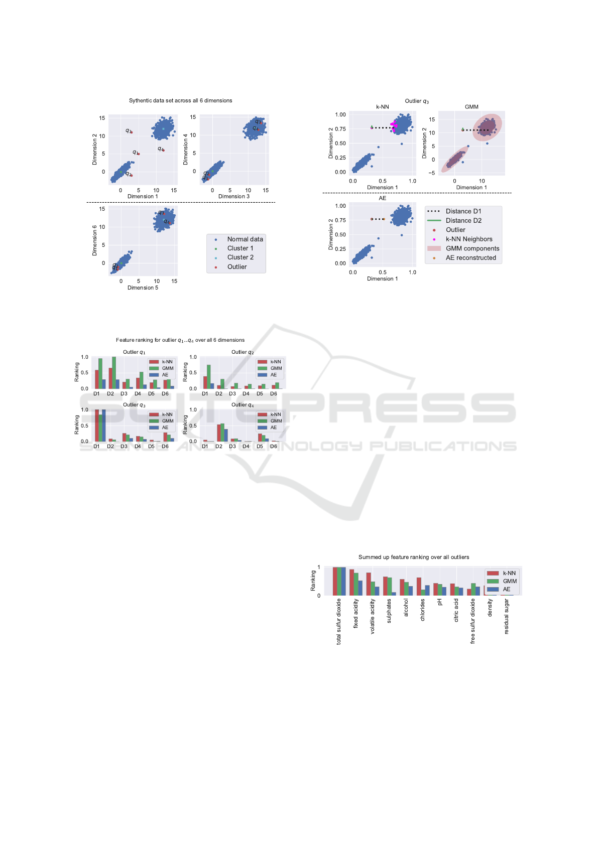
Figure 4: Synthetic data set consisting of 2,000 6-

dimensional data points sampled from two Gaussian distri-

butions including four outliers in the ﬁrst two dimensions.

Figure 5: Feature ranking of the introduced outliers over

all 6-dimensions for the three approaches scaled into the

common range of [0,1].

nearest neighbors is visualized. In the middle, the

Mahalanobis distance to the component C1 is visu-

alized. On the right, the difference between the re-

constructed and actual data points is visualized. All

three approaches report the D1 dimension as the most

important feature. Overall, the experiments with the

synthetic data set show, that all three presented ap-

proaches are capable of detecting the relevant dimen-

sions for explaining the causes of the outliers.

4.2 Wine Quality Data Set

As a ﬁrst real-world data set, a modiﬁed version of the

wine quality UCI data set (Cortez et al., 2009) is used.

The data set describes the physicochemical properties

of the red and white variants of the Portuguese ”Vinho

Verde” wine by 11 continuous features. Initially, the

data set was collected for classiﬁcation or regression

tasks. For the task of outlier detection, the data set

Figure 6: Feature Ranking for the dimensions D1 and D2

for the outlier q

. The outlier is mainly caused by D1.

was modiﬁed: The class white wine is used as the

normal class. The class red wine is down-sampled to

50 instances representing the outliers. This results in

a data set containing 4821 normal instances and 50

outliers with an outlier rate of approx. 1.03%.

The presented algorithms are also applied on this data

set. All three approaches achieved an AUC-ROC

of over 96% as visualized in Figure 3 (left). This

means, overall the approaches are suitable to detect

the outliers. Therefore, the presented explainability

approaches are applied to explain the outliers using

feature ranking. For every approach, ﬁrst the rele-

vant features of the data set causing outliers are iden-

tiﬁed. For this purpose, the feature ranking for all

three approaches across all outliers are summed up,

and scaled into a common range of [0,1]. The results

are visualized in Figure 7. As can be observed all

three approaches detect the feature total sulfur diox-

ide as the most relevant followed by the features ﬁxed

acidity, volatile acidity and sulphates.

Figure 7: Wine Quality data set: Summed-up feature rank-

ing of the outliers (red wine) over all 6-dimensions for the

three approaches scaled into the common range of [0,1].

Recalling the insights from the experiment, these

features are the root causes and should be most impor-

tant for identifying the outliers (red wine) within the

ICPRAM 2023 - 12th International Conference on Pattern Recognition Applications and Methods

250

normal instances. Therefore, we try to verify the re-

sults by additionally using the class labels of the data

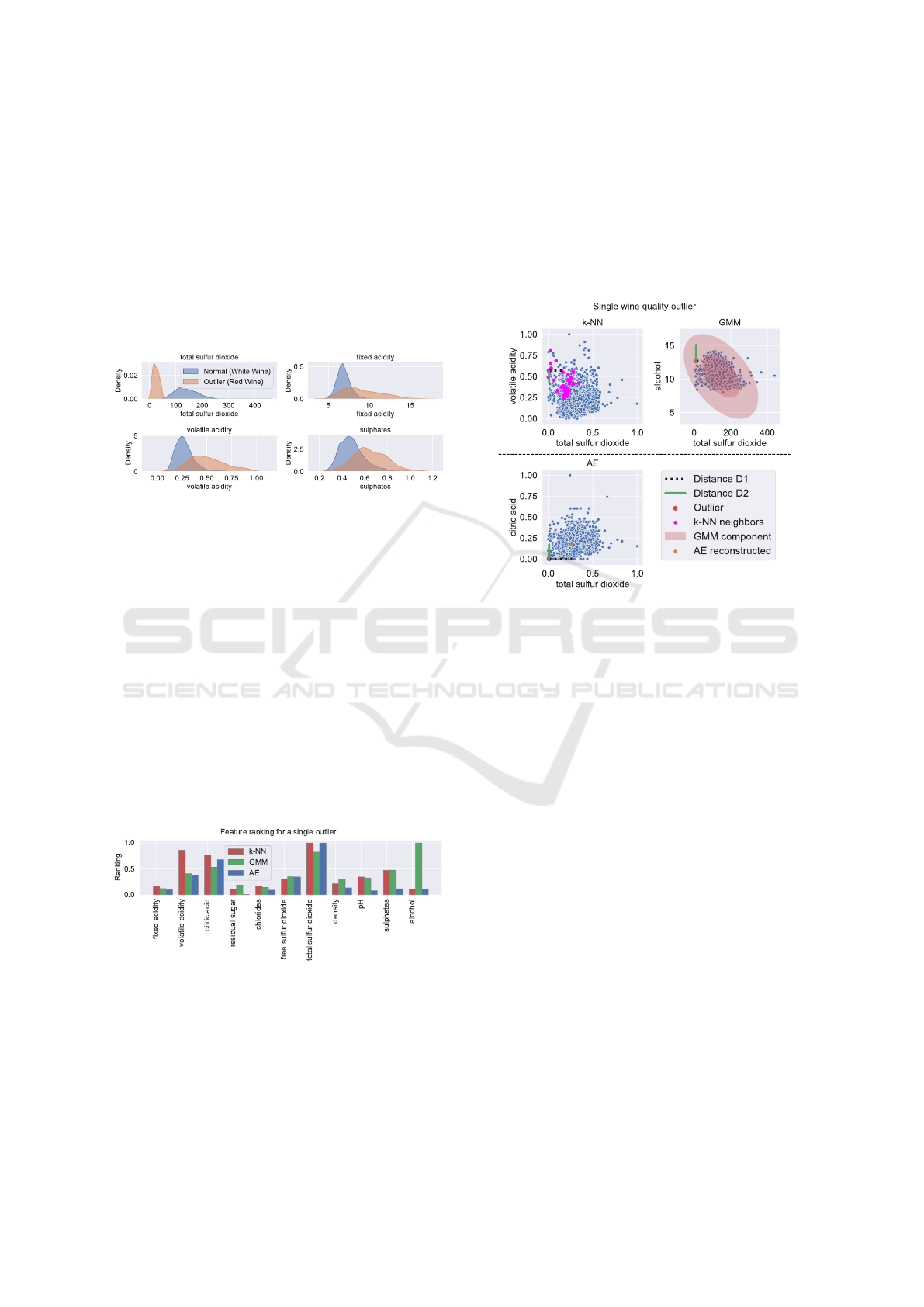
set in a plot. Figure 8 visualizes the density estima-

tion of the outlier (red wine) and regular (white wine)

for the top four features. It can be seen that especially

the feature total sulfur dioxide clearly separates the

outlier and normal instances. The other three features

also show large areas of non-overlap in the density es-

timation, but there is also certain overlap where these

features are not sufﬁcient to distinguish between out-

liers and normal instances.

Figure 8: Density estimation for the top 4 features for the

outliers (red wine) and normal instances (white wine).

Additionally, the feature ranking is also suitable

for analyzing and explaining single outliers. As

shown in Figure 7, the feature total sulfur dioxide

is the most dominant features overall. However,

when analyzing individual outliers, it can be seen

that in a few cases there are differences in what the

second most important features is, depending on the

approach chosen. In concrete terms, this behavior

can be observed for outliers, such as the one shown in

Figure 9. Here, the feature ranking is visualized for a

single outlier. It can be seen that the k-NN approach

considers the feature volatile acidity and the AE

the feature citric acid as the second most important

feature (cause). The GMM approach even ranks the

feature alcohol above the feature total sulfur dioxide.

Figure 9: Wine Quality data set: Feature ranking for a single

outlier over all 6-dimensions for the three approaches scaled

into the common range of [0,1].

This shows that the feature ranking is model de-

pendent and therefore does not provide a general ex-

planation. An example of this is visualized in Fig-

ure 10. Here we can see that both, the AE and k-

NN approaches, rank the features with the largest Eu-

clidean distance the highest. The correlation between

certain features does not seem to have any effect in

this situation. The GMM approach, however, learns

a component that represents the negative correlation

between the feature total sulfur dioxide and the fea-

ture alcohol. The outlier under consideration devi-

ates from this correlation, which results in a larger

Mahalanobis distance. In summary, the presented

Figure 10: Wine Quality data set: Feature ranking of a sin-

gle outlier over the top two features per approach.

approaches are suitable to identify the most relevant

features to distinguish outliers and normal instances.

Furthermore, it is possible to explain a single outlier

in terms of which features are decisive for the model

to identify it as an outlier. Using the wine quality data

set, these approaches show which features are most

important in distinguishing white wine from the few

outlier instances representing red wine. It also ex-

plains why certain instances are recognized as out-

liers by pointing out the features that deviate from the

usual white wine features. Concerning the outliers,

the feature ranking does not explain the domain, but

rather provides a model dependent explanation.

4.3 KDD-Cup99 HTTP Data Set

As a second real-world data set, a modiﬁed version

of the KDD-Cup99 HTTP data set (Tavallaee et al.,

2009) is used. Originally, this data set is used for

benchmarking intrusion detection classiﬁcation sys-

tems. It contains simulated normal and attack traf-

ﬁc on an IP level in a computer network environ-

ment in order to test intrusion detection systems. The

dataset has been modiﬁed to serve as an outlier de-

tection benchmark as well as described by Goldstein

(2015). To serve for the purpose of outlier detec-

Explainable Outlier Detection Using Feature Ranking for k-Nearest Neighbors, Gaussian Mixture Model and Autoencoders

251

tion this data set uses HTTP trafﬁc only and limits

the outlier class to DoS attacks. Furthermore, the

features protocol and port were removed since only

HTTP trafﬁc was used. Additionally, all categorical

non-binary features were removed. This results in a

larger data set containing 620,098 normal records and

1,052 outliers with an outlier rate of approx. 0.17%.

Similar to the previous data set, all outlier detection

approaches achieved an AUC-ROC of over 98%, as

visualized in Figure 3 (right), meaning the approaches

are suitable for detecting the outliers. Again, it was

analyzed which features are the most relevant root

causes per approach for detecting the outliers. Fig-

ure 11 presents the summed-up and scaled feature

ranking for all outliers contained in the data set. In-

terestingly, the summed up feature ranking is not as

consistent between the different approaches as in the

previous data sets. Overall, the feature same srv rate

shows a high relevance by all three approaches. For

the other features, there is no clear consensus on their

importance. When analyzing the density estimation

Figure 11: KDD-Cup99 data set: Feature ranking of the

outliers over the top 15 dimensions for the three approaches

scaled into the common range of [0,1].

of the top features, presented in Figure 12, the fea-

ture same srv rate shows that for the regular class

it is centered in a dense area whereas for the out-

lier class it shows a high variance. Therefore, data

instances outside of this dense area are detected as

outliers. The same can be observed for the feature

src bytes. Both features are considered most impor-

tant by the GMM. However, as the second most im-

portant feature the k-NN identiﬁes dst host count and

the AE same srv diff host rate. The density estima-

tion of these features shows, there is only a marginal

difference and no clear separation between outliers

and normal instances. It can be assumed that these

features in relationship with the feature same srv rate

are decisive for the identiﬁcation of the outliers. This

example shows again the basic premise of the ap-

proach: The feature ranking is algorithm dependent

and different approaches achieve a different feature

ranking.

The GMM models the data by a ﬁxed number of

multidimensional Gaussian distributions. Inspecting

this data set carefully, it can be derived that it is dif-

ﬁcult to be model by a GMM due to the nature of

the underlying distributions. Therefore, this approach

learns components with a high variance and a covari-

ance that approaches 0. In terms of feature ranking,

this means that the GMM particularly indicates fea-

tures that deviate strongly from the global norm and

are crucial for detecting global outliers. In this case

the features src byte and same srv rate. However, in

comparison to that, the AE can also model non-linear

relationships and is not bound to a Gaussian distribu-

tion of the data. Therefore it achieves a different fea-

ture ranking and ranks the feature srv diff host rate as

the second most important feature. Likewise, the k-

NN is not bound to a speciﬁc distribution of the data

due to its non-parametric functionality and ranks the

feature dst host count as the second most important

feature. In these cases, both approaches are also able

to explain outliers which are not only identiﬁed by de-

viating from an underlying Gaussian distribution. In

terms of feature ranking, this means that features are

selected, which in combination uniquely explain the

outliers. Therefore, the features srv diff host rate and

dst host count do not independently explain the out-

liers, but potentially in combination with other fea-

tures e.g. same srv rate.

Figure 12: KDD-Cup99 data set: Density estimation of the

top 4 features for the outliers (attack) and normal instances.

5 CONCLUSION AND OUTLOOK

This paper proposes two approaches enabling ex-

plainability for outlier detection based on feature

ranking and thus support the root cause analysis of

outliers. First, the Euclidean distance per dimen-

sion to the k-nearest neighbors for the k-NN algo-

rithm and the Mahalanobis distance to the best ﬁtting

component estimated by the GMM was introduced to

identify dimensions causing outlierness. A third, al-

ready previously published algorithm, utilizes the re-

construction error of an autoencoder neural network

to identify the features causing outliers was included

for comparison as well.

ICPRAM 2023 - 12th International Conference on Pattern Recognition Applications and Methods

252

To assess the effectiveness of these approaches,

they were qualitatively evaluated in experiments on

a synthetic data set and two real-world data sets,

namely wine quality and KDD-Cup99 HTTP. The ex-

periments showed that all three approaches are suit-

able for increasing the explainability of the outlier de-

tection results by identifying the features which are

most relevant for the algorithm to detect the outliers.

Furthermore, it was found that the feature ranking re-

sults depend on the algorithm used. The GMM fo-

cuses strongly on linear relationships between the fea-

tures and is particularly suitable when the data can be

modeled by a ﬁxed number of Gaussian components.

If this is not the case (e.g. the underlying distribu-

tion is not a Gaussian distribution), the GMM neglects

the relationship of different features to each other and

tends to explain global outliers only. This leads to a

feature ranking assuming independent features, which

is often not the case. The AE approach can model

by its non-linearity also various feature relationships.

Likewise, the k-NN approach is not bound to linear

relationships as well. This leads to a different feature

ranking that is more helpful in general, especially if

the underlying distribution is unknown.

Overall, all three approaches supports the task of

outlier analysis to better understand the results of the

algorithms and explain the outliers. Since many other

commonly used outlier detection algorithms are also

distance- or probability-based, this work can serve as

a basis for investigating further into the topic of ex-

plainable outlier detection using feature ranking.

REFERENCES

Aggarwal, C. C. (2017). Outlier analysis. Springer, second

edition.

Amer, M. and Goldstein, M. (2012). Nearest-neighbor

and clustering based anomaly detection algorithms for

rapidminer. In Proceedings of the 3rd RapidMiner

Community Meeting and Conferernce, pages 1–12.

An, J. and Cho, S. (2015). Variational autoencoder based

anomaly detection using reconstruction probability.

Special Lecture on IE, 2(1):1–18.

Angiulli, F. and Pizzuti, C. (2002). Fast Outlier Detection in

High Dimensional Spaces. In Principles of Data Min-

ing and Knowledge Discovery, volume 2431, pages

15–27. Springer Berlin Heidelberg.

Anscombe, F. J. (1960). Rejection of Outliers. Technomet-

rics, 2(2):123–146.

Antwarg, L., Miller, R. M., Shapira, B., and Rokach, L.

(2019). Explaining anomalies detected by autoen-

coders using shap.

Baxter, R. A. (2017). Mixture Model. In Encyclopedia of

Machine Learning and Data Mining, pages 841–844.

Springer US.

Burkart, N. and Huber, M. F. (2020). A survey on the ex-

plainability of supervised machine learning. CoRR,

abs/2011.07876.

Chandola, V., Banerjee, A., and Kumar, V. (2009).

Anomaly detection: A survey. ACM Computing Sur-

veys, 41(3):1–58.

Cortez, P., Cerdeira, A., Almeida, F., Matos, T., and Reis,

J. (2009). Modeling wine preferences by data mining

from physicochemical properties. Decision Support

Systems, 47(4):547–553.

Dempster, A. P., Laird, N. M., and Rubin, D. B. (1977).

Maximum Likelihood from Incomplete Data via the

EM Algorithm. Journal of the Royal Statistical Soci-

ety. Series B (Methodological), 39(1):1–38.

Goldstein, M. (2015). Unsupervised Anomaly Detection

Benchmark. https://doi.org/10.7910/DVN/OPQMVF.

Goldstein, M. and Uchida, S. (2016). A Comparative Evalu-

ation of Unsupervised Anomaly Detection Algorithms

for Multivariate Data. PLOS ONE, 11(4):e0152173.

Goodfellow, I., Bengio, Y., and Courville, A. (2016). Deep

Learning. MIT Press.

Grubbs, F. E. (1969). Procedures for Detecting Outlying

Observations in Samples. Technometrics, 11(1):1–21.

Hawkins, S., He, H., Williams, G. J., and Baxter, R. A.

(2002). Outlier Detection Using Replicator Neu-

ral Networks. In Proceedings of the 4th Interna-

tional Conference on Data Warehousing and Knowl-

edge Discovery, pages 170–180. Springer-Verlag.

Herskind Sejr, J., Christiansen, T., Dvinge, N., Hougesen,

D., Schneider-Kamp, P., and Zimek, A. (2021). Out-

lier detection with explanations on music streaming

data: A case study with danmark music group ltd. Ap-

plied Sciences, 11(5).

Lindsay, B. G. (1995). Mixture Models: Theory, Geometry

and Applications. NSF-CBMS Regional Conference

Series in Probability and Statistics, 5:i–163.

McLachlan, G. and Peel, D. (2000). Finite Mixture Models:

McLachlan/Finite Mixture Models. Wiley Series in

Probability and Statistics. John Wiley & Sons, Inc.

Panjei, E., Gruenwald, L., Leal, E., Nguyen, C., and Sil-

via, S. (2022). A survey on outlier explanations. The

VLDB Journal, 31(5):977–1008.

Ramaswamy, S., Rastogi, R., and Shim, K. (2000). Efﬁ-

cient algorithms for mining outliers from large data

sets. ACM SIGMOD Record, 29(2):427–438.

Sejr, J. H. and Schneider-Kamp, A. (2021). Explainable

outlier detection: What, for whom and why? Machine

Learning with Applications, 6:100172.

Tavallaee, M., Bagheri, E., Lu, W., and Ghorbani, A. A.

(2009). A detailed analysis of the kdd cup 99 data set.

In 2009 IEEE Symp. on Computational Intelligence

for Security and Defense Applications, pages 1–6.

Explainable Outlier Detection Using Feature Ranking for k-Nearest Neighbors, Gaussian Mixture Model and Autoencoders

253