Trajectory-Based Dynamic Boundary Map Labeling
Ming-Hsien Wu and Hsu-Chun Yen
a
Dept. of Electrical Engineering, National Taiwan University, Taiwan
Keywords:
Boundary Labeling, Dynamic Map Labeling.
Abstract:
Traditional map labeling focuses on placing labels on a static map to help the reader gain a better understanding
of the content of the map. As the content of a dynamic map changes as time progresses, traditional static map
labeling algorithms usually cannot be applied to dynamic maps directly. In this paper, we consider the design
of algorithms for trajectory-based dynamic boundary labeling, in which non-overlapping labels, connecting
to points on the map through straight-line leaders, are placed on one side of a viewing window which moves
or rotates along a trajectory. The goal is to maximize the total visible time of all labels during the course of
the navigation. To avoid visual disruptions, the effect of flickering is also taken into account in our design.
Even though the problem can be formulated using mathematical optimization, heuristic strategies are also
incorporated in the design to reduce the running time to make the solutions more practical in real-world
applications. Finally, experimental results are used to illustrate the effectiveness of our design.
1 INTRODUCTION
In applications such as geographic information sys-
tems, navigation systems, and information visualiza-
tion, map labeling is crucial for the user to recognize
the labels which provide extra information useful for
understanding a map better. The traditional map la-
beling problem, known to be NP-complete, finds the
maximum number of non-overlapping labels (possi-
bly using leaders if necessary), drawn as rectangles
associated with features to be labeled in a (static)
map. A feasible solution of map labeling should not
have overlapping labels and/or leaders.
Among various labeling styles, Bekos et al.
(Bekos et al., 2007) first introduced the so-called
boundary labeling, in which all the labels are attached
to the boundary of a rectangular view R, and the
points to be labeled in R are connected to the labels
by leaders which can be straight-lines or rectilinear
line segments. In this model, a common objective is
to arrange the labels and leaders to avoid crossings if
at all possible, while minimizing the total length of
leaders or the number of bends.
To cope with an increasingly wider utilization of
mobile devices and navigation systems, dynamic map
labeling has received increasing attention in recent
years. In contrast to static maps, dynamic maps can
be moved or rotated by the user over the time. There-
fore, static map labeling algorithms cannot be applied
a
https://orcid.org/0000-0002-1764-1950
to labeling dynamic maps directly. When a user wants
to find the trajectory to the destination with a naviga-
tion system, he or she inputs the destination, then the
navigation system outputs the trajectory to the user.
The user recognizes the location and the trajectory
by the labels of the map and moves along the trajec-
tory to explore more details of the map. The screen’s
view can move, rotate while the user navigates along
the trajectory of the map. Hence, a good labeling
strategy can help the navigation system better serve
the user. Prior work regarding algorithmic design of
dynamic labeling can be found, for example, in the
following literature (N
¨
ollenburg et al., 2010; Gemsa
et al., 2016a; Gemsa et al., 2016b; Gemsa et al., 2013;
Barth et al., 2016; Haunert and Hermes, 2014; Fekete
and Plaisant, 1999; Heinsohn et al., 2014; Fink et al.,
2012).
Figure 1: A map and a trajectory.
Fig. 1 shows a map and a trajectory (colored in
blue) along which the user navigates. As a viewing
142
Wu, M. and Yen, H.
Trajectory-Based Dynamic Boundary Map Labeling.
DOI: 10.5220/0011629400003417
In Proceedings of the 18th International Joint Conference on Computer Vision, Imaging and Computer Graphics Theory and Applications (VISIGRAPP 2023) - Volume 3: IVAPP, pages
142-149
ISBN: 978-989-758-634-7; ISSN: 2184-4321
Copyright
c
 2023 by SCITEPRESS – Science and Technology Publications, Lda. Under CC license (CC BY-NC-ND 4.0)

(0, 0)
x-axis
y-axis
Trajectory
View R
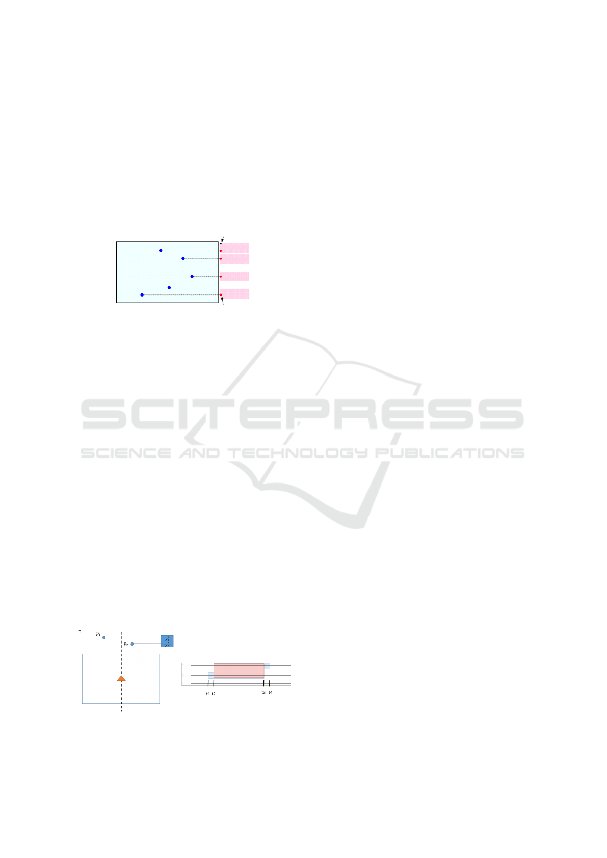
Figure 2: A viewing window with labels placed along the
boundary of the window. Sites are colored in red on the
map.
window is relatively small compared with the size of
the entire map, at any point in time only a portion of
the map along the trajectory can be displayed in the
window. See Fig. 2. In this paper, we consider the
dynamic map labeling problem with sliding labels in
the framework of boundary labeling. A site (or point)
on the map is connected to its associated label at a
port through a horizontal straight-line called a leader.
By sliding labels we mean that a port connecting to
a label can slide on the side of the label. It should
be noted that if two sites are too close to each other,
their labels cannot be displayed simultaneously with-
out causing overlapping. As sites enter and leave the
viewing window in the process of navigating along
the trajectory, our goal is to find a feasible solution
achieving the maximum total visible time of labels
subject to certain requirements. The first requirement
is that labels do not overlap. As pointed out in Been
et al. (Been et al., 2006), label ”jumping” or ”flicker-
ing” should be avoided in dynamic labeling, meaning
that the movement of labels should be continuous in
order not to cause visual disruptions. In our setting,
a trajectory is decomposed into line segments as dis-
played in Fig. 1, in which the route consists of five
segments h
1
, h
2
, h
3
, h
4
and h
5
. The angles between
the five segments are θ
1
, θ
2
, θ
3
, and θ
4
. In our strat-
egy, the optimization procedure is separated into two
modes, namely, moving and rotating modes. When
navigating along a straight line segment (such as those
h
1
, h
2
, h
3
, h
4
and h
5
), a moving mode is involved. At
a junction between, for example h
1
and h
2
, a turn of
θ
1
angle is encountered during which labels may en-
ter and leave the viewing window. Hence, an opti-
mization procedure operating in the rotating mode is
carried out before starting a new phase of a moving
mode.
In the moving mode, we present the objective us-
ing a mixed integer programming (MIP) formulation
with the flickering constraints. By solving the lin-
ear system, non-overlapping label placements with
the maximum total visible time can be found, in spite
of the fact that the running time increases substan-
tially as the input size grows. The rotating mode is a
bit more complicated as it involves non-linear compo-
nents. Our algorithm involves a non-linear program-
ming first, aiming at finding a visible region of an-
gles between each pair of labels, and then apply a lin-
ear programming to carry out the actual label assign-
ments. In order to reduce the running time, we also
propose some heuristic algorithms, capable of find-
ing a feasible solution for most practical applications
in a reasonable amount of time. Experimental results
show our approach to be promising.
The interested reader should note that the main
focus of our work differs from that of (N
¨
ollenburg
et al., 2010) in the sense that (N
¨
ollenburg et al., 2010)
dealt with one-sided boundary labeling subject to con-
tinuously changing the scale of the map as well as
allowing labels to be clustered into smaller groups,
whereas in our setting, our study is w.r.t. a trajectory-
based dynamic boundary labeling. Prior work such
as (Gemsa et al., 2016a; Gemsa et al., 2016b; Gemsa
et al., 2013; Barth et al., 2016) dealt with internal la-
beling in which labels are placed close to the sites to
be labeled inside the map, as opposed to placing la-
bels externally in our setting.
2 PRELIMINARIES
2.1 Boundary Labeling
The boundary map labeling problem can be formu-
lated as follows: given a rectangular viewing window
(or simply view) R and a set of points P, each point
p ∈ P inside the view R is to be assigned (if pos-
sible) to a rectangular label which contains the in-
formation associated with the point. Moreover, each
point should use a straight line or a rectilinear line
(also called a leader) to connect to the associated la-
bel placed on the side of R. Boundary labeling is to
find labels’ positions such that labels do not overlap
with each other, and leaders cannot intersect either.
The point to which a leader is attached is referred to
as a port. A port can be either fixed or sliding. The
former assigns a port to a fixed position of a label (e.g.
the middle of the label), while the latter allows a port
to slide along the side of a label. In general a label can
be placed on one of the four sides of R. An example of
a boundary labeling is depicted in Fig. 3 in which la-
bels are placed on the right side of R. Such a labeling
style is called 1-sided boundary labeling. Throughout
this paper, we consider only 1-sided boundary label-
ing, unless stated otherwise. As labels are placed on
the right side of R, we refer to a label’s upper left-hand
Trajectory-Based Dynamic Boundary Map Labeling
143

corner as the anchor of the label, and a point in R is
connected to a (sliding) port along the left side of the
label through a horizontal straight-line. Notice that
as we use horizontal straight-lines for leaders, at any
point in time there might be points in R that cannot be
labeled without causing overlapping. It is also clear
that for a visible label, the y coordinate of the label’s
anchor (w.r.t. the center of R while the x and y axes
parallel the horizontal and vertical sides of R, respec-
tively) is sufficient to uniquely specify the placement
of the label and well as the port position.
label
label
label
p
1
p
2
p
3
p
4
p
5
label
ancho
r
p
oint
p
ort
leade
r
Figure 3: 1-sided boundary labeling.
2.2 Trajectory-Based 1-Sided Boundary
Labeling
In a typical GIS application, a navigation system com-
putes the optimum route on a map for the user and
renders the output route to guide the user during the
course of the navigation. A way to do so is through
a trajectory map along with a view R which, moving
along the trajectory route, displays the information at
positions of interest to the user (referred to as points)
residing in R using labels. In our study, the label-
ing scheme is based on 1-sided boundary labeling, in
which each point is associated with a label (a rectan-
gle) on the right side of view R. The user’s position
is fixed at the center, and view R and its labels always
align to the user’s view. See Fig. 2. To simplify our
study, we assume the route to consist of a sequence of
line segments as Fig. 1 shows. In our design, we fur-
ther decompose the trajectory into moving and rotat-
ing parts. In the moving part, the user only navigates
the map straight ahead (i.e., in the vertical direction
of R) along the trajectory while in the rotating part,
the user rotates the map’s headway orientation. Fig. 1
illustrates that a trajectory is decomposed into mov-
Figure 4: Timeline and block interval.
ing parts h
1
, . . . , h
5
and rotating part θ
1
, . . . , θ
4
. Using
such a decomposition, we are able to divide the over-
all labeling problem into independent subproblems al-
ternating between moving and rotating. Therefore,
our strategy is to treat the moving and rotating modes
separately, and propose algorithms to solve the prob-
lems individually.
3 LABELING ALGORITHMS
3.1 The Moving Mode
We first consider the case when the view R moves in
the vertical direction upwards. To give the reader a
better feel for how our algorithm works, the idea of
a timeline is used, which is illustrated in Fig. 4. For
more about timelines in dynamic labeling, see also
(Barth et al., 2016). While view R moves upwards in
the vertical direction, points p
2
and p
1
individually
are visible during intervals [t
1
,t
3
] and [t
2
,t
4
], respec-
tively. During [t
2
,t
3
], the two labels, if displayed si-
multaneously, overlap. The time line graph associated
with the two points is shown in Fig. 4(Right). The in-
terval [t
2
,t
3
] is called the block interval between p
1
and p
2
. In the two-point case, the labels of p
1
and p
2
can always be displayed without causing overlapping
as long as their y coordinates are distinct, for a port
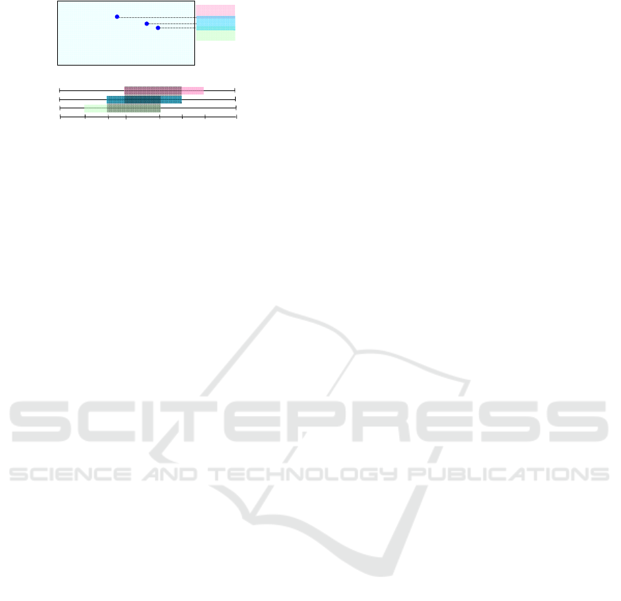
can slide along the left side of a label. Things become
more complicated if an additional point is included
in the view. Fig. 5 shows the timeline together with
the block intervals highlighted in grey for three points
p
1
, p
2
, p
3
. Suppose the y-coordinates of p
1
and p
3
is
smaller than the height of a label (assuming uniform
label height), then between t
3
and t
4
, the three labels
(say, l
1
, l
2
, l
3
) cannot co-exist even under the sliding
port model. In fact, the anchors positions of l
1
, l
2
, l
3
decide the max total visible time of the three labels.
Given a label l, we write (l,t, on) (resp., (l, t, o f f ))
to denote that label l is enabled (resp., disabled) to
display at time t. Consider the following three label
assignments:
• (l
3
,t
1
, on); (l
1
,t
3
, on); (l
3
,t
4
, o f f ); (l
1
,t
6
, o f f ).
In this case, the total visible time is (t
4
−t
1
)+(t
6
−
t
3
).
• (l
3
,t
1
, on); (l
3
,t
2
, o f f ); (l
2
,t
2
, on); (l
2
,t
3
, o f f );
(l
1
,t
3
, on); (l
1
,t
6
, o f f ).
In this case, the total visible time is (t
2
−t
1
)+(t
3
−
t
2
) + (t
6
−t
3
).
• (l
3
,t
1
, on); (l
3
,t
2
, o f f ); (l
2
,t
2
, on); (l
2
,t
3
, o f f );
(l
1
,t
3
, on); (l
1
,t
4
, o f f ); (l
2
,t
4
, on); (l
2
,t
5
, o f f );
(l
1
,t
5
, on); (l
1
,t
5
, o f f ).
IVAPP 2023 - 14th International Conference on Information Visualization Theory and Applications
144

v
l
1
p
3
p
2
p
1
l
3
l
2
t
1
t
2
t
3
t
4
t
5
t
6
Figure 5: Block intervals with three labels.
This is not a legal assignment, as label l
2
is turned
on during [t
2
,t
3
], [t
4
,t
5
] but is off during [t
3
,t
4
],
which results in flickering.
Clearly the first assignment has a higher total visible
time than the second.
We are now in a position to state our problem set-
ting formally in the moving mode.
• (Input:) A map M with a set P = {p
1
, ..., p
n
} of
points, and a trajectory J of a vertical line seg-
ment, a view R with the starting point of the tra-
jectory located at the center of the bottom edge of
R (see Fig. 2).
• (Output:) For each point p
i
∈ P which resides in
the view R at some time during the navigation,
determine the time of interval (possibly empty)
during which p
i
is visible subject to the follow-
ing constraints:
– the label associated with point p
i
is of height
h
i
and is placed on the right size of R through
horizontal (sliding) leaders,
– at any point in time, no two labels can overlap
with each other,
– a label cannot flick, i.e., appear at some time,
disappear later, and reappear at a later time,
– R moves upwards at a constant speed,
such that the total visible time of all labels is max-
imized.
Each point p along the trajectory is associated with
a time interval [t, t
′
] such that p enters and exits R at
t and t
′
, respectively. For ease of expression, we let
P = {p
1
, p
2
, ..., p
n
} be all the points whose time in-
tervals are not empty, i.e., they appear in R at some
point in time along J. We use l
i
to denote the label of
p
i
, and let the time interval of p
i
be [t
i
,t
′
i
], 1 ≤ i ≤ n.
Although R moves along J continuously, it is suffi-
cient to formulate the problem in the discrete case
in which a decision (of whether to display a label
and at which position) is only made at time belong-
ing to T = {t
i
,t
′
i
|1 ≤ i ≤ n}. We sort T and let the
sorted (in increasing order) sequence be r
1
, r
2
, ..., r
m
,
for some m. Let Ψ
j
= [r
j
, r
j+1
], 1 ≤ j ≤ m − 1. We
define |Ψ
j
| = r
j+1
− r
j
, i.e., the length of interval
[r
j
, r
j+1
]. As labels are placed on the right side of
R, it is sufficient to define the position of a label l
i
using the y-coordinate (denoted as y
′
i
) of its anchor
while letting the origin be at the lower left-hand cor-
ner of R at the starting point of J. We let y
i
be the
y-coordinate of p
i
in the same coordinate system. No-
tice that |y
′
i
− y
i
| ≤ h
i
. For each 1 ≤ i ≤ n, we define a
variable x
ik
of value 0 or 1 to indicate whether l
i
is vis-
ible in Ψ
k
or not. Now the problem can be formulated
as the following MIP formulation.
max
n
∑
i=1
m
∑
k=1
x
ik
× |Ψ
k
| ...... (Eq. 1)
subject to
(1) ∀i, j, k, x
ik
+ x
jk
≤ 1 if
min(y
′
i
, y
′
j
) − max(y
′
i
− h
i
, y
′
j
− h
j
) > 0
(2) ∀i, r, s,t, x
ir
+ x
it
≤ x
is
+ 1 if 1 ≤ r < s < t ≤ m
(3) ∀i, k, x
ik
= 0 if Ψ
k
̸⊆ [t
i
,t
′
i
]
In the above MIP, those y
i
,t
i
,t
′
i
, h
i
, 1 ≤ i ≤ n, are
known in advance while variables fall into two
classes:
(i) y
′
i∈R
, 1 ≤ i ≤ n
(ii) x
i j
∈ {0, 1}, 1 ≤ i ≤ n, 1 ≤ j ≤ m.
Notice that the values of y
′
i
decide the timeline as well
as those Ψ
j
. In Eq. 1, (1) is to ensure that overlap-
ping labels are not assigned to the same Ψ
k
; (2) is a
condition to avoid flickering; (3) is obvious as label l
i
associated with point p
i
can only be displayed during
[t
i
,t
′
i
].
In the moving mode, because view R only moves
up along the trajectory, it is desirable to find clusters
of points between which their label assignments can
be done independently. The idea is quite simple. If
the y-distance between two points p
i
and p
j
is larger
than h
i
+ h
j
, their labels have no way of overlapping
regardless where their anchors are located. By search-
ing through the entire set of points along the trajec-
tory, it is easy to identify clusters each of which can
be dealt with separately in the optimization proce-
dure. In our experiment, the above MIP is solved us-
ing the gradient descent approach, and the algorithm
is named Algorithm 1.
To further reduce the running time, a greedy
heuristic can be applied to get rid of type (i) variables
in Eq. 1. The first step is to sort the p
i
, 1 ≤ i ≤ n, ac-
cording to their y-coordinates. For each cluster, we
start by assigning the lower left-hand corner of the la-
bel associated with the top-most point in the sorted
list of the cluster to the y-coordinate of the point, and
the anchor of the label of the lowest point to its y-
coordinate. By doing so, a maximum amount of space
is made available to accommodate the labels of the
Trajectory-Based Dynamic Boundary Map Labeling
145

remaining points. Iteratively, the top-most and the
bottom-most points are chosen from the list whose
anchors have not yet been assigned, and the anchor
of the top-most (resp., bottom-most) point is assigned
in a way to minimize the overlapping with those la-
bels that have been assigned above (resp., below) the
point. The above heuristic algorithm of anchor as-
signment takes O(n) time, even though it may still
result in label overlapping. The next step is to use
the MIP in Eq. 1 to find the best assignment with the
anchor positions of labels given. Such a heuristic al-
gorithm is called Algorithm 2.
3.2 The Rotating Mode
We now consider label assignments in the rotating
mode, in which points may rotate in view R when the
trajectory is turning at a junction between two seg-
ments. While the points are rotating, the existing la-
bels may move up or down which in turn may result
in overlapping. It is also possible to encounter new
points entering the view during the course of the ro-
tation. Like in the moving mode, our objective is to
find the maximum visible time while points are rotat-
ing. Our problem setting in the rotating mode is stated
below.
• (Input:) A map M with a set P of points, a view
R with its center located at c, and an angle of ro-
tation θ
r
.
• (Output:) For each point p ∈ P which resides in
the view R at some time during the course of R
rotating θ
r
degree, determine the time of interval
(possibly empty) during which p is visible subject
to the following constraints:
– the label associated with point p
i
is of height
h
i
and is placed on the right size of R through
horizontal (sliding) leaders,
– at any point in time, no two labels can overlap
with each other,
– a label cannot flick, i.e., appear at some time,
disappear later, and reappear at a later time,
– R rotates θ
r
degree at a constant angular speed
around c,
such that the total visible time of all labels is max-
imized.
In the rotating scenario, the view R rotates at a
constant angular speed w.r.t. the center of R until the
turning angle (i.e., those θ in Fig. 1) is reached. Dur-
ing the rotating mode, points to be labeled could be
either those already in existence (labeled) at the end
of the previous moving mode, or those that enter the
view during the course of the rotation. The mathe-
matical formulation to optimize the total visible time
is more complicated in comparison with the moving
mode, as it involves nonlinear components. As a re-
sult, we apply a two-stage approach to yield solutions
for the problem. We let θ
r
be the angle that the map
turns (assuming that the view is always aligned to the
user’s view) in order to enter the subsequent mov-
ing mode. We assume that all the points involved in
the rotating mode are w.r.t. the coordinate system in
which the origin (0, 0) is at the center of the view R,
and the x and y axes parallel the horizontal and ver-
tical edges of R, respectively, at the point right be-
fore the rotation begins (i.e., at the end of the previous
moving mode). A point p
i
on the map is also recorded
as (r
i
, θ
i
) w.r.t. the polar coordinate system. In order
to keep a leader a straight horizontal line segment, a
label moves up or down (depending on whether the
rotation is counter-clockwise or clockwise) along the
side of the view R. That is, the anchor of a label moves
(w.r.t. the above mentioned coordinate system) in the
process of the rotation.
Consider two points p
i
and p
j
whose labels are
separated initially. Suppose when the map rotates θ
i j
degree clockwise, overlapping begins, and later when
the rotating angle reaches θ
′
i j
the two labels separate
again. In view of the above, θ
′
i j
− θ
i j
can be regarded
as the overlapping region of angle between p
i
and
p
j
, during which the two labels cannot co-exist. The
first stage of our optimization procedure in the rotat-
ing mode is to find out the minimum total pairwise
overlapping regions of angle. More precisely,
min
∑
n
i=1
∑
n
j=1
(θ
′
i j
− θ
i j
) ...... (Eq. 2)
sub ject to
r
i
sin(θ
i
+ θ
i j
) − r
j
sin(θ
j
+ θ
i j
) = h
′
i j
r
i
sin(θ
i
+ θ
′
i j
) − r
j
sin(θ
j
+ θ
′
i j
)
= h
′
i j
− (h
i
+ h
j
)
h
′
i j
= (h
i
− (y
∗
i
− r
i
sin(θ
i
+ θ
i j
))+
(y
∗
j
− r
j
sin(θ
j
+ θ
i j
))
r
i
sin(θ
i
+ θ
i j
) ⩽y
∗
i
⩽ r
i
sin(θ
i
+ θ
i j
) + h
i
r
j
sin(θ
j
+ θ
i j
) ⩽y
∗
j
⩽ r
j
sin(θ
j
+ θ
i j
) + h
j
0 ⩽h
′
i j
⩽ (h
i
+ h
j
)
0 ⩽θ
i j
⩽ θ
r
0 ⩽θ
′
i j
⩽ θ
r
In the above, (r
i
, θ
i
) (resp., (r
j
, θ
j
)) is the polar coor-
dinate of point p
i
(resp., p
j
); y
∗
i
(resp., y
∗
j
), a variable,
is the y-coordinate of the anchor position of p
i
(resp.,
p
j
) w.r.t. the viewing coordinate system (i.e., (0, 0) is
at the center of R, and x and y axes parallel the hor-
izontal and vertical sides of R, resp.); θ
i j
and θ
′
i j
are
IVAPP 2023 - 14th International Conference on Information Visualization Theory and Applications
146

Table 1: Moving mode.
Moving Dataset 1 Dataset 2
Na
¨
ıve Alg. 1 Alg. 2 Na
¨
ıve Alg. 1 Alg. 2
Total Visible Time 0.808 0.870 0.863 0.401 0.526 0.525
Running Time (sec) 0.192 0.373 0.196 3.327 3.493 3.354
Table 2: Rotating mode.
Rotating Dataset 1 Dataset 2
Na
¨
ıve Alg. 3 Alg. 4 Na
¨
ıve Alg. 3 Alg. 4
Total Visible Time 0.58 0.755 0.788 0.495 0.541 0.546
Running Time (sec) 0.938 2141.26 1.513 25.91 39012.84 26.882
also variables. Basically, h
′
i j
is the difference between
the two ports.
As the above objective function considers only
pairwise overlapping region of angle locally, the so-
lution may still result in overlapping labels globally.
The second stage of the optimization is to apply a sim-
ilar approach of using ”timeline” in the moving mode.
Each pair of points p
i
and p
j
have their θ
i j
and θ
′
i j
computed in the previous stage. We mark all the θ
i j
and θ
′
i j
along a timeline, which results in a finite num-
ber of intervals like in the moving mode. Hence, a
formulation like Eq. 1 can be applied to solving the la-
beling problem. Such a two-stage algorithm is called
Algorithm 3.
Even though Eq. 2 provides a good starting point
for constructing the timeline graph, it suffers from a
high time complexity. To ease such a time-consuming
step, a heuristic algorithm similar to the greedy strat-
egy used in Algorithm 2 is also proposed, in which
angles (w.r.t. the coordinate system associated with
the initial view) of all the points involved in the rotat-
ing process are sorted, and a greedy strategy similar
to that in the moving case is applied to assigning an-
chor positions. Incorporating the greedy heuristic in
the rotating mode is called Algorithm 4.
4 EXPERIMENTAL RESULTS
In this section, we present the evaluation of different
algorithms based on the moving and rotating models
which were introduced in Section 3. Our algorithm
was implemented in Python 3.5.2 running on Linux
Ubuntu 16.04. And Gurobi 8 was used for the solver.
Algorithms 1-4 are compared against a simple algo-
rithm in which ports of the labels are at their mid-
dle points. Such a labeling is called the Na
¨
ıve la-
beling in our comparison. Our evaluation takes the
total visible time of labeling and the algorithm’s run-
ning time as the performance metrics. Because we
decomposed the trajectory into moving and rotating
modes, we will show these experiments individually.
Two datasets from OpenStreetMap were used in our
experiments. In our experiments, labels are assumed
to be of uniform height. We first set the label height
to 20, and views R as a 300 × 300 square. So, the
maximum number of the labels that can be displayed
simultaneously is 15. Dataset 1 is a map with less than
25 points, while Dataset 2 contains more than 700
points. The total visible time (in percentage) is mea-
sured against the case when overlapping-free is not
required (i.e., all the labels are displayed even when
they overlap with each others).
4.1 The Moving Case
Fig. 6 shows the labeling results of Dataset 1. No-
tice that the Na
¨
ıve algorithm can only show six labels
in view R (Fig. 6b), while both Algorithm 1 (Fig. 6c)
and Algorithm 2 (Fig. 6d) can show seven labels in
view R. Both Algorithms 1 and 2 slide the highest la-
bel to create space for other labels. However, Table
1 shows that Algorithm 1 can obtain higher total vis-
ible time. The reason is that Algorithm 1 is based on
a precise MIP formulation, whereas Algorithm 2 uses
a greedy heuristic to find appropriate (which may not
be optimal globally) anchors first.
4.2 The Rotating Case
We evaluate the performance, in terms of the total vis-
ible time and the running time, of different algorithms
in the rotating mode. Fig. 7 shows the visual results of
Dataset 1. The number of displayed labels under the
Na
¨
ıve algorithm is less than that using Algorithm 3
and Algorithm 4. There are only six labels in Fig. 7b.
Fig. 7c and 7d show seven labels in view R. The
main difference between Algorithm 3 and Algorithm
4 is the running time. Because Algorithm 3’s ob-
jective function contains trigonometric functions for
each pair of points, it is too complicated to minimize
it. Solving the trigonometric functions is a bottleneck
for the solver, and it is easily beyond the tolerance of
numerical errors. As we can see in Table 2, Algorithm
3 uses much time to solve the minimization problem.
In addition, it could in some cases be stuck at a sad-
dle point of the objective function, causing the total
visible time to be even less than that of Algorithm 4.
The dense point set of Dataset 2 in Table 2 suggests
the same behavior as Dataset 1. As we can see, Al-
gorithms 3 and 4 have a better performance than the
Na
¨
ıve algorithm. However, Algorithm 3 still suffers
from a high running time. As Table 2 shows, using
this heuristic strategy in Algorithm 4 can reduce the
running time substantially.
Trajectory-Based Dynamic Boundary Map Labeling
147

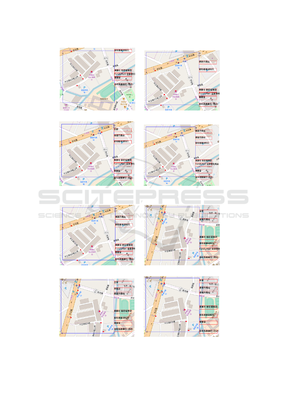
(a) Starting configuration of Dataset 1 (b) Result of the Na
¨
ıve algorithm
(c) Result of Algorithm 1 (d) Result of Algorithm 2
Figure 6: Experimental results of Dataset 1 in the moving mode.
(a) Starting configuration of Dataset 1 (b) Result of the Na
¨
ıve algorithm
(c) Result of Algorithm 3 (d) Result of Algorithm 4
Figure 7: Experimental results of Dataset 1 in the rotating mode.
IVAPP 2023 - 14th International Conference on Information Visualization Theory and Applications
148

4.3 Different Label Heights and
Numbers of Points
We compare the Na
¨
ıve algorithm with Algorithms 1-
4 proposed in this work w.r.t. different label heights.
Tables 3 and 4 show the performance w.r.t. label
height ranging from 10 to 30. Height increasing re-
sults in performance degradation, suggesting that the
number of labels which can be displayed simultane-
ously decreases due to the fact that labels tend to
block more labels. As shown in the tables, Algorithms
1-4 are better than the Na
¨
ıve algorithm in most cases.
Finally, we analyze the running time of Algo-
rithms 1-4. We show Algorithms 1, 2 and 4 on differ-
ent numbers of points ranging from 100 points to 500
points. Table 5 shows their running times. As Algo-
rithm 3 needs to solve the trigonometric functions in
the constraints of the objective function, the problem
size that the algorithm is able to solve in a reasonable
amount of time is rather limited. Table 6 shows the
results of Algorithm 3 for the number of points rang-
ing from 10 to 30. Due to its extremely high running
time, Algorithm 3 is hard to be practical in real-world
applications.
Table 3: Different label heights in the moving mode.
Moving 10 15 20 25 30
Na
¨
ıve 0.626 0.626 0.502 0.439 0.436
Alg. 1 0.839 0.738 0.661 0.502 0.436
Alg. 2 0.837 0.711 0.661 0.502 0.436
Table 4: Different label heights in the rotating mode.
Rotating 10 15 20 25 30
Na
¨
ıve 0.689 0.621 0.542 0.478 0.437
Alg. 3 0.721 0.626 0.558 0.536 0.474
Alg. 4 0.695 0.642 0.558 0.489 0.437
Table 5: Running times of Algorithms 1, 2 and 4 w.r.t. dif-
ferent numbers of points.
100 200 300 400 500
Alg. 1 9.533 32.405 62.303 83.067 152.077
Alg. 2 7.237 29.127 56.037 76.406 127.237
Alg. 4 9.094 37.979 77.51 150.768 237.526
Table 6: Algorithm 3’s running time w.r.t. different num-
bers of points.
10 15 20 25
Running time 1522.768 6079.111 15148.168 30456.744
(sec)
5 CONCLUSIONS
In this paper, we proposed various algorithms for an-
notating trajectory-based dynamic map in the frame-
work of 1-sided boundary labeling. Future research
directions include allowing more sophisticated opera-
tions, such as zooming, scaling, etc, to be performed
during the course of the navigation, as well as relaxing
the number of sides to which labels can be attached.
ACKNOWLEDGEMENTS
The second author was supported in part by National
Science Council, Taiwan, ROC, under Grant MOST
109-2221-E-002-142-MY3.
REFERENCES
Barth, L., Niedermann, B., N
¨
ollenburg, M., and Strash,
D. (2016). Temporal map labeling: a new unified
framework with experiments. In Proc. of 24th Int’l
Conf. on Advances in Geographic Information Sys-
tems, page 23. ACM.
Been, K., Daiches, E., and Yap, C. (2006). Dynamic map
labeling. IEEE Trans. on Visualization and Computer
Graphics, 12(5):773–780.
Bekos, M. A., Kaufmann, M., Symvonis, A., and Wolff,
A. (2007). Boundary labeling: models and efficient
algorithms for rectangular maps. Computational Ge-
ometry, 36(3):215–236.
Fekete, J.-D. and Plaisant, C. (1999). Excentric labeling:
dynamic neighborhood labeling for data visualization.
In Proc. of Conf. on Human Factors in Computing
Systems, pages 512–519. ACM.
Fink, M., Haunert, J.-H., Schulz, A., Spoerhase, J., and
Wolff, A. (2012). Algorithms for labeling focus re-
gions. IEEE Trans. on Visualization and Computer
Graphics, 18(12):2583–2592.
Gemsa, A., Niedermann, B., and N
¨
ollenburg, M. (2013).
Trajectory-based dynamic map labeling. In Proc. of
Int’l Symp. on Algorithms and Computation, pages
413–423. Springer.
Gemsa, A., N
¨
ollenburg, M., and Rutter, I. (2016a). Consis-
tent labeling of rotating maps. Computational Geom-
etry, 7(1):308–331.
Gemsa, A., N
¨
ollenburg, M., and Rutter, I. (2016b). Evalua-
tion of labeling strategies for rotating maps. J. Exper-
imental Algorithmics (JEA), 21:1–4.
Haunert, J.-H. and Hermes, T. (2014). Labeling circular
focus regions based on a tractable case of maximum
weight independent set of rectangles. In Proc. of 2nd
ACM Int’l Workshop on Interacting with Maps, pages
15–21. ACM.
Heinsohn, N., Gerasch, A., and Kaufmann, M. (2014).
Boundary labeling methods for dynamic focus re-
gions. In Proc. of 2014 IEEE Pacific Visualization
Symp. (PacificVis), pages 243–247. IEEE.
N
¨
ollenburg, M., Polishchuk, V., and Sysikaski, M. (2010).
Dynamic one-sided boundary labeling. In Proc. of
18th Int’l Conf. on Advances in Geographic Informa-
tion Systems, pages 310–319. ACM.
Trajectory-Based Dynamic Boundary Map Labeling
149