Interpretability and Explainability of Logistic Regression Model for

Breast Cancer Detection

Emina Tahirovi

and Senka Krivi

Faculty of Engineering and Natural Sciences, International Burch University, Sarajevo 71000, Bosnia and Herzegovina

Faculty of Electrical Engineering, University of Sarajevo, Sarajevo 71000, Bosnia and Herzegovina

Keywords:

Logistic Regression, Explainable AI, Transparency, Healthcare.

Abstract:

Artiﬁcial Intelligence techniques are widely used for medical purposes nowadays. One of the crucial applica-

tions is cancer detection. Due to the sensitivity of such applications, medical workers and patients interacting

with the system must get a reliable, transparent, and explainable output. Therefore, this paper examines the

interpretability and explainability of the Logistic Regression Model (LRM) for breast cancer detection. We

analyze the accuracy and transparency of the LRM model. Additionally, we propose an NLP-based interface

with a model interpretability summary and a contrastive explanation for users. Together with textual explana-

tions, we provide a visual aid for medical practitioners to understand the decision-making process better.

1 INTRODUCTION

An accurate cancer diagnosis is essential for planning

the best action and establishing a treatment plan. Over

a hundred risk factors can simultaneously be involved

in estimating a single post-test probability, making

manual prediction incredibly difﬁcult. Machine learn-

ing models can be beneﬁcial for processing large

numbers of variables and thereby bridging the gap be-

tween risk factors and risk estimation. However, legal

and ethical accountability issues make fully indepen-

dent AI medical systems unlikely. An alternative is

the possibility of developing explainable AI systems,

which would aid humans in decision-making while

keeping the simplicity of its background processes.

Among the numerous computer models used for

predicting clinical outcomes can be distinguished two

main subcategories: models built by the statistics

community and models built by the machine learn-

ing community. Logistic Regression (LR) is a sta-

tistical ﬁtting model widely used to model medical

problems, such as estimating disease risk in coronary

heart disease, breast cancer, prostate cancer, postoper-

ative complications, and stroke. Several studies (Ayer

et al., 2010; Aviv et al., 2009) have shown that LR is a

valuable tool in medical diagnosis since the method-

ology is well established.

As ML models penetrate critical and sensitive

areas such as medicine, what becomes increasingly

challenging is the inability of humans to understand

these models (Lipton, 2018). It is of utter importance

that ML models used in the medical domain can be

trusted. Even if a model achieves high accuracy, it is

still desirable that medical practitioners can decide if

the diagnosis makes sense and that the output is inter-

pretable even to a patient. In a hypothetical scenario,

an LR model would output a cancer diagnosis and ex-

plain why this sample was classiﬁed as a benign or

malignant tumor. The medical practitioner could con-

clude if the patient needs more invasive tests to be

conducted or if the diagnosis is clear enough as is.

A semantic explanation paired with the visualized aid

that clariﬁes the deciding factors and features for a

speciﬁc case can be used for this purpose, which we

propose in this paper.

We propose an Explainable AI (XAI) system for

breast cancer detection consisting of a classiﬁcation

model and semantic and visual models providing the

decision of an LR model together with interpretations

and explanations for a medical practitioner interact-

ing with the system. The classiﬁcation segment is

based on a binary LR model, trained on breast can-

cer characteristics data. The semantic model is an

NLP-based user interface using automated question-

answering models, where the user is prompted to

ask questions about the classiﬁcation of the tumor.

This way, we produce an output tailored to the user’s

needs. We combine the inherent interpretability of LR

with a contrastive explanations approach. Figure 1

gives a diagram explaining this system.

Tahirovi

c, E. and Krivi

c, S.

Interpretability and Explainability of Logistic Regression Model for Breast Cancer Detection.

DOI: 10.5220/0011627600003393

In Proceedings of the 15th International Conference on Agents and Artiﬁcial Intelligence (ICAART 2023) - Volume 3, pages 161-168

ISBN: 978-989-758-623-1; ISSN: 2184-433X

 2023 by SCITEPRESS – Science and Technology Publications, Lda. Under CC license (CC BY-NC-ND 4.0)

161

Figure 1: Diagram of the proposed XAI system for Breast Cancer Detection.

This paper is structured as follows. Section 2 de-

scribes related work. In section 3, we explain LR and

its interpretability and explainability. In section 4, we

start with a brief introduction to the dataset, move on

to explaining our LR model, and ﬁnally present the

NLP semantic user interface. Section 5 presents re-

sults and section 6 concludes the paper.

2 RELATED WORK

The development of machine learning methods made

many breakthroughs in challenging clinical tasks such

as assisted diagnosis, automatic image analysis, and

prediction (Zhao et al., 2020). Logistic Regression

is successfully used for several medical prediction

tasks (Naji et al., 2021; Anisha et al., 2021). The

LR model for binary data is probably the most widely

used in medical research (Hastie et al., 2009). Ayer

et al. (Ayer et al., 2010) compared the performance

of LR and Artiﬁcial Neural Networks (ANNs) on the

Breast Cancer Wisconsin (BCW) dataset, which we

also use in this research. They note that in terms of

clinical interpretation, LR models have better clini-

cal references than ANNs. Sultana and Jilani (Sul-

tana and Jilani, 2018) used Simple Logistic Regres-

sion. They trained the classiﬁer on the BCW dataset.

In their research, this accuracy was higher than any

other classiﬁer, some of which were Nearest Neigh-

bor Classiﬁer, Random Forest, and Decision Tree.

Limitations on the use of deep and ensemble

learning models in the medical domain are reﬂected

in their lack of interpretability (Chakrobartty and El-

Gayar, 2021). Gunning and Aha (Gunning and Aha,

2019) deﬁne XAI as ”AI systems that can explain

their rationale to a human user, characterize their

strengths and weaknesses, and convey an understand-

ing of how they will behave in the future”.

The measures and models involved in decision-

making and solutions to explain them explicitly

had been inspected by Yang et al. (Yang et al.,

2022). They demonstrated the research trends toward

trustable AI and showcased promising XAI results for

the two most widely investigated classiﬁcation and

segmentation problems in medical image analysis.

The fundamental conceptual differences of Ex-

plainable Artiﬁcial Intelligence (XAI) for regression

and classiﬁcation tasks were analyzed by Letzgus et

al. (Letzgus et al., 2021). They focus on ’post-hoc’

explanation where they try to attribute the prediction

for each data sample to its input features in a mean-

ingful manner. They cite contextual utility and feature

importance as the bases of early approaches toward

understanding the decision processes of ML models.

They concluded that explanation methods are favor-

able in the regression scenario and that XAI cannot

be transferred between different types of ML prob-

lems without adaptation.

One point of view that has the potential to broaden

the scope of XAI explanations is contrastive ques-

tions. Cashmore et al. (Cashmore et al., 2019) give

an example of this type of question: ”Why A rather

than B?”. When answering a contrastive explanation,

one must consider a situation where scenario B might

be better suited than scenario A. In other words, one

must consider why scenario B would be more appro-

priate by arguing why scenario A would be less so.

This type of explanation is called a contrastive expla-

nation Krarup et al. (Krarup et al., 2021) argue that

users of explainable user interfaces must be able to

ask explicit contrastive questions.

Natural Language Processing (NLP) may offer a

helping hand in a quest to make medical domain re-

gression tasks more explainable. Krieger (Krieger,

2016) identiﬁes the medical NLP statements used by

medical professionals as gradation words. E.g. ”X-

ray technician A suspects that patient B suffers from

breast cancer”. Modeling such language in an NLP

semantic output could lead to more trust in medical

domain regression tasks. Therefore, we use such lan-

guage to leave an approachable and professional im-

pression.

ICAART 2023 - 15th International Conference on Agents and Artiﬁcial Intelligence

162

3 METHODS

This section describes the proposed approach of an

XAI system consisting of an LR classiﬁer, inter-

pretability, and explainability modules.

3.1 Logistic Regression

Logistic Regression determines the relationship be-

tween a binary outcome (dependent variable) and pre-

dictors (independent variables). It estimates the prob-

ability of an event’s occurrence. It is widely used

in biostatistical applications where binary responses

(two classes) occur quite frequently (Hastie et al.,

2009). In the medical problem, we address the two

classes which make the binary response 1 for malig-

nant tumors and 0 for benign. Here, the diagnosis is

the dependent variable, and the parameters which de-

scribe the cancer cells are the independent variables.

Let y denote the presence of the disease, where

y = 0 or y = 1, and let x denote the vector of predic-

tors (features). Given that p denotes the probability

of breast cancer (the probability that y = 1), we can

deﬁne Logistic Regression with

P(y = 0, 1|x, w) =

1 + e

−(w

x+b)

(1)

Here, (w, b) are weights, with b being a constant,

w the regression coefﬁcients to their respective pre-

dictor variables x, and y the class label. These coefﬁ-

cients are estimated from the available data.

If the training instances are from the dataset

M = (x

, y

), ..., (x

, y

) with the labels y

∈ {0, 1},

one estimates (w, b) by minimizing the negative log-

likelihood: min

w,b

∑

i=1

log(1 + e

−(w

+b)

) (2).

3.2 Interpretability of Logistic

Regression

An oft-made claim is that linear models are preferable

to deep neural networks because of their interpretabil-

ity. The high accuracy of complex models comes at

the expense of interpretability. Hence, even the con-

tributions of individual features to the predictions of

such a model become challenging to understand (Lou

et al., 2012). Interpretability can be seen as a reﬂec-

tion of several different ideas than a monolithic con-

cept (Lipton, 2018). Another view of interpretability

is that it represents the degree to which a human can

understand the cause of a decision (Miller, 2019).

While the output of the LR model is binary, the

precedent of this output is a probability output in the

range from 0 to 1. The probability output is trans-

formed into the binary output by using a cutoff value

of 0.5. A positive classiﬁcation (= 1) is the result

of a probability of ≥ 0.5, and a negative classiﬁca-

tion (= 0) is the result of a probability of < 0.5. We

use this probability of each classiﬁcation as an inter-

pretability approach, essentially utilizing an aspect of

LR’s inherent interpretability. By analyzing Eq.(1) we

get

P(y = 1|x, w)

1 − P(y = 1|x, w)

P(y = 1|x, w)

P(y = 0|x, w)

= e

x+b

(2)

We can now examine how the feature weights and

values affect the probability. Let us say that x is a

vector of x

, ..., x

∈ N variables, and feature values of

changes from x

= a to x

= c where c−a = 1. Now

we can examine how the change of the feature from a

to c impacted the model’s outcome by observing the

ratio the probability gets scaled by a factor of e

we can deduce from:

(b+w

+...+cw

+...+w

)

(b+w

+...+aw

+...+w

)

= ... = e

(a+1)w

−aw

= e

(3)

To highlight this impact for a user and provide the

interpretability of the decision, we use the following

plots:

1. Sigmoid plot, to clarify to the user where the cur-

rently observed cancer sample lies on the plot,

2. value counts plots to clarify the dominance of fea-

ture values for each classiﬁcation, and

3. classiﬁcation shift at the classiﬁcation border with

changing values of x

3.3 Explainability of Logistic

Regression

If we look at LR as a classiﬁcation model, there is im-

plicit knowledge associated with the class. This can

serve as a piece of a potential explanation of LR (Let-

zgus et al., 2021). The explainability of a model de-

pends on the level of known information about how

the parameters of a model impact the decision pro-

cess. In this respect, the coefﬁcients of an LR model

make it directly explainable. Hence, as valuable infor-

mation for the user, we select visualization of feature

importance.

Another important aspect that needs to be kept in

mind when developing XAI models is the recipient

of the information. The information must be tailored

to the end user. As our interface is meant to be used

by medical personnel, we tailor our explanations in a

way that will help relate their pre-existing knowledge

on the topic, while helping them understand how our

model makes predictions. The explainability of our

model relies on three different methods:

Interpretability and Explainability of Logistic Regression Model for Breast Cancer Detection

163

• identiﬁcation of a relevant subset of features,

• interpretation of feature importance scores,

• explainability by contrastive example.

We present feature importance plots, parallel

plots, classiﬁcation shift plots, box plots, and heat

maps to help the end user understand what kind of

data leads to a certain prediction.

Contrastive Explanation: is a speciﬁc type of

explanation which answers a question of type: ”Why

A rather than B ?”. It includes a contrastive exam-

ple with the goal of presenting the difference in the

decision-making to the user. It is commonly used in

various AI ﬁelds (Krarup et al., 2021). In our medical

XAI system case, we propose presenting two different

feature vectors x

and x

c f

as contrastive examples of

feature vectors to the user. For the current input vec-

tor x

and the decision of an LR classiﬁer y

, we deﬁne

these contrastive vectors as follows. x

is the value

of a feature vector with minimal Euclidean distance

from the input vector x

which results in the opposite

class result ¬y

. x

c f

is a vector in which variation in

a single feature value results in the prediction class

change and becomes ¬y

4 IMPLEMENTATION DETAILS

XAI MEDICAL SYSTEM

This section explains the dataset used for this research

and the implementation process. In the ﬁrst subsec-

tion, we go through the nature of the dataset and its

features. In the following subsections, we explain the

implementation of the LR model and the NLP seman-

tic user interface.

4.1 Dataset Description

The dataset used for this research is the well-known

Wisconsin Breast Cancer Dataset obtained from the

UC Irvine Machine Learning Repository (Mangasar-

ian et al., 1995). The nine predictor variables ana-

lyzed for this research are visually assessed cytologi-

cal characteristics of a Fine Needle Aspiration (FNA)

sample. These variables take integer values between

1 and 10. Wolberg and Mangasarian (Wolberg and

Mangasarian, 1990) chose the nine features based on

statistical analysis, which showed a signiﬁcant dif-

ference in values for benign and malignant samples.

Therefore, they are prominent candidates for predic-

tor variables for our LR model. These predictor vari-

ables are uniformity of cell shape, uniformity of cell

size, clump thickness, marginal adhesion, single ep-

ithelial cell, bare nuclei, bland chromatin, normal nu-

cleoli, and mitosis. The feature class is the predicted

or the dependent variable in this dataset.

4.2 Logistic Regression Model

Our LR model is implemented from scratch, in

Python, on the Jupyter Notebook platform. It is a bi-

nary LR model with an added bias term. The moti-

vation behind the from-scratch implementation is the

interpretability of each step of LR, where one can

choose to print out different values and interpret them

separately, as opposed to a black-box approach to LR

with a library-provided model.

The original model is trained on all 9 features and

is evaluated using stratiﬁed 5-fold cross-validation.

These preliminary scores are 97.10% for accuracy,

and 95.65% for F

-score. Models trained on differ-

ent subsets of features are cross-validated individu-

ally. Each subset consists of n most important fea-

tures, as determined by feature importance scores (see

subsection 5.2). The results are recorded and the best-

performing model is selected. The optimal subset size

was determined to be 7 features, which are, in order

of importance: bare nuclei, clump thickness, mitosis,

uniformity of cell shape, marginal adhesion, bland

chromatin, and normal nucleoli. This model is our

ﬁnished LR model.

4.3 NLP Models and User Interface

The output of our framework is based on an NLP ex-

plainable user interface, which produces a combina-

tion of textual and pictorial explanations to provide

aid for medical practitioners to better understand the

decision-making process of the LRM. In the follow-

ing subsections, we explain the models used to imple-

ment this user interface.

Word2Vec: is a word embedding model. It is an

unsupervised learning algorithm that generates low-

dimensional vector representations of words. The

variation used in this research is Skip-gram, which

predicts the context, given the word.

GloVe: or global vectors is an unsupervised learn-

ing algorithm that obtains low-dimensional vector

representations for words and performs dimensional-

ity reduction on the word context matrix. It thereby

keeps track of the frequencies of word co-occurrences

in a text, with an additional weight parameter depen-

dent on the distance between the words.

Question Database: consists of twenty-two ques-

tions and their respective answers. Some of these an-

swers are static, while others are assembled with the

help of the information obtained from the model. The

database is shown in table 1. Answers to questions

ICAART 2023 - 15th International Conference on Agents and Artiﬁcial Intelligence

164

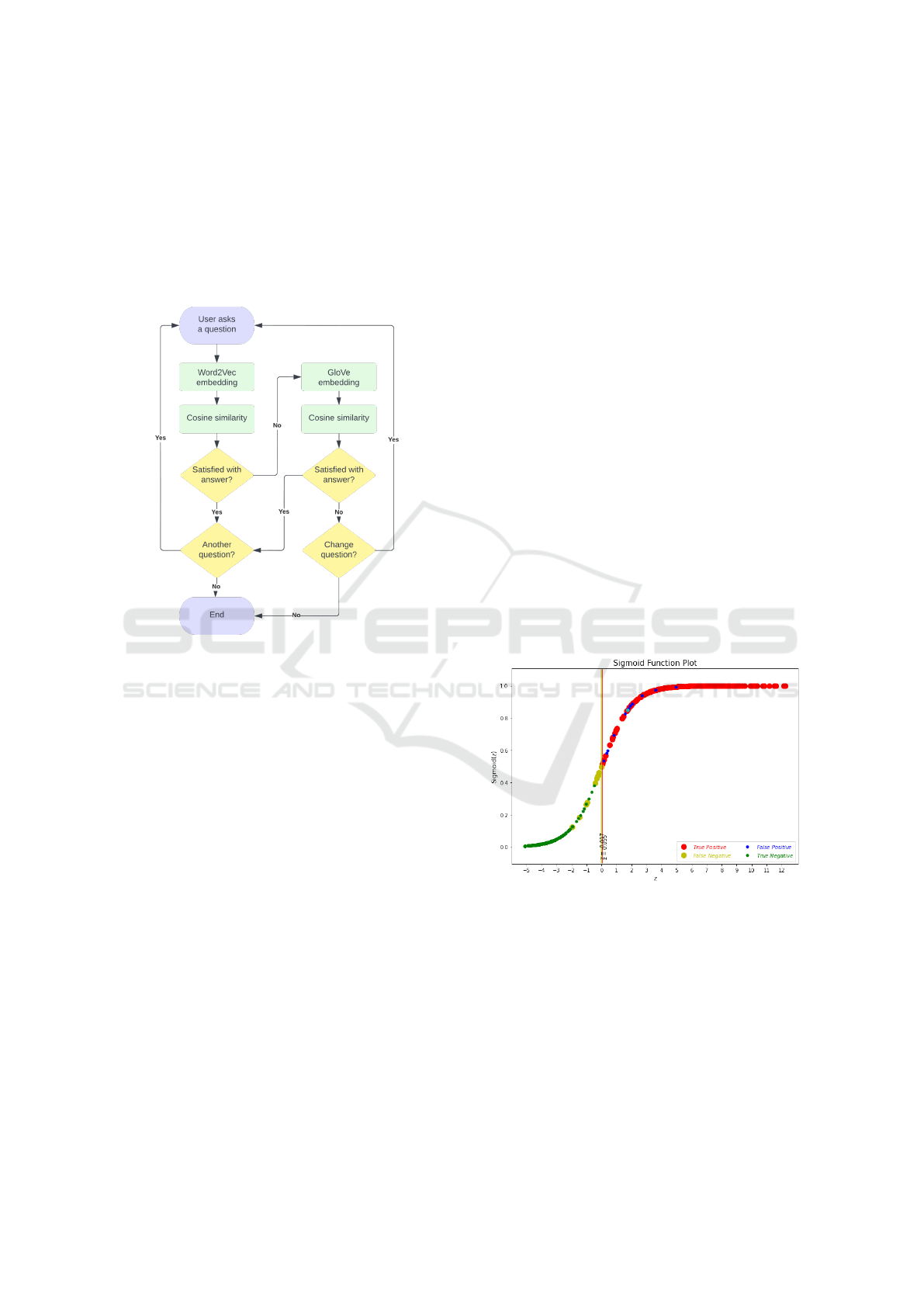
13-22 are explained in section 5.2.

Automated Question Answering: The next level

of interpretability is reached through an NLP auto-

mated question-answering model based on Word2Vec

or GloVe embeddings. We use cosine similarity to es-

timate how similar the user-asked question is to the

questions in the database. The process is illustrated

from start to ﬁnish in ﬁgure 2.

Figure 2: User interface state diagram.

5 EXPERIMENTAL RESULTS

This section presents the prediction, interpretability,

and explainability results of our models. We provide

textual, as well as pictorial explanations of our results.

5.1 LR Prediction Evaluation

We present the prediction results of our model in

Table 2 for the test subset and the original dataset.

For the performance evaluation, we compare the CV

score, accuracy, precision, recall, and F1 score. Ta-

ble 3 shows the confusion matrices for the test set

and complete dataset. These results indicate that our

model performs well, as the rates of falsely classiﬁed

data are low. The ratio of each portion (true positives,

false positives, false negatives, and true negatives) is

well-preserved in the test set, as evident from compar-

ing the test and entire dataset confusion matrices.

5.2 Interpretability Results

When the user begins the interaction with our inter-

face, they are presented with some basic information

about how their tumor is seen by our model. They are

told what their classiﬁcation is (benign or malignant),

and how probable it is that the tumor is malignant.

Figure 3 shows the Sigmoid plot for the entire

dataset, where the colors of the dots are clariﬁed by

the legend. The two vertical bars represent the right-

most negative and the left-most positive classiﬁcation,

along with their respective Z-values. The currently

observed cancer sample is represented by a cyan dot.

This ﬁgure is presented along with the answer to

question no. 13 in the semantic output (see Table 1).

Its purpose is to clarify to the user where the currently

observed cancer sample lies on the plot and to get a vi-

sual sense of how similar this sample is to other such

classiﬁcations.

In this way, we maintain a level of transparency

as to how our model classiﬁes data. This plot is

presented in combination with a textual output stat-

ing the density of falsely classiﬁed samples in the

0.5-neighborhood of the current cancer sample (along

the Z-axis), the values of each of the 7 relevant fea-

tures, and the space between the left-most positive

and right-most negative classiﬁcation. These state-

ments aim to help the user interpret the classiﬁcation.

Figure 3: Sigmoid plot for the entire dataset.

Figure 4 shows the percentages of value counts for

bare nuclei, for benign and malignant samples. Anal-

ogous plots are generated for all other features. These

plots are used in questions 14 and 15 to clarify the dif-

ferences in the values that the individual features typ-

ically take for different classiﬁcations. This way, the

user can clearly see that for example bare nuclei=1 is

most often seen in benign samples.

Figure 5 shows the shift of the classiﬁcation prob-

ability of the observed tumor sample with the change

of a single feature, in this case, bare nuclei. This plot

Interpretability and Explainability of Logistic Regression Model for Breast Cancer Detection

165

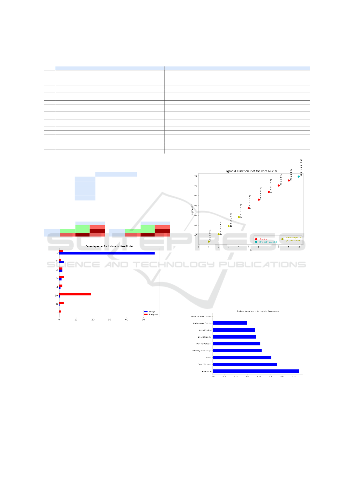
Table 1: Questions database.

Questions Answers

1 Why is the tumor classiﬁed as malignant?

The parameters of this tumor produced a similar function value to the tumors

which have previously been marked malignant by a human doctor. Your parameters are:

2 Why is the tumor classiﬁed as benign?

The parameters of this tumor produced a similar function value to the tumors

which have previously been marked benign by a human doctor. Your parameters are:

3 What does ’malignant’ mean? Malignant tumors are cancerous (i.e., they invade other sites).

4 What does ’benign’ mean? Benign tumors are those that stay in their primary location without invading other sites of the body.

5 How similar is this tumor to tumors which have been classiﬁed as False Positive?

Your tumor falls in the range of tumors that are known to have been correctly classiﬁed

as negative, i.e. were True Positive and had no similar False Positive points nearby.

6 How similar is this tumor to tumors which have been classiﬁed as False Negative? Your tumor is not classiﬁed as benign, therefore it is not similar to other such data points.

7 Should I get additional tests done?

Additional tests are not considered necessary in cases similar to yours.

However, consult your specialist about the best course of action.

8 What do ’benign’ and ’malignant’ mean?

Benign tumors are those that stay in their primary location without invading other sites of the body.

Malignant tumors are cancerous (i.e., they invade other sites).

9 What is the difference between ’benign’ and ’malignant’?

Benign tumors are those that stay in their primary location without invading other sites of the body.

Malignant tumors are cancerous (i.e., they invade other sites).

10 What is the next course of action? The next course of action for your tumor should be consulted with your specialist.

11 What are some similar samples and their likelihoods? Point X was found to be in the 5 most similar points to your sample. It has a Y probability of being malignant.

12 What is the treatment plan for my tumor? The treatment plan should be consulted with your specialist.

13 Can I see my tumor’s data point visualized? Here is your tumor data visualized:

14 Which feature values prevail for malignant tumors? Here you can see approximate percentages of either classiﬁcation per feature per value:

15 Which feature values prevail for benign tumors? Here you can see approximate percentages of either classiﬁcation per feature per value:

16-22 How does the classiﬁcation shift with changing the value of feature X? This is how your tumor classiﬁcation changes with changing the value of feature X:

Table 2: Evaluation of LR model.

Test set Whole set

CV score / 100.00%

Accuracy 98.55% 96.93%

Precision 95.83% 95.42%

Recall 100.00% 95.82%

F1-score 97.87% 95.62%

Table 3: Confusion matrix for the test set (left) and the

whole dataset (right) for LR model trained on 7 features.

Actual Actual

Positive Negative Positive Negative

Positive 45 1 Positive 433 11

Predicted

Negative 0 23

Predicted

Negative 10 229

Figure 4: Class percentages plot for bare nuclei.

is shown along with the answer to questions no. 16-22

(one question per feature), for the purposes of visually

clarifying the impact of the individual features on the

classiﬁcation shift of the currently observed cancer

sample. In this way, we clearly show how changing

the value of just one feature impacts the classiﬁcation.

5.3 Explainability Results

Figure 6 shows the feature importance scores for our

LR model, which are also the model weights. These

scores explain which features had the most impact on

the prediction. It can be noticed from the plot that

Figure 5: Changing the value of bare nuclei for the observed

tumor sample.

the feature bare nuclei contributes most to the clas-

siﬁcation outcome, which means that it will have the

greatest ”pull” in deciding how the tumor is classiﬁed.

This plot clearly shows how important each feature is

for the prediction outcome.

Figure 6: Feature importance scores for the LR model.

Figure 7 shows the heat maps for the malignant

and benign portions of the data. Upon visual inspec-

tion, it becomes obvious that these two portions differ.

For example, features marginal adhesion and bland

chromatin have a correlation of 0.33 for the posi-

ICAART 2023 - 15th International Conference on Agents and Artiﬁcial Intelligence

166

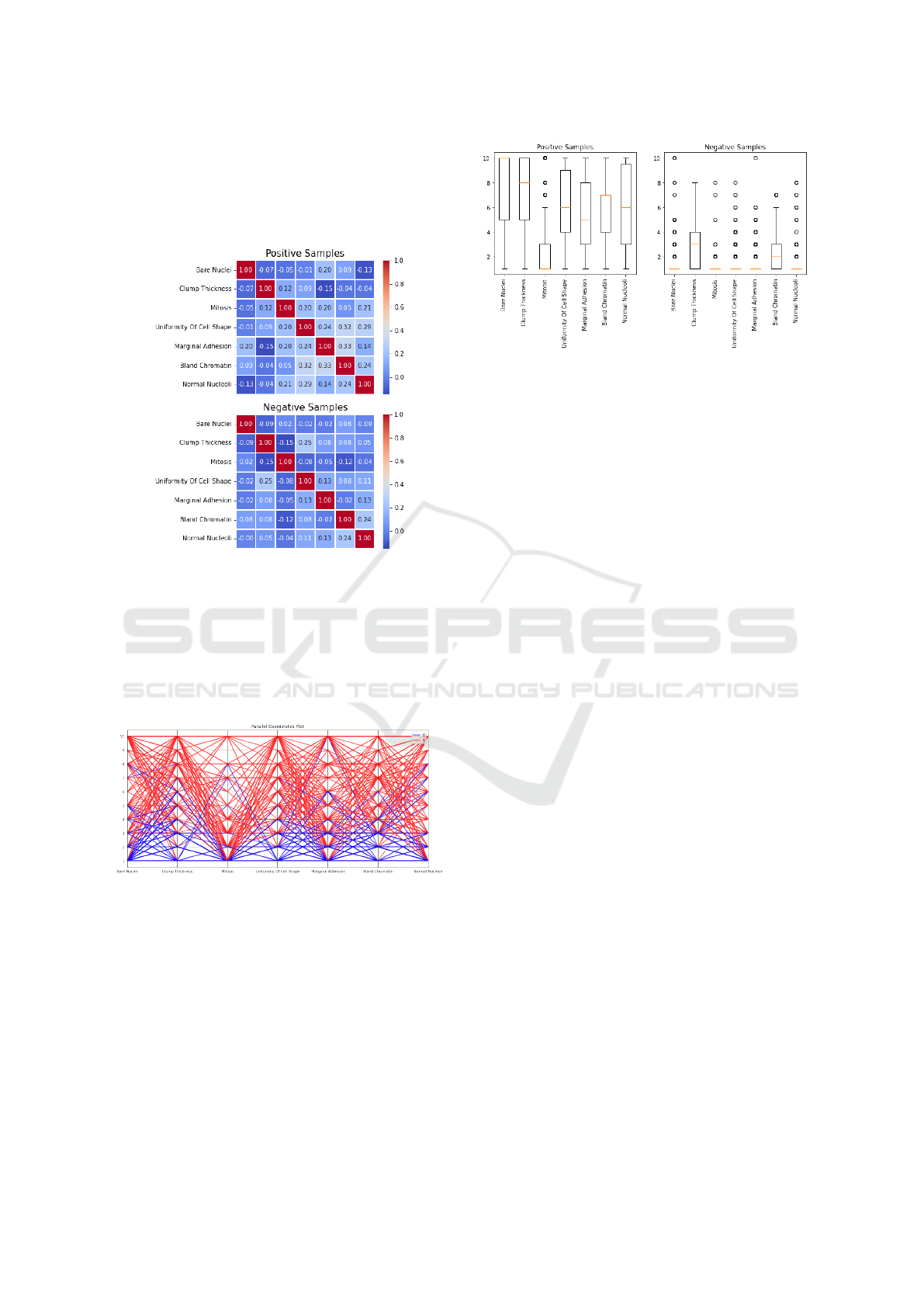
tive portion, and -0.02 for the negative portion of the

dataset. Many more similar examples can be found in

the heat maps. This plot shows how features manifest

different relationships between malignant and benign

tumors.

Figure 7: Heat maps for the LR model for positive (malig-

nant) and negative (benign) portions of the data.

Figure 8 shows the parallel coordinates plot for the

malignant and benign portions of the data. One can

infer simply by looking at this graph that the features

tend to take lower values for the benign portion of

the dataset, while the malignant portion tends to take

higher values. This can also be inferred from ﬁgure 4.

Figure 8: Parallel coordinates plot for positive (1=malig-

nant) and negative (0=benign) portions of the dataset.

Figure 9 shows the box plots for positively and

negatively classiﬁed samples. Again, it is clear that

the positive and negative samples behave differently.

For instance, the median values and ranges are dif-

ferent for all features. Feature values for 5 out of 7

features in the negative portion are scattered across

the plot. These plots conﬁrm that the malignant and

benign portions of the data have different statistical

properties.

To better explain the effect that the values of the

features have on the classiﬁcation of the tumor, we

Figure 9: Box plots for the whole dataset.

ﬁnd the space of possible solutions for Sigmoid(Z) −

0.5 < ε, ε = 1 × 10

−6

. This way, we show how mov-

ing the values along their respective ranges affects the

shift in classiﬁcation at the classiﬁcation border.

Figure 10 shows the classiﬁcation shift at the clas-

siﬁcation border while moving the values of the fea-

ture bare nuclei along its range. Analogous ﬁgures

are generated for all other features. These ﬁgures help

explain how changing even a single feature’s value af-

fects the classiﬁcation.

If we try to imagine the vector of 7 features as a

vector in 7-dimensional Euclidean space, where each

feature represents a single dimension, then we can

also imagine that the illustrated changes are step-wise

changes per dimension. This way, especially illus-

trative are the ﬁgures where the classiﬁcation had

changed, but the step-wise shift per dimension is only

one step away from the original vector. This can,

for example, be observed for feature bare nuclei,

where changing the value of bare nuclei from 3 to

2, while the values of the other features remain con-

stant, changes the output of Sigmoid(Z) from close to

0.5 but positive, to signiﬁcantly less than 0.5.

Another interesting connection can be made be-

tween the weights of the features and the classiﬁca-

tion shifts plot. Namely, it can be observed that the

Sigmoid(Z) values always increase as X

increases,

where i is the currently observed feature. This is be-

cause the weights of the features are all positive.

6 CONCLUSION

In this paper, we presented a framework for breast

cancer prediction and output interpretation based on

Logistic Regression and NLP methods. The inherent

interpretability of Logistic Regression was used as the

foundation of the quest toward interpretability, while

the pursuit of explainability focused on explaining the

preferred data of each class. While Logistic Regres-

sion is commonly used in clinical and health services

Interpretability and Explainability of Logistic Regression Model for Breast Cancer Detection

167

Figure 10: Classiﬁcation shift at classiﬁcation border for

bare nuclei.

as a powerful tool, it is important not to forget its lim-

itations, such as the assumption of the absence of high

intercorrelations among the predictors. Therefore, in

future work, we will examine the XAI setup for med-

ical applications with more powerful methods such as

Deep Learning.

Our contribution is a completely transparent, in-

terpretable, and explainable model, developed with

the purpose of aiding medical personnel in the

decision-making process. It contributes towards ex-

tending XAI to regression models, by adapting an

NLP method as a way to access desired explanations.

In future work, we plan to perform user experiments

in order to rate the helpfulness of our model.

REFERENCES

Anisha, P., Reddy C, K., Apoorva, K., and Mangipudi, C.

(2021). Early diagnosis of breast cancer prediction

using random forest classiﬁer. IOP Conference Series:

Materials Science and Engineering, 1116:012187.

Aviv, R. I., d’Esterre, C. D., Murphy, B. D., Hopyan, J. J.,

Buck, B., Mallia, G., Li, V., Zhang, L., Symons, S. P.,

and Lee, T.-Y. (2009). Hemorrhagic transformation of

ischemic stroke: Prediction with ct perfusion. Radiol-

ogy, 250(3):867–877.

Ayer, T., Chhatwal, J., Alagoz, O., Kahn, C. E., Woods,

R. W., and Burnside, E. S. (2010). Comparison of

logistic regression and artiﬁcial neural network mod-

els in breast cancer risk estimation. RadioGraphics,

30(1):13–22.

Cashmore, M., Collins, A., Krarup, B., Krivic, S., Maga-

zzeni, D., and Smith, D. E. (2019). Towards explain-

able AI planning as a service. CoRR, abs/1908.05059.

Chakrobartty, S. and El-Gayar, O. F. (2021). Explainable

artiﬁcial intelligence in the medical domain: A sys-

tematic review. In Chan, Y. E., Boudreau, M., Aubert,

B., Par

e, G., and Chin, W., editors, 27th Americas

Conference on Information Systems. Association for

Information Systems.

Gunning, D. and Aha, D. W. (2019). Darpa’s explain-

able artiﬁcial intelligence (XAI) program. AI Mag.,

40(2):44–58.

Hastie, T., Tibshirani, R., and Friedman, J. H. (2009). The

Elements of Statistical Learning: Data Mining, Infer-

ence, and Prediction, 2nd Edition. Springer Series in

Statistics. Springer.

Krarup, B., Krivic, S., Magazzeni, D., Long, D., Cashmore,

M., and Smith, D. E. (2021). Contrastive explanations

of plans through model restrictions. J. Artif. Intell.

Res., 72:533–612.

Krieger, H. (2016). Capturing graded knowledge and uncer-

tainty in a modalized fragment of OWL. In van den

Herik, H. J. and Filipe, J., editors, Proceedings of the

8th International Conference on Agents and Artiﬁcial

Intelligence, Vol.2, pages 19–30. SciTePress.

Letzgus, S., Wagner, P., Lederer, J., Samek, W., M

uller, K.,

and Montavon, G. (2021). Toward explainable AI for

regression models. CoRR, abs/2112.11407.

Lipton, Z. C. (2018). The mythos of model interpretability.

Commun. ACM, 61(10):36–43.

Lou, Y., Caruana, R., and Gehrke, J. (2012). Intelligible

models for classiﬁcation and regression. In The 18th

ACM SIGKDD International Conference on Knowl-

edge Discovery and Data Mining, KDD ’12, 2012,

pages 150–158. ACM.

Mangasarian, O. L., Street, W. N., and Wolberg, W. H.

(1995). Breast cancer diagnosis and prognosis via lin-

ear programming. Oper. Res., 43(4):570–577.

Miller, T. (2019). Explanation in artiﬁcial intelligence: In-

sights from the social sciences. Artif. Intell., 267:1–

38.

Naji, M. A., Filali, S. E., Aarika, K., Benlahmar, E. H., Ab-

delouhahid, R. A., and Debauche, O. (2021). Machine

learning algorithms for breast cancer prediction and

diagnosis. Procedia Computer Science, 191:487–492.

Sultana, J. and Jilani, A. K. (2018). Predicting breast cancer

using logistic regression and multi-class classiﬁers.

International Journal of Engineering & Technology,

7(4.20).

Wolberg, W. H. and Mangasarian, O. L. (1990). Multisur-

face method of pattern separation for medical diag-

nosis applied to breast cytology. Proceedings of the

National Academy of Sciences, 87(23):9193–9196.

Yang, G., Ye, Q., and Xia, J. (2022). Unbox the black-box

for the medical explainable ai via multi-modal and

multi-centre data fusion: A mini-review, two show-

cases and beyond. Information Fusion, 77:29–52.

Zhao, Y., Yang, F., Fang, Y., Liu, H., Zhou, N., Zhang,

J., Sun, J., Yang, S., Menze, B. H., Fan, X., and

Yao, J. (2020). Predicting lymph node metastasis

using histopathological images based on multiple in-

stance learning with deep graph convolution. In 2020

IEEE/CVF Conference on Computer Vision and Pat-

tern Recognition, CVPR 2020, Seattle, WA, USA,

June 13-19, 2020, pages 4836–4845. Computer Vision

Foundation / IEEE.

ICAART 2023 - 15th International Conference on Agents and Artiﬁcial Intelligence

168