Point Cloud Neighborhood Estimation Method Using Deep

Neuro-Evolution

Ahmed Abouelazm, Igor Vozniak, Nils Lipp, Pavel Astreika and Christian Mueller

Deutsches Forschungszentrum f

ur K

unstliche Intelligenz (DFKI), Saarbruecken, Germany

Keywords:

Point Clouds, 3D Deep Learning, Neighborhood Estimation, Deep Neuro-Evolution.

Abstract:

Due to the recent advancements in computing hardware, deep learning, and 3D sensors, point clouds have

become an essential 3D data structure, and their processing and analysis have received considerable attention.

Given the unstructured and irregular nature of point clouds, encoding local geometries is a signiﬁcant barrier in

point cloud analysis. The aforementioned challenge is known as neighborhood estimation, and it is commonly

addressed by ﬁtting a plane to points within a local neighborhood deﬁned by estimated parameters. The

estimated neighborhood parameters for each point should adapt to the point cloud’s irregularities and different

local geometries’ sizes and shapes. Different objective functions have been derived in the literature for optimal

parameters selection with no efﬁcient approach for these objective functions’ optimization as of now. In this

work, we propose a novel neighborhood estimation pipeline for such optimization which is objective function

and neighborhood type invariant, utilizing a modiﬁed version of deep Neuro-Evolution algorithm and Farthest

Point Sampling as an intelligent sampling approach. Results demonstrate the ability of the proposed pipeline

for state-of-the-art objective functions optimization and enhancement of neighborhood properties estimation

such as the normal vector.

1 INTRODUCTION

RGB images have long been the focus of image pro-

cessing and computer vision research. Furthermore,

the fast development of deep learning has aided the

rise of 2D images as a dominant data structure (Chai

et al., 2021). However, we live in a three-dimensional

world, and the capacity of two-dimensional images to

fully depict three-dimensional objects in the world is

limited. This is due to the fact that RGB images do not

capture depth information and instead project data on

a single depth 2D plane. Furthermore, RGB images

are sensitive to illumination and lack contrast. Due

to the importance of depth information in understand-

ing the geometry of a scene, algorithmic techniques

for depth estimation from single and stereo images

have been investigated in the literature (Ming et al.,

2021; Lazaros et al., 2008). Despite the success of

these techniques, 3D sensors that can directly capture

depth without estimation are required. Thus, several

3D data formats have been proposed in recent years,

such as point clouds and RGB-D images. Due to the

rapid development of 3D acquisition devices such as

LiDAR and RGB-D sensors, as well as the decrease

in their cost, 3D data structures have been expanded

to a variety of applications nowadays such as robotics

and autonomous driving (Royo and Ballesta-Garcia,

2019). One of the most prevalent 3D data structures

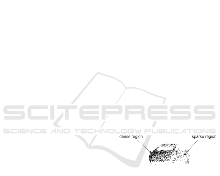
Figure 1: Challenge of neighborhood estimation on an ir-

regular point cloud (Bello et al., 2020), as the point cloud

has sparse and dense regions, which requires adapting

neighborhood parameters.

is Point Cloud Data (PCD), which is a representation

generated by LiDAR sensors. PCD is a 3D format

that depicts a scanned object as a set of discrete points

scattered in a Euclidean space. Each point representa-

tion can be augmented by color, normal vector at the

point of interest, and other feature descriptors. De-

spite becoming increasingly popular in the research

community, PCDs still face the following main dis-

advantages which must be considered during analysis

and processing. PCD is an unordered set of points that

lacks any underlying structure or regular grid. Be-

sides, it is an irregular data type with some regions

having high density, large number of points per unit

582

Abouelazm, A., Vozniak, I., Lipp, N., Astreika, P. and Mueller, C.

Point Cloud Neighborhood Estimation Method Using Deep Neuro-Evolution.

DOI: 10.5220/0011627300003417

In Proceedings of the 18th International Joint Conference on Computer Vision, Imaging and Computer Graphics Theory and Applications (VISIGRAPP 2023) - Volume 4: VISAPP, pages

582-593

ISBN: 978-989-758-634-7; ISSN: 2184-4321

 2023 by SCITEPRESS – Science and Technology Publications, Lda. Under CC license (CC BY-NC-ND 4.0)

volume, whereas others are sparse, with just a few

points as depicted on ﬁgure 1.

The challenges as mentioned earlier require per-

mutation invariant density aware methods for encod-

ing local geometries and local correlations between

points in a PCD. Local geometries are commonly en-

coded by extracting features from a plane ﬁtted to a

neighborhood, where the points included in the neigh-

borhood are determined by a set of parameters, for

each point in the PCD. The estimation of these pa-

rameters is known as neighborhood estimation (Wein-

mann et al., 2015; Demantk

e et al., 2011), and it

is a critical step for the majority of machine learn-

ing techniques used in PCD processing. Since the

attributes initially retrieved using neighborhood es-

timation can be used for more complex tasks such

as keypoints detection and feature descriptors (Ciru-

jeda et al., 2014; Huang and You, 2012; Siritanawan

et al., 2017; Zhong, 2009). Furthermore, neighbor-

hood estimation is not only essential for machine

learning techniques but has also been integrated into

deep learning modules (Liu et al., 2019; Suo et al.,

2020; Zhao et al., 2022; Yang et al., 2018).

Due to the obvious irregular nature of PCDs, as

illustrated on ﬁgure 1, ﬁtting a neighborhood with the

same parameters throughout the PCD is inappropriate

as these parameters should vary between dense and

sparse regions and take into account the dimensional-

ity and size of local geometries present in the PCD.

In the literature, several neighborhood types and two

objective functions have been proposed for optimal

neighborhood estimation (Weinmann et al., 2015; De-

mantk

e et al., 2011). However, to the best of our

knowledge, no effective pipeline exists to optimize

these suggested objective functions, except for a grid-

based search with ﬁxed resolution presented in (De-

mantk

e et al., 2011; Weinmann et al., 2015). The pro-

posed grid search requires exhaustive iteration over a

discrete set of neighborhood parameters ﬁxed for all

points, and doesn’t have the ability to generalize to

similar points.

The contribution of this work is the design

and validation of a novel and computationally efﬁ-

cient (requires fewer training parameters; no back-

propagation step is involved, thus, less used mem-

ory) pipeline for explicit and optimal neighborhood

estimation using a learning module in an unsuper-

vised manner. The learning module learns optimal

parameter selection from a small subset of points and

generalizes the learned selection across the remain-

ing points in the PCD, thus enhancing computation

and memory efﬁciency while ﬁnding an accurate solu-

tion. An effective subset of points for learning is sam-

pled using Farthest Point Sampling (FPS) (Eldar et al.,

1994) as it has the ability to sample points that provide

sufﬁcient information about the point cloud structure.

The novelty of this work is twofold: a) we propose

to use a modiﬁed version of Deep Neuro-Evolution

(Salimans et al., 2017) as a learning module such that

parameter selection can be learned over the sampled

points, and the learned selection can generalize for

unseen points that have similar points distribution in

their vicinity. We employ Deep Neuro-Evolution as

it is able to handle non-differentiable objectives such

neighborhood estimation with minimal memory and

computation loads. b) Additionally, we propose, a

novel heuristic function to guide the learning module

search, rejecting trivial solutions of empty neighbor-

hoods.

2 RELATED WORK

The standard approach for encoding local geometries

in PCDs is ﬁtting a plane to a neighborhood cen-

tered at the point of interest. The approximate plane

eigenvalues and eigenvectors are used to estimate key

properties of the interest point such as normal vector,

principle curvature and surface variation (Weinmann

et al., 2014). As a result, the neighborhood estimation

procedure is a critical component of a number of PCD

applications such as keypoints detection and features

description and have been integrated into deep learn-

ing modules. Figure (2) illustrates neighborhood es-

timation and its various applications. In this section,

we provide an overview of related work, relevant for

the objectives of this work.

2.1 Neighborhood Types

There are two types of neighborhoods commonly

used in PCDs analysis: spatial-based and similarity-

based neighborhoods, as categorized in (Weinmann

et al., 2014). Spatial neighborhoods assign points to a

neighborhood v

centered around the center point p,

if the points are located in the interior surface of a pa-

rameterized geometry representing the neighborhood.

The spherical neighborhood is the most commonly

used 3D spatial neighborhood. Spherical neighbor-

hood ﬁts a sphere parameterized by radius r to a cen-

ter point p, and a point q belongs to the neighbor-

hood of p when the Euclidean distance between them

is smaller than the radius, as shown in equation (1).

Cylindrical neighborhood is another variant of spatial

based neighborhoods, which centers an inﬁnitely long

vertically oriented cylinder with a radius r at a center

point p, as discussed in equation (2) with the height as

the z direction. This neighborhood can be conceived

Point Cloud Neighborhood Estimation Method Using Deep Neuro-Evolution

583

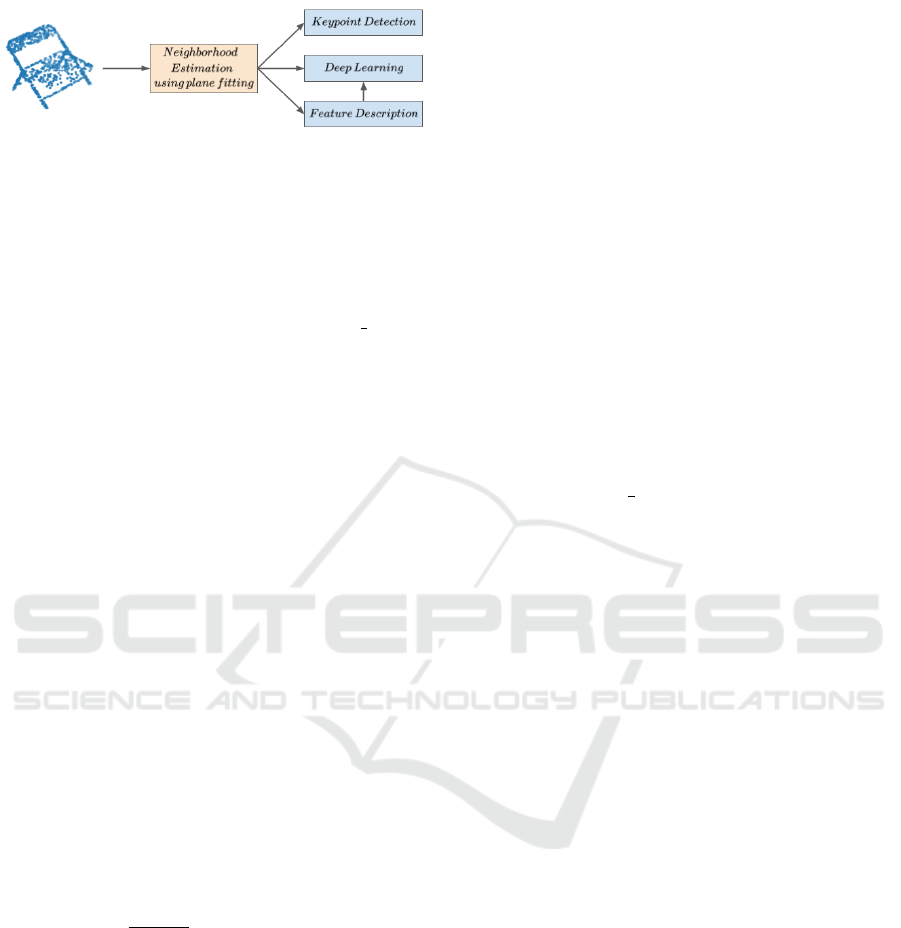
Figure 2: Point cloud neighborhood estimation and its vari-

ous applicability cases.

as the projection of points onto a plane with a constant

height and the assignment of points to the neighbor-

hood that are located within a circle of radius r.

r ∈ R, v

{

q | d(q, p) ≤ r

}

(1)

r ∈ R, v



q |



− q

)

+ (p

− q

)



≤ r



(2)

K-nearest neighborhoods is the most commonly uti-

lized similarity neighborhood. The k-nearest neigh-

borhood computes a similarity metric over all points

in the PCD. The top-k similar points are included in

the ﬁnal neighborhood. The Radial Basis Function

(RBF) kernel with a unit variance of the Euclidean

distance between the center point p and the surround-

ing points q is a regularly used similarity metric.

2.2 Plane Fitting

Following the selection of a neighborhood type and

parameters, relevant information is extracted from the

covariance matrix computed over the neighborhood’s

points. As described in equation (3), the covariance

matrix is a symmetric positive semi-deﬁnite matrix

computed using statistics over points within a neigh-

borhood v

centered at point p and parameterized by

r. The eigenvalues and eigenvectors of the covari-

ance matrix, recovered via eigenvalue decomposition

as seen in equation (4), are used to approximate the

ﬁtted plane.

Cov(v

) =

| − 1

∑

q∈v

(q − µ)

× (q − µ) (3)

λ ×Cov(v

) = λ × v (4)

2.3 Keypoints Detection

The majority of keypoints detection algorithms are

dependent on neighborhood estimation as an initial

processing step. Keypoints detection extracts points

with unique features within a local vicinity in a PCD.

ISS (Zhong, 2009) deﬁnes keypoints as points with

high 3D variation (smallest eigenvalue of the approx-

imate plane) within a local vicinity. To eliminate

any ambiguity in keypoints, ISS employs two pruning

techniques: points with equal eigenvalues omission

and resolution control. SURE (Fiolka et al., 2012) in-

vestigates the ratio between the approximated plane’s

maximum and minimum eigenvalues. Keypoints are

detected by applying a threshold operator on the in-

vestigated ratio.

MSV (Siritanawan et al., 2017) and MoPC

(Huang and You, 2012) apply multi-scale analysis by

ﬁtting neighborhoods of different scales to a point

of interest. The scales range between minimum and

maximum scales [s

min

, s

max

] and are increased with a

discrete step size. MSV keypoints are points whose

surface variation (smallest normalized eigenvalue of

the approximate plane) averaged over all scales is

higher than a certain threshold. MoPC, on the other

hand, selects keypoints based on principle curvature

(largest eigenvalue of the approximate plane). A point

at a given scale s

is considered a keypoint if it has the

largest principle curvature, when compared to both,

the same point at the previous scale s

n−1

and the sub-

sequent scale s

n+1

, and all its neighbors that lie within

a third of the scale

of the point.

2.4 Features Description

The detection of keypoints is followed by a descrip-

tion of their features in the encoding pipeline. The

aim of features description is to provide an extended

features vector for a more meaningful embedding of

PCD. (Vandapel et al., 2004) proposed a linear com-

bination of the eigenvalues of the estimated plane of

the keypoint, yielding an eigenvalue-based descriptor

which is resilient against rigid transformations. RSD

(Marton et al., 2010) models a radial relationship be-

tween a keypoint and its neighbors by the distance be-

tween them and the angle between their normals. The

ﬁnal descriptor is minimum and maximum radius at-

tained within a neighborhood. (Triebel et al., 2006)

utilized a 1D histogram of cosine angles between a

keypoint and its neighborhoods normal vectors as a

descriptor. Thrift (Flint et al., 2007) is another ap-

proach that uses 1D histograms of cosine angles, with

the angle deﬁned between normal vectors computed

on two different scales for the same keypoint neigh-

bor.

Spin Image (Johnson and Hebert, 1998) calculates

two geometric features (α, β) between a keypoint p

and its neighbor q by aid of the neighbor’s normal

vector n

. A 2D histogram over α, β of the keypoint

neighborhood is the proposed descriptor. The ap-

proach of PFH (Rusu et al., 2008b; Rusu et al., 2008a)

is similar to that of Spin Image. Given a keypoint p

and a pair of its neighbors, q

and q

, a darboux frame

is constructed based on the distance between the pair

VISAPP 2023 - 18th International Conference on Computer Vision Theory and Applications

584

and the normal vector of q

. Four geometric proper-

ties are derived using the darboux frame, and the ﬁnal

PFH descriptor is a 4D histogram that incorporates

these properties.

2.5 Deep Learning

The neighborhood estimation task has been used in a

number of deep learning modules. PointNet (Qi et al.,

2017a) is a pioneer work in deep learning on the raw

data of PCDs. Even though this network provided ad-

vancement in the ﬁeld and sparked huge interest in

learning from raw PCD, it lacked the ability to cap-

ture the correlation between neighboring points and

complex local geometries. Thus, (Qi et al., 2017b)

proposed PointNet++ to overcome this drawback by

hierarchical learning contextual information over a

PCD. PointNet++ samples a subset of points from a

PCD and groups points in a ﬁxed radius, ﬁxed neigh-

borhood parameter, around the sampled points using

a sampling and grouping layer. The grouped points

in the local neighborhood are processed using Point-

Net to extract useful information. DGCNN (Wang

et al., 2019) constructs a k-nearest neighbors graph

with ﬁxed K and uses an edge convolution layer to

learn from its constructed input. FoldingNet (Yang

et al., 2018) is a PCD auto-encoder architecture used

for reconstruction task. This architecture appends the

local covariance matrix of each point, calculated us-

ing a knn-neighborhood with K=16 as described in

equation (3), to the input feature vector. Both LPD-

Net (Liu et al., 2019) and its successor LPD-AE (Suo

et al., 2020) merge ten features that were retrieved

from the ﬁtted neighborhood with the input points

coordinates. The empirical results in the aforemen-

tioned papers and their analysis showed that select-

ing the optimal neighborhood size rather than a ﬁxed

one improved network performance and recall abil-

ity. However, a grid search with ﬁxed resolution

over neighborhood parameters was used, which has

the drawback of requiring a large amount of memory

and computing load. (Zhao et al., 2022) dedicated a

separate branch to extracting information from fea-

tures computed over a knn-neighborhoods with con-

stant size for all points. The retrieved features are cal-

culated using local frames constructed between a cen-

ter point p and its neighbor q, and are then fused with

extracted features from spatial information to form a

single descriptor. The addition of such features in-

creased the network’s robustness against rigid input

transformations.

2.6 Neighborhood Estimation Objective

Functions

(Demantk

e et al., 2011) identiﬁes two major issues

with selecting neighborhood parameters: it cannot be

chosen heuristically, and it cannot be constant over

the whole PCD. Instead, it should be directed by data

and tailored to varying densities and sizes of PCD lo-

cal geometries.

(Demantk

e et al., 2011) introduces two objective

functions for selecting neighborhood parameters. The

goal of such functions is to automate the selection of

the optimal neighborhood parameters for each point

in a PCD. Both objective functions are based on a

point’s dimensionality features, as described in (To-

shev et al., 2010). These features are calculated based

on eigenvalues ordered in descending order as de-

picted in equation (5), where a

, a

, and a

rep-

resent the degree of linearity, planarity, and scattering

exhibited by a point p when a neighborhood v param-

eterized by r is centered around p. The dimension-

ality label of a point p is the degree with the highest

value as provided in equation (6), where λ

≥ λ

represent the eigenvalues of the approximate plane in

descending order.

− λ

, a

− λ

, a

(5)

∗

) = argmax

d∈[1,3]

(6)

The ﬁrst objective function deﬁnes the optimal pa-

rameters as the parameters that minimize the Shannon

entropy of the dimensionality features within a neigh-

borhood, as described in equation (7, 8). The intuition

behind such an objective function is ﬁnding parame-

ters which favors a single dimensionality within the

neighborhood.

E(v

) = −a

ln(a

) − a

ln(a

) − a

ln(a

)

(7)

optimal

= arg min

E(v

) (8)

The other objective function supports picking a

neighborhood with the majority of points labeled with

the same dimensionality (homogeneous), as shown in

equations (9, 10).

S(v

) =

∑

q∈v

{

∗

)=d

∗

)

}

(9)

optimal

= arg max

S(v

) (10)

In the aforementioned work, both objective func-

tions were optimized using grid search with a prede-

ﬁned resolution bounded between (r

min

, r

max

). When

Point Cloud Neighborhood Estimation Method Using Deep Neuro-Evolution

585

compared to homogeneity-based criteria, the reported

results show that dimensionality-based entropy crite-

ria are more desirable since they can have a unique

solution per point and do not saturate.

An alternative entropy based objective function

is introduced in (Weinmann et al., 2015). Unlike

dimensionality-based functions, this function seeks to

reduce the Shannon entropy of the normalized eigen-

values, as proposed in equations (11, 12). The idea

behind such a function is to decrease noise and uncer-

tainty in the selected neighborhood eigenvalues.

+ λ

(11)

E(v

) = −ε

ln(ε

) − ε

ln(ε

) − ε

ln(ε

) (12)

3 METHODOLOGY

As discussed in Section 2 and illustrated in ﬁgure (2),

explicit neighborhood estimation is an essential pre-

processing step for efﬁcient PCD analysis. In this

work, we propose a pipeline for explicit and opti-

mal neighborhood estimation. The pipeline doesn’t

require supervision or access to ground truth infor-

mation such as normal vectors or curvatures. It is

worth mentioning that the estimated neighborhoods

are task-agnostic, with desirable properties due to the

choice of the objective function. Additionally, the

neighborhood is designed with low memory and com-

putation footprint to accelerate the task signiﬁcantly.

A pipeline for neighborhood estimation that is

both memory and computationally efﬁcient is lacking

in the literature, since only grid search with a ﬁxed

resolution was used to minimize objective functions

addressed in Section 2.6. The two objective functions

depicted in equations (7, 12) are used for automated

neighborhood estimation in this work. The third ob-

jective function presented in equation (9) is disre-

garded as it has a combinatorial nature, and empirical

results reported in (Demantk

e et al., 2011) demon-

strate that it performs poorly when compared to the

other two. In this work, we focus on increasing the

task efﬁciency by learning the optimal neighborhood

parameter choice over a small subset of points from

a PCD driven by the aforementioned objective func-

tions and then generalizing this learning across the re-

maining points.

This work adopts and modiﬁes Deep Neuro-

Evolution (Salimans et al., 2017) as the building block

of the proposed pipeline. To the best of our knowl-

edge, this work is the ﬁrst in modifying Deep Neuro-

Evolution as a parameter estimation module. Deep

Neuro-Evolution (Such et al., 2017) is a non-gradient-

based alternative to deep reinforcement learning and

is described as the successor to evolution strategies in-

troduced in (Salimans et al., 2017). Evolution Strate-

gies (ES) is a gradient-based deep evolution technique

that produces results comparable to Q-learning and

policy gradient approaches (Salimans et al., 2017).

ES evaluates a network at a number of mutations gen-

erated by random noise. A gradient approximated

by a modiﬁed ﬁnite-difference operation is used to

update the network parameters. The success of ES

sparked interest in developing an entirely gradient-

free technique based on evolutionary algorithms that

can scale effectively as a deep reinforcement learn-

ing alternative, leading to the formulation of Deep

Neuro-Evolution. In comparison to deep reinforce-

ment learning and ES, Deep Neuro-Evolution has

a sizable advantage in the neighborhood estimation

problem and requires far less memory compared to

reinforcement learning because it does not require

state representation or buffer memory. Additionally,

since Deep Neuro-Evolution does not require back-

propagation, it requires less computational effort than

approaches as in (Such et al., 2017). Furthermore, it

can also be used in a distributed manner over multiple

threads.

Preliminaries. Deep Neuro-Evolution is a variant

of the standard genetic algorithm, in which each in-

dividual (genotype) is a neural network. A mutation

function ψ, network initialization method φ, and ﬁt-

ness function F are all required by the algorithm in

addition to the number of individuals in each gener-

ation, the number of generations, and the number of

top T performing individuals to keep for next gen-

erations. The mutation function ψ modiﬁes the net-

work’s weights to generate a new individual, while

the network initialization φ provides a deterministic

method for creating the initial network’s weights. Fi-

nally, the ﬁtness function is utilized to assess each in-

dividual’s performance.

Our proposed Deep Neuro-Evolution uses a shal-

low version of PointNet (Qi et al., 2017a) as an indi-

vidual, which uses blocks of Multi-Layer Perceptron

(MLP) and Relu Nonlinearity to process each point

in the input individually. In this work, the shallow

network has two PointNet blocks, thus having very

few learnable parameters, decreasing the computation

load. The second block’s output is collapsed by max

pooling, as it is a permutation invariant function due

to its symmetric nature, into a global description. A

linear layer is added after the global description vec-

tor to obtain the network’s ﬁnal output. The network

input is the PCD centered around the point of interest

p for which the neighborhood is estimated. More-

over, the network computation can be enhanced by

VISAPP 2023 - 18th International Conference on Computer Vision Theory and Applications

586

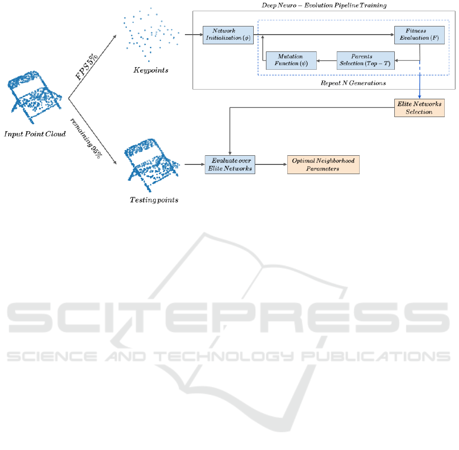
Figure 3: Pipeline overview. A subset of points is sampled using FPS, which are used to train the proposed pipeline. The

proposed pipeline searches for the Elite Networks for the neighborhood estimation task. The Elite Networks are subsequently

used to estimate parameters of the remaining points.

only taking a sufﬁcient subset of the PCD around the

point of interest. The network output is the neigh-

borhood parameterization and is subjected to a tanh

non-linearity to constrain it to the range [-1, 1], after

which it is remapped to fulﬁl the chosen parameter

limits.

Deep Neuro-Evolution searches for the ﬁttest in-

dividual (Elite) among those created over G genera-

tions. The ﬁtness of each individual in estimating a

neighborhood for a center point p is evaluated using

our novel ﬁtness function proposed in equation (13).

The ﬁtness function’s ﬁrst term is in charge of pro-

moting neighborhood parameter selection that mini-

mizes neighborhood entropy and represents the dif-

ference between the maximum Shannon entropy of

a neighborhood deﬁned over three random variables

(x, y, z), which is equal to ln (3), and the neighborhood

entropy obtained with network estimated parameters

. As a consequence, the ﬁttest parameter choice is

the one with the lowest entropy, as required by equa-

tion (8). Furthermore, this term is independent of the

entropy function employed, and it can be calculated

using either the eigen entropy or the dimensionality

entropy stated in equations (7, 12). The second term

of equation (13) is responsible for penalizing neigh-

borhoods with less than two points in the neighbor-

hood, since this is a trivial solution and doesn’t pro-

vide any tractable information about the center point

F(θ

) =



ln(3) − E(v

)



+ ln(3) × 1

(13)

In the initial generation, N − 1 individuals are

created with randomly initialized weights using the

Xavier uniform initialization (Glorot and Bengio,

2010). The beneﬁt of this initialization is that the net-

work is not biased towards any single region in the

search space, but instead has a uniform distribution of

output over the whole search space.

For subsequent generations, one of the top T -

performing parents is uniformly sampled at random.

The sampled parent weights are mutated by applying

an additive Gaussian noise regulated by a hyperpa-

rameter σ as seen in equation (14), to generate a new

individual which explores a slightly different region

in the search space. The hyperparameter σ controls

how dispersed the new individual is from its parent

in the search space. A high sigma value causes sig-

niﬁcant jumps in the search process, whereas a low

sigma causes the search to be localized and limited to

a certain region of the search space. As a result, the

initial value of σ is obtained empirically during exper-

iments, and σ decays at a linear rate every generation,

allowing the search to be more localized in the ﬁttest

areas of the search space as the number of generations

increases. This concept is parallel to the exploration-

exploitation trade-off in reinforcement learning (Sali-

mans et al., 2017).

ε ∼ N (0,I)

= ψ (θ

n−1

, ε) = θ

n−1

+ σ × ε

(14)

Each mutated individual performance is evaluated

using ﬁtness function F. Consequently, the generated

individuals are ordered in a descending manner based

on their ﬁtness score. The set of elite candidates is es-

tablished through truncation selection, which involves

picking the top T -performing parents. The elite indi-

Point Cloud Neighborhood Estimation Method Using Deep Neuro-Evolution

587

vidual, the best performing one globally during the

search process thus far, is updated by comparison to

the maximum argument over the candidate set and ap-

pended to the candidate set if not already a member.

The elite individual (network) with the ﬁttest neigh-

borhood parameters is returned as the algorithm out-

put once all generations have been generated. This

elite individual can be utilized in estimating neighbor-

hood parameters for other points that exhibit similar

geometric and spatial properties.

Even though the adapted Deep Neuro-evolution

approach has low memory and processing, it is in-

efﬁcient for estimating neighborhood parameters per

point, especially on large scale PCDs with millions

of points. It is more efﬁcient to learn the parame-

ter search using Deep Neuro-evolution over a small

sample of points, 5% of the points in the PCD, and

then applying the learned search over the remaining

95% unseen points in the PCD. The overall pipeline

pseudocode is illustrated in algorithm 1. It should be

highlighted that pipeline efﬁciency in both the Deep

Neuro-evolution (lines 2–5) and the elite networks’

evaluation (lines 6–14) stages are further improved by

utilizing a relevant subset of points as the network in-

put instead of the whole PCD e.g. the points included

within the neighborhood deﬁned by the maximum pa-

rameter. Additionally, a visual clariﬁcation of the pro-

posed pipeline can be seen in ﬁgure (3).

Different sampling techniques have been pro-

posed in the literature to extract keypoints from a PCD

as discussed in Section 2.3. However, since most

of these approaches rely on neighborhood estimation,

using them in the proposed pipeline is contradictory.

Whereas, random sampling and FPS were described

as effective keypoints sampling alternatives for PCD

in (Varga et al., 2021; Qi et al., 2017b) respectively.

Random sampling draws a subset of points from a

PCD uniformly at random. FPS, on the other hand,

is an iterative sampling technique that starts with a

random point as a seed and samples the PCD’s far-

thest point from the previously sampled seed as the

new seed in an iterative manner. In this work, FPS

is preferable since it captures the PCD structure and

summarizes its details in a few points, whereas ran-

dom sampling loses shape details and rough struc-

ture, and can easily hinder the pipeline performance,

as shown by the example on ﬁgure (4c).

Classical multi-scale shape analysis (Demantk

et al., 2011) proposes multiple analysis scales ﬁxed

for all points, which are not tailored by the data. Our

pipeline is more effective than multi-scale analysis

since it requires less computational power and di-

rectly extracts a single optimal value for each param-

eter, which can then be used for the precise estima-

Algorithm 1: The proposed pipeline Pseudocode.

Require: mutation function ψ, population size N,

number of selected individuals T , number of gen-

erations G, network initialization routine φ, ﬁt-

ness function F, point cloud P

1: sample 5% of the total points in P as keypoints Q

using FPS as in line with (Qi et al., 2017b)

2: for each keypoint q in Q do

3: elite ← Deep Neuro-Evolution(ψ, N, T , G, φ,

F, P centered around q) as in line with (Such

et al., 2017)

4: Elite networks ← Elite networks ∪ elite

5: end for

6: for each remaining point p in P \ Q do

7: for each elite in Elite networks do

8: neighborhood parameters ← elite (P cen-

tered around p)

9: neighborhood ﬁtness ← F (neighborhood

parameters)

10: if best ﬁtness < neighborhood ﬁtness then

11: best ﬁtness ← neighborhood ﬁtness

12: optimal parameters ← neighborhood pa-

rameters

13: end if

14: end for

15: Per-point parameters ← Per-point parameters

∪ optimal parameters

16: end for

17: return Per-point parameters

tion of a center point characteristics like normal vec-

tors and curvatures and employed in clustering frame-

works like the region growing algorithm (Rabbani

et al., 2006). Furthermore, our pipeline is easily ex-

tensible as an enhanced multi-scale analysis approach

by altering the pipeline’s output to be the top − k

elite individuals for each point in the keypoints, hence

strengthening the multi-scale analysis by selecting in-

formative scales based on geometric and spatial prop-

erties of points rather than a pre-deﬁned set identical

for all points.

It is essential to emphasize, that the proposed

pipeline is an unsupervised approach guided by a

novel objective function for hard assignment of lo-

cal neighborhoods. There are other approaches that

focus on soft assignment of neighborhoods, such as

(Ben-Shabat et al., 2019; Zhou et al., 2021a; Ben-

Shabat and Gould, 2020; Zhu et al., 2021; Zhou et al.,

2021b). The soft assignment is established for a cen-

ter point by learning weights over neighboring points

on a rather big neighborhood size ﬁxed for all cen-

ter points. However, the aforementioned approaches

are trained in a supervised manner to minimize nor-

mal estimation loss given its ground truth and uti-

VISAPP 2023 - 18th International Conference on Computer Vision Theory and Applications

588

(a) Input point cloud.

(b) Output point cloud using FPS.

sampling.

Figure 4: Output point clouds of a chair class from different sampling techniques. The output illustrates that FPS is favorable

than random sampling as it has the ability to summaries a point cloud in few points while maintaining its structure.

lize a large patch of points around a center point

without explicit extraction of neighborhood parame-

ters. Whereas, our method explicitly extracts neigh-

borhood parameters and is task-agonistic such that

the neighborhood has desired properties that can be

later ﬁne-tuned for speciﬁc tasks such as the ones dis-

cussed in Section 2, which are out of the scope of this

research. Moreover, in (Zhou et al., 2021b), one of

the best-performing networks on supervised normal

estimation, authors reported that utilization of a ﬁrst-

order jet ﬁtting, equivalent to the plane ﬁtting used

in our work, and top − k selection strategy enhances

normal estimation results. The top − k selection only

uses information from the top − k critical points for

ﬁtting, however, it is manually set and ﬁxed for all

points. In our paper, we provided a method for the

dynamic setting of the k parameter of an unweighted

ﬁtting approach. Furthermore, our work can directly

beneﬁt pre-processing steps of other approaches such

as (Yang et al., 2018; Suo et al., 2020; Liu et al.,

2019), which the aforementioned approaches cannot

contribute to. Finally, the proposed approach has con-

siderably fewer learnable parameters than all other

networks and can be used to estimate parameters for a

single PCD without any pre-training. For future work,

it is planned to integrate both jet ﬁtting and weighted

neighborhoods in our pipeline while keeping its unsu-

pervised setting.

4 EVALUATION

4.1 Dataset

In this work, ModelNet-10 dataset is used for the eval-

uation purposes of the proposed neighborhood esti-

mation pipeline. ModelNet-10 is a benchmark for

3D object classiﬁcation and retrieval published by

Princeton University in (Wu et al., 2015). The dataset

contains, 4899 CAD-generated meshes stored in Ob-

ject File Format (OFF), which are divided into 3991

meshes for training and 908 meshes for testing pur-

poses. Moreover, it is well known in the research

community since it is a well-structured dataset with

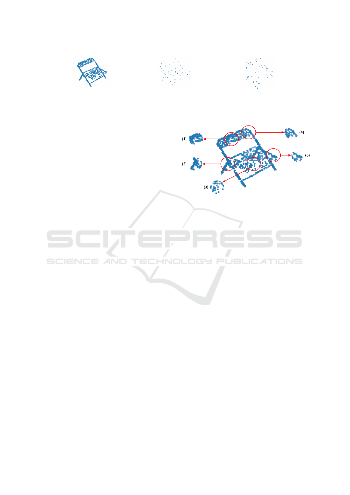
Figure 5: Different examples of points irregularity and com-

plex features that require the adaptation of the neighbor-

hood parameters.

pre-aligned clean shapes sampled from several cate-

gories. Currently, the dataset has ten classes: bathtub,

bed, chair, desk, dresser, monitor, nightstand, sofa,

table, and toilet. An output PCD is generated by

randomly sampling points from the CAD-generated

mesh’s triangular faces, which enforces the existence

of irregularities in the PCD. The sampled points are

normalized and ﬁtted into a bounding box between

[−1, 1]. Even though ModelNet 10 dataset is a clean

and aligned dataset, it contains a variety of objects

with complex geometries that necessitate the adapta-

tion of the neighborhood parameters. Figure (5) illus-

trates an example of a PCD from class chair. Different

regions with less dense points distribution and irreg-

ular nature are highlighted in ﬁgure (5: sub-ﬁgures

2 and 5). Additionally, these examples clarify that

edges, corners and other ﬁne details require adapta-

tion of the neighborhood parameters to be captured

correctly compared to points belonging to coarser fea-

tures such as the seat or the back of the chair as de-

picted in ﬁgure (5: sub-ﬁgures 3, 1, 4 respectively).

4.2 Evaluation Metrics

A k-nearest neighborhood using RBF kernel of Eu-

clidean distance as a similarity metric and constant

size K = 30 is utilized as a baseline against which

this work was evaluated, which is the standard ap-

proach for ﬁtting a neighborhood to the ModelNet-

10 dataset (Qi et al., 2017b; Wang et al., 2019). The

Point Cloud Neighborhood Estimation Method Using Deep Neuro-Evolution

589

primary evaluation metrics in this work are: a) the

minimization of eigen entropy and b) minimization

of dimensionality entropy objective functions for-

mulated in equations (7, 12) respectively. These two

objective functions are reviewed in the literature (De-

mantk

e et al., 2011; Weinmann et al., 2015), where

achieving lower entropy implies the choice of more

optimal parameters. The entropy minimization evalu-

ations demonstrate the pipeline’s efﬁciency of its op-

timization characteristics and ability to generalize for

learning over only a small subset of points in the PCD.

Despite the fact that neighborhood estimation is

explicitly correlated to the normal estimation task for

a PCD, we, additionally, use our pipeline to inves-

tigate the impact of optimal neighborhood selection

on such a task . In our work, the normal vector at

a point in the PCD is approximated by the eigenvec-

tor of the smallest eigenvalue of the estimated neigh-

borhood at the point. Besides, the unoriented angle

similarity and the proportion of good points (PGP) as

introduced in (Wang and Prisacariu, 2020) are used

to assess the quality of the normal estimation. As

seen in equation (16), the unoriented angle similarity

measures the similarity between the estimated normal

vector ˆn and a ground truth normal vector n, which

is the normal vector at the triangular face from which

the point is sampled. The unoriented angle similarity

calculates the similarity by ﬁrst computing the angle β

between ˆn and n as in equation (15), and then normal-

izing the angle β by the maximum angular difference

max

, which in this case is set to 90

◦

. The percent-

age of good points (PGP) is another evaluation metric

for normal estimation tasks, where PGP

denotes the

percentage of points having a normal estimation er-

ror of less than α, as seen in equation (17). Crucially,

we assess the proposed pipeline over normal estima-

tion task only since it has the aforementioned metrics

of evaluation, whereas keypoint detection and fea-

ture description have no quantitative evaluations and

are instead evaluated qualitatively which is inconclu-

sive. Furthermore, we compare our pipeline against

the classical Principal Components Analysis (PCA),

as discussed in (Demantk

e et al., 2011), since it com-

putes normal vectors in an unsupervised manner and

our pipeline serves as a pre-processing step for choos-

ing meaningful parameters to be used by PCA.

β = arccos





ˆn · n

ˆn





(15)

similarity (β) = 1 −

max

(16)

PGP

∑

a∈P

<α

(17)

4.3 Training Setting

The implementation of the proposed pipeline is real-

ized in Python 3.9 and PyTorch 1.10.0 without uti-

lizing GPUs or parallel threading. Even though a

GPU-enabled implementation is available and a par-

allel threading version of the pipeline, in which dif-

ferent keypoints can be deployed on multiple threads,

can be adapted in a straightforward manner for faster

execution. The lightweight PointNet blocks have 16

output features each, where the network weights are

initialized using Xavier uniform initialization and the

biases are set to 0.01. The hyperparameter σ of the

mutation function, as described in equation (14), is

set to 0.3 and decay linearly with 0.05 at each genera-

tion. Given each keypoint, the modiﬁed deep Neuro-

Evolution runs for 5 generations with a population

size of 50 individuals and keeps the top 20 perform-

ing individuals at each generation to act as parents of

the subsequent generation.

4.4 Results

Table 1 illustrates the eigen and dimensionality en-

tropy produced by our pipeline in different neighbor-

hood types, compared to the classical baseline. This

table is dedicated to the results of the training and test-

ing points. Training points are points sampled with

FPS and passed in an unsupervised training manner

to Deep Neuro-evolution. A total of 1028 points are

sampled from each mesh, however, only 51 points are

used for training. The ﬁndings indicate that indepen-

dent of the neighborhood type, our proposed pipeline

attains lower (better) entropy values compared to the

baseline. The test points are the 95% remaining points

that were not included in the pipeline training. Re-

sults show that the pipeline has a good generaliza-

tion performance over the unseen points. These re-

sults support our hypothesis that when directed by the

novel ﬁtness function provided in equation (13), an

intelligent sampling approach (FPS) and Deep Neuro-

Evolution as a learning algorithm an effective and

novel pipeline for neighborhood estimation is pro-

posed.

Table 2 illustrates normal estimation results under

unoriented angle similarity and PGP metrics. PGP

is investigated at three distinct α levels in order to

offer a more comprehensive view of our approach’s

performance. The table draws a comparison between

our proposed pipeline trained with different types of

neighborhoods and optimizing either dimensionality

or eigenvalues entropy objective functions and the

baseline. Moreover, it provides results over training

points gathered with a sample percentage as discussed

VISAPP 2023 - 18th International Conference on Computer Vision Theory and Applications

590

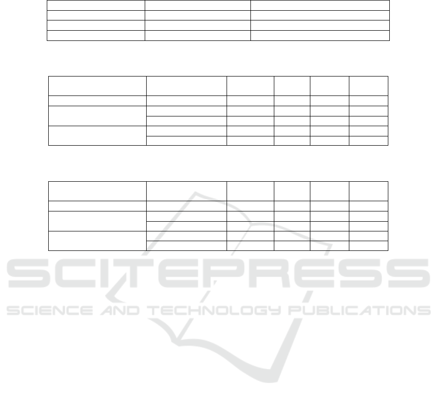
Table 1: Entropy results on training/testing points between classical baseline vs. adaptable neighborhoods, estimated using

our pipeline for both spherical and K nearest neighborhoods. The lower values indicate better performance.

Neighborhood Type Eigen Entropy (train / test) Dimensionality Entropy (train / test)

Classic 0.8279 / 0.8279 0.8443 / 0.8436

Spherical Neighborhood 0.7365 / 0.7231 0.645 / 0.6456

K nearest neighbors 0.7185 / 0.7127 0.6431 / 0.6295

Table 2: Normal estimation results on training points between classical baseline vs. adaptable neighborhoods estimated using

our pipeline for both spherical and K nearest neighborhoods. The higher values indicate better performance.

Neighborhood Type Objective Function

Angular

Similarity

PGP 5 PGP 10 PGP 30

Classic N/A 0.6769 0.2029 0.3380 0.6140

Spherical Neighborhood

Dimension Entropy 0.6849 0.2542 0.3839 0.6211

Eigen Entropy 0.6953 0.2771 0.4093 0.6421

K nearest neighbors

Dimension Entropy 0.6856 0.2563 0.3865 0.6213

Eigen Entropy 0.6856 0.2563 0.3865 0.6213

Table 3: Normal estimation results on test points between classical baseline vs. adaptable neighborhoods estimated using our

pipeline for both spherical and K nearest neighborhoods. The higher values indicate better performance.

Neighborhood Type Objective Function

Angular

Similarity

PGP 5 PGP 10 PGP 30

Classic N/A 0.6778 0.2038 0.3384 0.6169

Spherical Neighborhood

Dimension Entropy 0.6880 0.2550 0.3849 0.6258

Eigen Entropy 0.6981 0.2804 0.4127 0.6463

K nearest neighbors

Dimension Entropy 0.6773 0.2070 0.3424 0.6167

Eigen Entropy 0.6773 0.2070 0.3424 0.6167

earlier. The results reveal that optimal neighborhood

selection has a positive inﬂuence on the normal es-

timation results. The proposed pipeline outperforms

the classical approach by a signiﬁcant margin, with

the spherical neighborhood trained by eigen entropy

as the objective function being the best-performing

setting. When compared to the baseline, this set-

ting provides a 2% improvement in unoriented angu-

lar similarity and a 4% improvement in PGP on aver-

age.

The results are extended in Table 3 to include un-

seen test points. The results conﬁrm that the spherical

neighborhood has the highest capacity to generalize

across unseen data. Hence, we can conclude based on

both Tables 2, 3 that the best ﬁtting choice for nor-

mal estimation is a symmetric (spherical) neighbor-

hood with an equivalent dispersion in all directions

selected to minimize eigen entropy.

5 FUTURE WORK

For future work, it should be investigated whether the

learned neighborhood estimation can generalize not

only on points in the same PCD but also on points

from different PCDs that have similar structure or be-

long to the same class. The proposed approach may

additionally be validated on other datasets similar to

ModelNet such as PCPNet (Guerrero et al., 2018) and

is planned to be addressed in future works. Addition-

ally, the pipeline should be extended and validated on

large-scale PCDs with millions of points. Our hypoth-

esis is that employing our pipeline will have a positive

effect, as empirical results provided in LPDNet (Liu

et al., 2019) have shown that an optimal neighborhood

selection has a positive effect on the network perfor-

mance, yet the grid search used in this work has a

large memory and computation overhead. Different

sampling techniques should be investigated on a large

scale PCDs. One good candidate is using spatial clus-

tering over a PCD to create coarse regions of interest,

followed by FPS over the clustered areas. The ini-

tial clustering stage has the advantage of providing

an approximate count of the number of objects in the

scene, which helps FPS to sample points that summa-

rize the structure of the different objects. Finally, the

design of neighborhood selection heuristics and ob-

jective functions is still a work in progress, which can

be tailored to reduce errors in neighborhood attributes

like the normal vector.

6 CONCLUSION

In this work, we proposed a novel and efﬁcient

pipeline for neighborhood estimation given PCDs,

Point Cloud Neighborhood Estimation Method Using Deep Neuro-Evolution

591

which is a major challenge for both machine learning

and deep learning methods. The proposed pipeline

uses a modiﬁcation of Deep Neuro-Evolution as a

learning module and FPS for intelligent sampling.

Besides, a novel ﬁtness function is proposed to evalu-

ate the quality of each individual to reveal the elite

solution by applying random mutations of the net-

work parameters for a pre-determined number of gen-

erations. To further improve pipeline efﬁciency, we

propose to use only 5% of sampled points and uti-

lize them for the learning phase, while the remain-

ing 95% of points’ neighborhood is used to estimate

the pipeline generalization performance. In compar-

ison to the baseline, the pipeline was able to reduce

entropy values regardless of the neighborhood type.

Furthermore, the pipeline has a positive impact on

the normal estimation problem, with spherical neigh-

borhoods that optimize eigenvalues entropy deliver-

ing the best results.

REFERENCES

Bello, S. A., Yu, S., Wang, C., Adam, J. M., and Li, J.

(2020). Deep learning on 3d point clouds. Remote

Sensing, 12(11):1729.

Ben-Shabat, Y. and Gould, S. (2020). Deepﬁt: 3d surface

ﬁtting via neural network weighted least squares. In

European conference on computer vision, pages 20–

34. Springer.

Ben-Shabat, Y., Lindenbaum, M., and Fischer, A. (2019).

Nesti-net: Normal estimation for unstructured 3d

point clouds using convolutional neural networks. In

Proceedings of the IEEE/CVF Conference on Com-

puter Vision and Pattern Recognition, pages 10112–

10120.

Chai, J., Zeng, H., Li, A., and Ngai, E. W. (2021). Deep

learning in computer vision: A critical review of

emerging techniques and application scenarios. Ma-

chine Learning with Applications, 6:100134.

Cirujeda, P., Mateo, X., Dicente, Y., and Binefa, X. (2014).

Mcov: a covariance descriptor for fusion of texture

and shape features in 3d point clouds. In 2014 2nd In-

ternational Conference on 3D Vision, volume 1, pages

551–558. IEEE.

Demantk

e, J., Mallet, C., David, N., and Vallet, B. (2011).

Dimensionality based scale selection in 3d lidar point

clouds. In Laserscanning.

Eldar, Y., Lindenbaum, M., Porat, M., and Zeevi, Y. Y.

(1994). The farthest point strategy for progressive im-

age sampling. Proceedings of the 12th IAPR Inter-

national Conference on Pattern Recognition, Vol. 2 -

Conference B: Computer Vision & Image Processing.

(Cat. No.94CH3440-5), pages 93–97 vol.3.

Fiolka, T., St

uckler, J., Klein, D. A., Schulz, D., and

Behnke, S. (2012). Sure: Surface entropy for dis-

tinctive 3d features. In International Conference on

Spatial Cognition, pages 74–93. Springer.

Flint, A., Dick, A., and Van Den Hengel, A. (2007). Thrift:

Local 3d structure recognition. In 9th Biennial Con-

ference of the Australian Pattern Recognition Society

on Digital Image Computing Techniques and Applica-

tions (DICTA 2007), pages 182–188. IEEE.

Glorot, X. and Bengio, Y. (2010). Understanding the difﬁ-

culty of training deep feedforward neural networks. In

Proceedings of the thirteenth international conference

on artiﬁcial intelligence and statistics, pages 249–

256. JMLR Workshop and Conference Proceedings.

Guerrero, P., Kleiman, Y., Ovsjanikov, M., and Mitra, N. J.

(2018). Pcpnet learning local shape properties from

raw point clouds. In Computer Graphics Forum, vol-

ume 37, pages 75–85. Wiley Online Library.

Huang, J. and You, S. (2012). Point cloud matching based

on 3d self-similarity. In 2012 IEEE Computer Society

Conference on Computer Vision and Pattern Recogni-

tion Workshops, pages 41–48. IEEE.

Johnson, A. and Hebert, M. (1998). Surface matching for

object recognition in complex 3-d scenes. to appear in.

Image and Vision Computing.

Lazaros, N., Sirakoulis, G. C., and Gasteratos, A. (2008).

Review of stereo vision algorithms: From software to

hardware. International Journal of Optomechatronics,

2:435 – 462.

Liu, Z., Zhou, S., Suo, C., Yin, P., Chen, W., Wang, H., Li,

H., and Liu, Y.-H. (2019). Lpd-net: 3d point cloud

learning for large-scale place recognition and envi-

ronment analysis. In Proceedings of the IEEE/CVF

International Conference on Computer Vision, pages

2831–2840.

Marton, Z.-C., Pangercic, D., Blodow, N., Kleinehellefort,

J., and Beetz, M. (2010). General 3d modelling of

novel objects from a single view. In 2010 ieee/rsj in-

ternational conference on intelligent robots and sys-

tems, pages 3700–3705. IEEE.

Ming, Y., Meng, X., Fan, C., and Yu, H. (2021). Deep

learning for monocular depth estimation: A review.

Neurocomputing, 438:14–33.

Qi, C. R., Su, H., Mo, K., and Guibas, L. J. (2017a). Point-

net: Deep learning on point sets for 3d classiﬁcation

and segmentation. In Proceedings of the IEEE con-

ference on computer vision and pattern recognition,

pages 652–660.

Qi, C. R., Yi, L., Su, H., and Guibas, L. J. (2017b). Point-

net++: Deep hierarchical feature learning on point sets

in a metric space. Advances in neural information pro-

cessing systems, 30.

Rabbani, T., Van Den Heuvel, F., and Vosselmann, G.

(2006). Segmentation of point clouds using smooth-

ness constraint. International archives of photogram-

metry, remote sensing and spatial information sci-

ences, 36(5):248–253.

Royo, S. and Ballesta-Garcia, M. (2019). An overview of

lidar imaging systems for autonomous vehicles. Ap-

plied Sciences, 9:4093.

Rusu, R. B., Blodow, N., Marton, Z. C., and Beetz, M.

(2008a). Aligning point cloud views using persistent

feature histograms. In 2008 IEEE/RSJ international

VISAPP 2023 - 18th International Conference on Computer Vision Theory and Applications

592

conference on intelligent robots and systems, pages

3384–3391. IEEE.

Rusu, R. B., Marton, Z. C., Blodow, N., and Beetz, M.

(2008b). Persistent point feature histograms for 3d

point clouds. In Proc 10th Int Conf Intel Autonomous

Syst (IAS-10), Baden-Baden, Germany, pages 119–

128.

Salimans, T., Ho, J., Chen, X., Sidor, S., and Sutskever,

I. (2017). Evolution strategies as a scalable al-

ternative to reinforcement learning. arXiv preprint

arXiv:1703.03864.

Siritanawan, P., Prasanjith, M. D., and Wang, D. (2017).

3d feature points detection on sparse and non-uniform

pointcloud for slam. In 2017 18th International Con-

ference on Advanced Robotics (ICAR), pages 112–

117. IEEE.

Such, F. P., Madhavan, V., Conti, E., Lehman, J., Stanley,

K. O., and Clune, J. (2017). Deep neuroevolution: Ge-

netic algorithms are a competitive alternative for train-

ing deep neural networks for reinforcement learning.

arXiv preprint arXiv:1712.06567.

Suo, C., Liu, Z., Mo, L., and Liu, Y. (2020). Lpd-ae: la-

tent space representation of large-scale 3d point cloud.

IEEE Access, 8:108402–108417.

Toshev, A., Mordohai, P., and Taskar, B. (2010). Detecting

and parsing architecture at city scale from range data.

In 2010 IEEE Computer Society Conference on Com-

puter Vision and Pattern Recognition, pages 398–405.

IEEE.

Triebel, R., Kersting, K., and Burgard, W. (2006). Robust

3d scan point classiﬁcation using associative markov

networks. In Proceedings 2006 IEEE International

Conference on Robotics and Automation, 2006. ICRA

2006., pages 2603–2608. IEEE.

Vandapel, N., Huber, D. F., Kapuria, A., and Hebert, M.

(2004). Natural terrain classiﬁcation using 3-d ladar

data. In IEEE International Conference on Robotics

and Automation, 2004. Proceedings. ICRA’04. 2004,

volume 5, pages 5117–5122. IEEE.

Varga, D., Szalai-Gindl, J. M., Formanek, B., Vaderna, P.,

Dobos, L., and Laki, S. (2021). Template matching

for 3d objects in large point clouds using dbms. IEEE

Access, 9:76894–76907.

Wang, Y., Sun, Y., Liu, Z., Sarma, S. E., Bronstein, M. M.,

and Solomon, J. M. (2019). Dynamic graph cnn

for learning on point clouds. Acm Transactions On

Graphics (tog), 38(5):1–12.

Wang, Z. and Prisacariu, V. A. (2020). Neighbourhood-

insensitive point cloud normal estimation network.

arXiv preprint arXiv:2008.09965.

Weinmann, M., Jutzi, B., and Mallet, C. (2014). Seman-

tic 3d scene interpretation: A framework combining

optimal neighborhood size selection with relevant fea-

tures. ISPRS Annals of the Photogrammetry, Remote

Sensing and Spatial Information Sciences, 2(3):181.

Weinmann, M., Schmidt, A., Mallet, C., Hinz, S., Rotten-

steiner, F., and Jutzi, B. (2015). Contextual classiﬁ-

cation of point cloud data by exploiting individual 3d

neigbourhoods. ISPRS Annals of the Photogramme-

try, Remote Sensing and Spatial Information Sciences

II-3 (2015), Nr. W4, 2(W4):271–278.

Wu, Z., Song, S., Khosla, A., Yu, F., Zhang, L., Tang, X.,

and Xiao, J. (2015). 3d shapenets: A deep representa-

tion for volumetric shapes. In Proceedings of the IEEE

conference on computer vision and pattern recogni-

tion, pages 1912–1920.

Yang, Y., Feng, C., Shen, Y., and Tian, D. (2018). Fold-

ingnet: Point cloud auto-encoder via deep grid defor-

mation. In Proceedings of the IEEE conference on

computer vision and pattern recognition, pages 206–

215.

Zhao, C., Yang, J., Xiong, X., Zhu, A., Cao, Z., and Li,

X. (2022). Rotation invariant point cloud analysis:

Where local geometry meets global topology. Pattern

Recognition, 127:108626.

Zhong, Y. (2009). Intrinsic shape signatures: A shape de-

scriptor for 3d object recognition. In 2009 IEEE 12th

international conference on computer vision work-

shops, ICCV Workshops, pages 689–696. IEEE.

Zhou, J., Jin, W., Wang, M., Liu, X., Li, Z., and Liu, Z.

(2021a). Improvement of normal estimation for point-

clouds via simplifying surface ﬁtting. arXiv preprint

arXiv:2104.10369.

Zhou, J., Jin, W., Wang, M., Liu, X., Li, Z., and Liu,

Z. (2021b). Improvement of normal estimation for

pointclouds via simplifying surface ﬁtting. ArXiv,

abs/2104.10369.

Zhu, R., Liu, Y., Dong, Z., Wang, Y., Jiang, T., Wang, W.,

and Yang, B. (2021). Adaﬁt: Rethinking learning-

based normal estimation on point clouds. In Pro-

ceedings of the IEEE/CVF International Conference

on Computer Vision, pages 6118–6127.

Point Cloud Neighborhood Estimation Method Using Deep Neuro-Evolution

593