Deep Learning Model Selection With Parametric Complexity Control

Olga Grebenkova

1,2 a

, Oleg Bakhteev

1,3 b

and Vadim Strijov

3 c

Moscow Institute of Physics and Technology (MIPT), Russia

Skolkovo Institute of Science and Technology (Skoltech), Russia

FRC CSC RAS, Russia

Keywords:

Model Complexity Control, Hypernetworks, Variational Model Optimization, Bayesian Inference.

Abstract:

The paper is devoted to deep learning model complexity. It is estimated by Bayesian inference and based

on a computational budget. The idea of the proposed method is to represent deep learning model parameters

in the form of hypernetwork output. A hypernetwork is a supplementary model which generates parameters

of the selected model. This paper considers the minimum description length from a Bayesian point of view.

We introduce prior distributions of deep learning model parameters to control the model complexity. The

paper analyzes and compares three types of regularization to deﬁne the parameter distribution. It infers and

generalizes the model evidence as a criterion that depends on the required model complexity. Finally, it

analyzes this method in the computational experiments on the Wine, MNIST, and CIFAR-10 datasets.

1 INTRODUCTION

The paper considers the problem of a deep learning

model selection. A deep learning model is a super-

position of differentiable functions with respect to pa-

rameters. In the paper, we study the problem of model

selection based on its complexity. We consider the

model complexity as a value assigned during model

ﬁne-tuning depending on the desired model perfor-

mance or size. Since the deep learning model se-

lection procedure is computationally expensive (Zh-

moginov et al., 2022), we propose to optimize not a

distinct model but a family of models at once. We

parameterize it by a desired model complexity.

To deal with the problem of model complexity

control we propose to represent the parameters of the

model in the form of a hypernetwork. A hypernet-

work is a function, which generates the parameters of

the desired model (Ha et al., 2016). In other words, a

hypernetwork is a mapping from a value responsible

for the complexity of the desired model to a set of its

parameters. Opposite to (Ha et al., 2016), where the

hypernetwork was used to simplify the model param-

eters representation, we consider a hypernetwork as

a mapping from the only one value. Another variant

https://orcid.org/0000-0002-1169-5405

https://orcid.org/0000-0002-6497-3667

https://orcid.org/0000-0002-2194-8859

of hypernetworks usage was presented in (Lorraine

and Duvenaud, 2018), where the authors investigated

hypernetworks’ feasibility to predict best model hy-

perparameters. Opposite to (Zhmoginov et al., 2022)

where the complex deep learning model was used as

a hypernetwork, we focus on simple hypernetwork

models. We concentrate more on their statistical prop-

erties than on ﬁnal performance of the obtained mod-

els.

This paper uses the Bayesian approach to model

selection. We introduce probabilistic assumptions

about the distribution of deep learning model param-

eters (Graves, 2011; Bakhteev and Strijov, 2018).

We propose to generalize the evidence to control the

model complexity. To demonstrate that we gather

models of different complexity using optimized hy-

pernetworks, we employ the model pruning meth-

ods (Graves, 2011; Han et al., 2015). This paper

investigates a simple case when the model parame-

ters are assumed to be distributed with a Gaussian

distribution (Graves, 2011). In order to evaluate the

ability of hypernetwork to generate model param-

eters we compare two probabilistic loss functions.

These functions are optimized using the variational

Bayesian approach (Graves, 2011; Bakhteev and Stri-

jov, 2018). We also investigate a deterministic case

when the model parameters are optimized straight-

forwardly with l

-regularization. Both of these ap-

proaches, probabilistic or deterministic, are success-

Grebenkova, O., Bakhteev, O. and Strijov, V.

Deep Learning Model Selection With Parametric Complexity Control.

DOI: 10.5220/0011626900003393

In Proceedings of the 15th International Conference on Agents and Artiﬁcial Intelligence (ICAART 2023) - Volume 2, pages 65-74

ISBN: 978-989-758-623-1; ISSN: 2184-433X

 2023 by SCITEPRESS – Science and Technology Publications, Lda. Under CC license (CC BY-NC-ND 4.0)

fully used for the model compression (Graves, 2011;

Han et al., 2015) and are further developed for more

sophisticated pruning techniques (Jiang et al., 2019;

Louizos et al., 2017). The resulting hypernetworks

generate both simple and complex models depending

on the required model properties.

The Figure 1 shows an example of the resulting

accuracy surface for the models with different com-

plexity. Along one axis we plot the model complex-

ity, along two others the number of deleted model’s

parameters and accuracy of the model. As we can see

models with greater complexity have greater accuracy

at the beginning of pruning procedure. But they have

signiﬁcant decrease during it. At the same time mod-

els with small complexity are more robust.

Our contributions are:

1. we propose a method of deep learning model op-

timization with complexity control. Instead of op-

timizing a model with some predeﬁned hyperpa-

rameter value that controls the model complex-

ity, we propose to optimize a family of models.

This family is deﬁned using a mapping that gener-

ates model parameters based on the desired model

complexity;

2. we investigate two forms of model loss functions

that are based on the evidence lower bound. We

compare them with a simple deterministic model

optimization with l

regularization and analyze

their properties for our optimization method;

3. we give some brief theoretical justiﬁcation for the

proposed method and empirically evaluate its per-

formance for the deep learning model selection.

4. To demonstrate the proposed idea we carry our

computational experiments on MNIST (LeCun

and Cortes, 2010), Wine (Blake, 1998) and

CIFAR-10 (Krizhevsky et al., ) datasets.

2 PROBLEM STATEMENT

Consider the classiﬁcation problem. In this paper, we

research to what extent it is possible to control the

model complexity at the inference step. For this rea-

son, we introduce a method of model selection using

hypernetworks, a parametric mapping from a com-

plexity value to a set of model parameters. At the

training step, we consider complexity value as a ran-

dom number. During the model’s ﬁne tuning, this

value can be assigned for the optimal computational

budget. Below we introduce the details of the ap-

proach.

There is given a dataset: D = {x

, y

} i =

1, .. . , m, where x

∈ R

, y

∈ {1, . . . ,Y }, Y is a num-

Figure 1: An example of hypernetwork accuracy surface:

signiﬁcant complexity regularization implies models with

lower accuracy and higher robustness under pruning. Sur-

face color vary from dark blue to dark red and shows rep-

resent the accuracy relative to other models with the same

number of model parameters. The colors of the white line

marks the most optimal models for different complexity val-

ues.

ber of classes. The model is a differential function

f(x, w) : R

× R

−→ R

, where w ∈ R

is space of

the model parameters. Introduce a prior distribution

of the parameter vector in R

p(w|α

) ∼ N (0, α

I), α

> 0. (1)

Although the parameter α

of the prior distribu-

tion can be optimized (Graves, 2011; Bishop, 2006),

we suppose that it is ﬁxed during the model optimiza-

tion (Graves, 2011; Atanov et al., 2019). We use

a diagonal matrix α

I as the covariance matrix for

distributions (Graves, 2011) to simplify the optimiza-

tion procedure. Then p(w|D, α

) =

p(D|w)p(w|α

)

p(D)

the posterior distribution of the parameters vector w

with the given dataset D and the log-likelihood func-

tion log p(D|w) =

∑

(x,y)∈D

log p(y|x, w). It depends

on the model f and its parameters w. To get the pos-

terior distribution p(w|D, α

) one must calculate an

evidence integral:

p(D|α

) =

w∈R

p(D|w)p(w|α

)dw. (2)

Since the integral (2) is intractable, we

use the variational approach. Suppose that

a parametric variational distribution is given:

q(w|θ) ∼ N (m, A

−1

), A

−1

= diag(α

), where

θ = (m, A

−1

) are the mean vector and the covariance

matrix approximating unknown posterior distribu-

tion p(w|D, α

). Estimate the logarithm of the

integral (2) (Bishop, 2006) :

ICAART 2023 - 15th International Conference on Agents and Artiﬁcial Intelligence

log p(D|α

) ≥ −D



q(w|θ)||p(w|α

)



+ E

q(w|θ)

log p(D|w). (3)

The ﬁrst term in (3) is the difference between a

posterior and a prior distribution of parameters. It sets

the complexity of the parameter distribution based on

prior assumptions (1). The Kullback-Leibler diver-

gence determines it. This term controls the divergence

between the prior and the variational distribution and

thus can be interpreted as a complexity regularization

term (Graves, 2011). The second term in formula (3)

is the expectation of the likelihood log p(D|w).

Deﬁne the problem of model parameters optimiza-

tion by the generalized evidence function L. It can be

deﬁned in different ways. In this paper we compare

two variants:

(λ) = −λD



q(w|θ)||p(w|α

)



+ E

q(w|θ)

log p(D|w); (4)

(λ) = −D



q(w|θ)||p(w|

)



+ E

q(w|θ)

log p(D|w). (5)

The ﬁrst expression (4) controls the prior dis-

tribution importance multiplying it by the value λ.

This function is generalization of the evidence lower

bound, but formally it does not proceed from the evi-

dence expression. Below we prove a statement estab-

lishing the connection between this function and the

evidence in asymptotics. The second expression (5)

controls the importance of the prior multiplying the

covariance matrix by

. The intuition behind this ex-

pression is the larger λ the closer w is to zero, and the

more important the regularization is for optimization.

In this paper we compare these loss functions with

a simple deterministic loss with l

-regularization, see

the paper (Han et al., 2015),

(λ) = −λkwk

+ log p(D|w). (6)

The following theorem establishes a relation be-

tween the expressions presented above.

Theorem 1. The following relations are true for the

presented loss functions (4),(5),(6):

1. Let the vector α

have small enough norm such

that we can approximate q(w|θ) with the Dirac

delta function δ(µ). Then for the ﬁxed non-

optimized vector α

the optimization of these ex-

pressions is equivalent: L

(λ) ≈ L

(

2α

2. Let the vector α

have small enough norm such

that we can approximate q(w|θ) with the Dirac

delta function δ(µ). Then for the ﬁxed non-

optimized vector α

the optimization of these ex-

pressions is equivalent: L

(λ) ≈ L

(

2α

3. Let m =

, m

∈ N, m  0, m

 0. Then the

function (4) converges almost surely to the to ev-

idence lower bound (3) for the random sample

D, |

D| = m

with m

→ ∞.

Proof. Let’s prove the ﬁrst statement. For a small

enough norm of the vector α

we get q(w|θ) ∼ δ(µ),

where δ is the Dirac delta function. Then L

(λ) ≈

−λD



q(w|θ)||p(w|α

)



+ log p(D|µ).

Then we get the following expression up to a con-

stant: −λD



q(w|θ)||p(w|α

)



= −

2α

λµ

µ +C,

where C is a constant, which does not depend on the

optimized parameters µ of the variational distribution

q. By leaving only the term related to the gradient we

get the expression: L

(λ) ≈ log p(D|µ) −

2α

||µ||

which equals to L

(

2α

). The proof for statement 2

is analogous to the proof above.

For the proof of the third statement, consider the

function

(λ). Using the Strong Law of large

numbers we get:

(λ)

a.s.

→ −



q(w|θ)||p(w|α

)



+ E

x,y

q(w|θ)

log p(y|w, x), (7)

where E

x,y

is a an expectation over objects of the gen-

eral population corresponding to the dataset D. Sim-

ilarly consider the evidence lower bound for the ran-

dom sample

D, |

D| = m

, divided by m

−



q(w|θ)||p(w|α

)



q(w|θ)

log p(

D|w)

a.s.

→

a.s.

→ −



q(w|θ)||p(w|α

)



x,y

q(w|θ)

log p(y|w, x).

The last expression equals to (7) as required to

prove.

The ﬁrst and the second statements from the

theorem establish a relationship between two loss

functions (4),(5) based on probabilistic assump-

tions and non-probabilistic loss function with l

regularization (6) for the case when the vector α

cor-

responding to the variational covariance A

−1

is sufﬁ-

ciently small. Although these two probabilistic-based

expressions are equivalent for this especial case, in

general they differ:

(λ) − L

(λ) ∝ −(λ + 1) logdet A

−1

. (8)

This difference gives us a different interpretation

of λ in these two loss functions: whenever in (4) the

value λ monotonically controls the inﬂuence of the

prior, there is no monotonic dependency between a

regularization term D

and λ in (5). This leads us to

different results when varying value λ.

Deep Learning Model Selection With Parametric Complexity Control

The third statement of the theorem shows that the

expression from (4) can be considered as a correct

probabilistic approach for variational parameters opti-

mization, where λ controls the dataset size for the ev-

idence lower bound. Both of the expressions (4),(5)

can be considered as correct loss functions based

on probabilistic assumptions with regularization that

controls the importance of prior distribution. How-

ever, only the ﬁrst expression allows us to control the

prior importance straightforwardly using the value λ.

Introduce the set of values for the complexity

value λ ∈ Λ ⊂ R

. We want to ﬁnd a mapping G :

Λ −→ R

so that for the arbitrary complexity value

λ ∈ Λ the model parameters would give the maximum

for the following functions:

(λ) =arg max

q(w|θ)

log p(D|w)

− λD

(q(w|θ)||p(w|α

))),(9)

(λ) =arg max

q(w|θ)

log p(D|w)

− D

(q(w|θ)||p(w|

))),(10)

(λ) = argmax

w∈R

(log p(D|w) − λkwk

). (11)

The presented mappings correspond to the optimized

functions (4),(5),(6).

3 HYPERNETWORKS FOR THE

MODEL COMPLEXITY

CONTROL

Solving the optimization problem (9) for an arbitrary

value λ ∈ Λ is a computationally challenging task. We

propose to use a hypernetwork to solve it. This al-

lows us to control the model complexity not during

the training step but at the inference step or ﬁne-tune

the model for the desired complexity in one-shot man-

ner.

Introduce the set of parameters Λ, which control

the complexity of the model. Hypernetwork is a para-

metric mapping from the set Λ to the set of model

parameters: G : Λ × R

→ R

, where R

is the set of

valid hypernetwork parameters. In our work we use

the following linear mapping:

linear

(λ) = λb

+ b

, (12)

where b

, b

∈ R

are the vectors, which are do not

depend on λ.

A natural extension of such linear mapping is the

piece-wise linear one:

piecewise

(λ) =

N−1

∑

i=0

F(t

i+1

, λ), (13)

F(t

i+1

, λ) =

(

b(t

) +

b(t

i+1

)−b(t

)

i+1

−t

(λ −t

),t

≤ λ ≤ t

i+1

0, otherwise,

where b ∈ R

: [0, 1] → R

; t

∈ [0, 1], N is a number

of regions, where this function is linear.

Algorithm 1: The algorithm of the hypernetwork train-

ing.

Require: hypernetwork G, desired model f, loss

function L, training dataset D

1: for every batch

D of the dataset D do

2: sample logλ

sample

∼ P(λ)

3: obtain w from G(λ

sample

)

4: compute L(f(w,

D))

5: backpropogate and update hypernetwork G

6: end for

7: return trained hypernetwork G

Algorithm 2: The algorithm of the hypernetwork infer-

ence.

Require: trained hypernetwork G, desired model f,

testing dataset D, desired complexity λ

desired

, cri-

teria for removing of the parameters g

1: obtain w from G(λ

desired

)

2: compute accuracy for model f(w, D)

3: use criteria g to ﬁnd the most uninformative pa-

rameters

4: update weights w = w \

5: return accuracy for different percent of deleted

parameters

To approximate the optimization prob-

lems (9), (10), (11) we propose to optimize the

parameters U ∈ R

of the hypernetwork G by

randomly generated values of the complexity value

λ ∈ Λ:

λ∼P(λ)

(log p(D|w) −

− λD

(q(w|θ)||p(w|α

)) → max

U∈R

,(14)

λ∼P(λ)

(log p(D|w) −

− D

(q(w|θ)||p(w|

))) → max

U∈R

,(15)

λ∼P(λ)

(log p(D|w) − λkwk

) → max

U∈R

, (16)

ICAART 2023 - 15th International Conference on Agents and Artiﬁcial Intelligence

where P(λ) is prior distribution on the set Λ. In this

paper we use log-uniform distribution as the prior dis-

tribution: log λ ∼ U[L, R], where values L, R are given

in the experiments section. This allows us to sig-

niﬁcantly vary the desired model complexity during

training. Note, that in this paper we consider λ only

as a value that should be tuned at the inference step

and not expected to be inferred in strictly Bayesian

way. The algorithm of the hypernetwork training is

shown in Algorithm 1. The scheme of training pro-

cedure is presented in Fig. 2. After the inference step

for a single hypernetwork G we can obtain parame-

ters for models of different complexity, which already

have high accuracy results without ﬁne-tuning.

(16) can be considered as an analogue of objective

function from (Lorraine and Duvenaud, 2018). We

will treat it as a baseline model.

3.1 Model Pruning

As it was mentioned before, deep learning models

have an excessive number of parameters. So one of

the ways to compare models, obtained by different

approaches, is to prune them and look at their per-

formance at the same pruning level. Therefore the pa-

rameters of each model are pruned after optimization

using the approach described in (Graves, 2011). The

algorithm of hypernetwork inference is presented in

Algorithm 2. As the criterion for removing the param-

eters we use the relative density of the model (Graves,

2011):

var

) ∝ exp



−

2σ



, (17)

where µ

, σ

are the i − th components of the mean

vector m and the covariance matrix A

−1

of learned

variational distribution. We also consider simpliﬁed

criterion, which can be applied without probabilistic

assumptions (Han et al., 2015):

simple

) ∝ exp



−w



. (18)

The proposed method is based on the assumption

that hypernetwork G approximates the models opti-

mized with different values for the complexity value

λ not only in terms of performance but also in sta-

tistical properties. This allows us to tune and prune

model’s parameters derived from hypernetwork simi-

larly to usual model’s parameters. The following the-

orem conﬁrms this assumption for the simple case

of a compact domain containing the minimum of the

model for all complexity values.

Theorem 2. Let the following conditions be satisﬁed:

1. there is a given model f(w) and an continuous loss

function L;

2. there is a compact region U ∈ R

that contains

only one minimum L(w

∗

(λ)) ∈ U, L(w

∗

(λ)) < ∞

for every λ ∈ Λ;

3. there is a sequence of model parameters

L(w

(λ)) 6= L(w

∗

(λ)) ∀n L(w

(λ)) ∈ U such

that E

λ∼P(λ)

L(w

(λ)) →

n→∞

max.

Then the continuous function for the sequence

of model parameters converge in distribution to the

value for minimum g(w

(λ))

→ g(w

∗

(λ)). Under g

we can consider the criterion for removing the pa-

rameters.

Proof. By deﬁnition w

∗

(λ) gives the maximum for

loss function L. So due to the third condi-

tion E

λ∼P(λ)

L(w

(λ)) →

n→∞

λ∼P(λ)

L(w

∗

(λ)). Then

from linearity of expected value E

λ∼P(λ)

|L(w

∗

(λ)) −

L(w

(λ))| →

n→∞

0, which means that the value of op-

timisation function for sequence of model param-

eters converge in mean to the value for minimum

L(w

(λ))

→ L(w

∗

(λ)). We can show that the ar-

gument w

of the function L converges to w

∗

mean. Suppose that this fact is not true, then ∃ε >

0 : ∀i ∃ j > i : E

λ∼P(λ)

(λ) − w

∗

(λ)| > ε.

Let δ be the maximum value of the func-

tion L for w

(λ) from the region U so that

λ∼P(λ)

(λ)−w

∗

(λ)| > ε. Note that δ < L(w

∗

(λ)).

Then there exists an inﬁnite subsequence of

parameters that L(w

(λ)) ≤ δ < L(w

∗

(λ)).

Since E

λ∼P(λ)

|L(w

∗

(λ)) − L(w

(λ))|

n→∞

→ 0,

we got a contradiction. So w

(λ)

→

∗

(λ), and correspondingly w

(λ)

→ w

∗

(λ).

We use a continuous mapping theorem, that states

that if a function g : S → S

has the set of discon-

tinuity points D

such that P[X ∈ D

] = 0, then:

→ X ⇒ g(X

)

→ g(X). Using the fact that

g(w

) satisﬁes all conditions of this theorem we get

g(w

(λ))

→ g(w

∗

(λ)).

4 EXPERIMENTS

To analyze the properties of the optimization prob-

lems (14), (15), (16) and the proposed methods for

implementation of a hypernetwork (12), (13), we car-

ried out a toy experiment on Wine dataset (Blake,

1998) and experiments on the MNIST dataset of

handwritten digits (LeCun and Cortes, 2010) and the

CIFAR-10 dataset (Krizhevsky et al., ) of tiny im-

ages.

The source code is available at

https://github.com/intsystems/VarHyperNet

Deep Learning Model Selection With Parametric Complexity Control

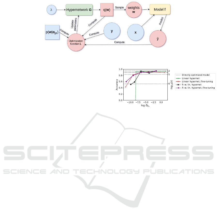
Figure 2: The diagram of the hypernetwork training. All the given variables are marked in blue. All the variables to optimize

are marked in red.

For all the experiments we considered model clas-

siﬁcation accuracy as a quality criterion. We used

ADAM optimizer with a learning rate 5 · 10

−4

. As

logarithm of the variance for the variational distribu-

tion at initialization α

we used −3.0; as the prior

variance we use α

= 1.0. For each of the models we

carried out 5 runs, the results were averaged.

4.1 Preserving of Statistical Properties

For the ﬁrst experiment, we used the Wine dataset,

consisting of 178 objects categorized into 3 classes.

Our main goal of this experiment was to demon-

strate that the hypernetworks can preserve the sta-

tistical properties of the approximated model. For

this experiment, we split the dataset into 142 objects

for the train and 36 objects for the test. We used

variational linear model (9) as a basic classiﬁcation

model optimized directly without hypernetwork. We

used two types of hypernetworks to approximate this

model: variational linear hypernetwork (12) and vari-

ational piecewise-linear hypernetwork (13) with N=5

piecewise-linear regions.

We used optimization with minibatch size set to

1. We trained every model for 200 epochs. We used

Λ =∈ [10

;10

]. This set was designed to consider

models with different performances: from slightly

regularized models with accuracy ≈ 95% to overreg-

ularized models with accuracy ≈ 53%.

Since our goal was not to obtain the highest accu-

racy using hypernetwork, but to obtain performance

and parameter distribution similar to the linear model,

we tracked the difference in the accuracy between

the hypernetwork and directly optimized model and

the difference between their distribution. For this

difference we used the symmetrized KL-divergence:

, q

) = D

, q

) + D

, q

), where q

is a variational distribution from hypernetwork, q

a variational distribution from the directly optimized

model. After the hypernetwork training, we also ﬁne-

tuned the obtained models for one epoch with ﬁxed

λ. We hypothesize that if the hypernetwork approx-

Figure 3: The results for the toy dataset for the directly opti-

mized model (9), linear hypernetwork (12) and piecewise-

linear hypernetwork (13) (P.-w. lin. hypernet). Each line

corresponds to the models performance obtained from hy-

pernetwork for different λ ∈ {10

, 10

imates the statistical properties of the directly opti-

mized model well, after ﬁne-tuning it will get accu-

racy closer to the directly optimized model, and its

will also decrease.

The results are shown in Figure 3. The gray

lines correspond to the accuracy values for different

λ ∈ {10

, 10

} obtained by directly op-

timized models. The x-axis corresponds to the loga-

rithm of

, therefore the perfect approximation of

the directly optimized model should be represented

by a line with points corresponding to the gray lines

on the y-axis and very low values on the x-axis. As

we can see, the linear hypernetwork poorly approxi-

mates the directly optimized model in comparison to a

more complex piecewise-linear hypernetwork that il-

lustrates the result of Theorem 2: the better model can

approximate the directly optimized model in terms

of optimization, the better it preserves its statisti-

cal properties. After ﬁne-tuning the piecewise-linear

hypernetwork also improved its performance every-

where except λ = 10

, where it got a better

result,

but worse accuracy. Note that training the model (9)

from scratch with only one epoch gave us accuracy

from 0 to 61% for different λ. This shows that the hy-

pernetworks really contained parameter distribution

close to the parameter distribution of the directly op-

timized model, the ﬁne-tuning step only increased its

performance, but not fully retrained the distribution

parameters. It also gives us a real scenario for the hy-

pernetwork usage: to store one set of parameters for

ICAART 2023 - 15th International Conference on Agents and Artiﬁcial Intelligence

models with different complexity to tune them to the

desired complexity on demand.

4.2 MNIST and CIFAR-10:

Experimental Settings

The main goals of these experiments is to demonstrate

the availability of the hypernetworks to generate the

deep learning model parameters with the condition on

the complexity value λ. As we obtain the parameters

for the desired model we prune it to check how many

informative ones have each of the models depending

on the complexity value λ. This experiment allows

us to compare properties of models which parameters

were obtained from hypernetwork with properties of

directly optimized ones.

For both the experiment we trained our models for

50 epochs. The minibatch size is set to 256. The fol-

lowing implementations were compared:

(a) variational neural network (9);

(b) network with covariance reparametrization (10);

(d) variational linear hypernetwork (12);

(e) network with covariance; reparametrization (10)

with linear hypernetwork (12);

(f) base network (11) (Lorraine and Duvenaud, 2018)

with linear hypernetwork (12);

(g) variational piecewise-linear hypernetwork (13),

N = 5;

(h) network with covariance reparametrization (10)

with piecewise-linear hypernetwork (13), N = 5;

(i) base network (11) (Lorraine and Duvenaud, 2018)

with piecewise-linear hypernetwork (13), N = 5.

We launched the neural network training for dif-

ferent values of the complexity value λ ∈ Λ. The pa-

rameters of each model were pruned after the opti-

mization using the g

var

criterion (17). For the imple-

mentations (c), (f), (i) we used the simpliﬁed criterion

simple

(18).

4.3 MNIST Experiment Results

For the MNIST dataset we used a neural network con-

sisting of two layers with 50 and 10 neurons, where

the second layer contains the softmax function. Pa-

rameters L, R for uniform distribution were set to −3

and 3 correspondingly.

Fig. 4a shows how the accuracy changes when

parameters were pruned for variational neural net-

work (9). The graph shows that the variational

method allows to remove ≈ 60% parameters for λ ∈

{10

−3

, 10

−2

, 10

−1

, 10

} and ≈ 80% parameters

for λ = 10

without signiﬁcant loss of classiﬁcation

accuracy. If we delete more parameters, the accuracy

for all values decreases. For large values of λ > 10

we obtain an oversimpliﬁed model. It contains a small

number of informative parameters. Thus, removing

of them for a given value of λ has little effect on the

classiﬁcation accuracy. However, the initial accuracy

is low.

Fig. 4d shows how the classiﬁcation accuracy

changes for the model with covariance reparametriza-

tion (10). Fig. 4g shows how the classiﬁcation accu-

racy changes for the base network (11). The classiﬁ-

cation accuracy of these two models hardly changed,

but the networks with the variational approach were

more robust to parameter deletion.

Fig. 4b, e, h shows how the classiﬁcation accuracy

changes when parameters are removed by the speci-

ﬁed method for models with the linear hypernetworks.

As can be seen from the graph, the average classi-

ﬁcation accuracy for all values of λ ∈ Λ, increased.

The deviation from the mean also increased for the

big percents of deleted parameters. At the same time,

for all values of λ ∈ Λ, a more stable models were

obtained: the classiﬁcation accuracy less depends on

the removal of parameters.

Fig. 4c, f, i shows how the classiﬁcation accuracy

changes when parameters were removed by the speci-

ﬁed method for a model with the piecewise-linear ap-

proximation. Models with the piecewise-linear hy-

pernetwork showed similar behaviour to models that

were trained directly during pruning. Moreover, for

all values of λ ∈ Λ, a more stable models were ob-

tained. All results are presented in the Table 1 and on

Fig. 5, where results for all λ were averaged.

4.4 CIFAR-10 Experiment Results

For the CIFAR-10 dataset, we used CNN-based archi-

tecture with convolutional layers of size (3,48), (48,

96), (96, 192), (192, 256), ReLU activation, and feed-

forward layer in the end. Parameters L, R for uniform

distribution were set to −2 and 0 correspondingly.

It can be seen from the Fig. 6a that the varia-

tional method also allowed removing ≈ 60% parame-

ters for λ = 0.01, 0.1, in contrast to the base model

Fig. 6d, where the classiﬁcation accuracy dropped

signiﬁcantly when 40 percent of the parameters were

removed.

The network with covariance reparametriza-

tion (10) showed poor results for CIFAR-10. They

are presented on the Fig. 8. The poor results can be

mainly explained by the specialty of (5) for the mod-

Deep Learning Model Selection With Parametric Complexity Control

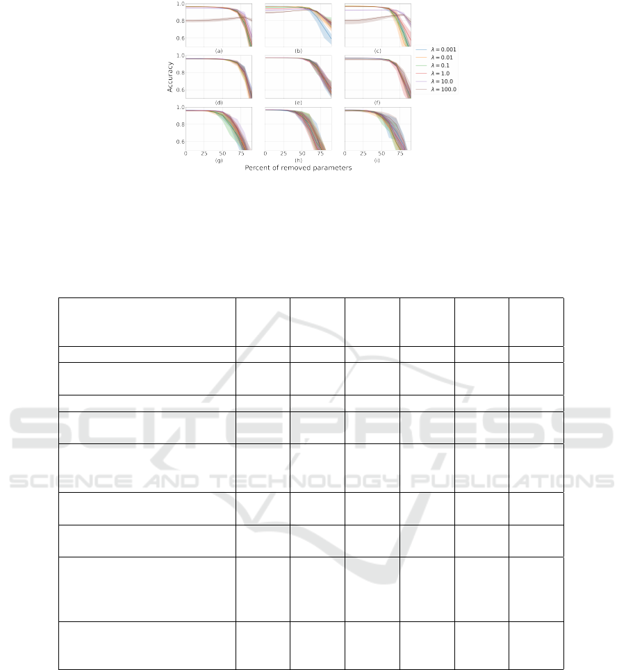
Figure 4: The dependence graph of the classiﬁcation accuracy on the percentage of removed parameters on MNIST dataset

for: (a) variational neural network (9), (b) variational linear hypernetwork (12), (c) variational piecewise-linear hypernet-

work (13); (d) network with covariance reparametrization (10), (e) network with covariance reparametrization (10) with

linear hypernetwork (12), (f) network with covariance reparametrization (10) with piecewise-linear hypernetwork (13); (g)

base network (11), (h) base network (11) with linear hypernetwork (12), (i) base network (11) with piecewise-linear hyper-

network (13).

Table 1: Accuracy after pruning for MNIST dataset.

Implemenatation/

Percent of deleted

parameters

0% 10% 30% 50% 70% 90%

Variational network 0.9676 0.9678 0.9661 0.9602 0.9350 0.8280

Network with covariance

reparametrization

0.9667 0.9668 0.9665 0.9605 0.9388 0.6208

Base net 0.9662 0.9659 0.9630 0.9563 0.8613 0.4917

Variational linear

hypernetwork

0.9703 0.9700 0.9699 0.9652 0.9182 0.8393

Network with

covariance reparametrization

with linear hypernetwork

0.9752 0.9749 0.9743 0.9698 0.9198 0.7039

Base network

with linear hypernetwork

0.9723 0.9719 0.9687 0.9527 0.8119 0.3470

Variational piecewise-linear

hypernetwork

0.9736 0.9733 0.9712 0.9621 0.9280 0.8229

Network with

covariance reparametrization

with piecewise-linear

hypernetwork

0.9706 0.9707 0.9701 0.9630 0.9186 0.6545

Base network

with piecewise-linear

hypernetwork

0.9710 0.9699 0.9656 0.9474 0.8774 0.3807

els with a large number of parameters, which is also

conﬁrmed by (8). We see that while the λ parameter

monotonously controls the inﬂuence of the prior dis-

tribution p(w|α

) in (4), there is no such monotonic-

ity for (5), therefore the calibration of the parameter

for the such a model is a more difﬁcult task and the

scale for the λ parameter can drastically differ for (5)

and (4),(6).

Fig. 6b, e shows graphs for variational (9) and

base (11) models with a linear hypernetwork (12).

As we can see, the classiﬁcation accuracy improved

for all λ ∈ Λ and the model’s robustness to parameter

deletion increased.

The same results(Fig. 6c,f) were reached with

piece-wise implementation of hypernetwork (13). In

addition, the piece-wise hypernetwork better approx-

imated the behaviour of directly trained models.

All the results for CIFAR-10 dataset are presented

in Table 2 and Fig. 7. The experiments show that

the variational (4) and the base (6) loss functions

give great and interpreted results. Despite the good

result on MNIST dataset, function with covariance

ICAART 2023 - 15th International Conference on Agents and Artiﬁcial Intelligence

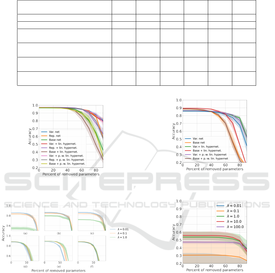
Table 2: Accuracy after pruning for CIFAR-10 dataset.

Implemenatation/

Percent of deleted parameters

0% 10% 30% 50% 70% 90%

Variational network 0.8612 0.8614 0.8615 0.8508 0.8048 0.4577

Base net 0.8852 0.8839 0.8728 0.8191 0.5683 0.1582

Variational linear

hypernetwork

0.8719 0.8719 0.8691 0.8520 0.8189 0.6107

Base network

with linear hypernetwork

0.8984 0.8984 0.8919 0.8683 0.7565 0.1656

Variational piecewise-linear

hypernetwork

0.8720 0.8715 0.8703 0.8561 0.8207 0.5173

Base network

with piecewise-linear hypernetwork

0.8879 0.8868 0.8752 0.8321 0.5146 0.1354

Figure 5: The dependence graph of the classiﬁcation accu-

racy on the percentage of removed parameters for all mod-

els on MNIST dataset.

Figure 6: The dependence graph of the classiﬁcation accu-

racy on the percentage of removed parameters on CIFAR-

10 dataset for: (a) variational neural network (9), (b) vari-

ational linear hypernetwork (12), (c) variational piecewise-

linear hypernetwork (13); (d) base network (11), (e) base

network (11) with linear hypernetwork (12), (f) base net-

work (11) with piecewise-linear hypernetwork (13).

reparametrization (5) requires more accurate tuning

for different models and data, that is why it is not

suitable in many cases. In addition, experiments show

that we can obtain a hypernetwork that precisely ap-

proximates original network. This result supports the

Theorem 2.

Figure 7: The dependence graph of the classiﬁcation accu-

racy on the percentage of removed parameters for all mod-

els on CIFAR-10 dataset.

Figure 8: The dependence graph of the classiﬁcation ac-

curacy on the percentage of removed parameters for net-

work with covariance reparametrization (10) on CIFAR-10

dataset.

5 CONCLUSION

This paper investigated the problem of deep learning

model complexity control at the inference. To control

the model complexity, we introduced probabilistic as-

sumptions about the distribution of parameters of the

deep learning model. The paper analyzed three forms

of regularization to control the model parameter dis-

Deep Learning Model Selection With Parametric Complexity Control

tribution. It generalized the model evidence as a crite-

rion that depends on the required model complexity.

The proposed method was based on the representa-

tion of deep learning model parameters in the form

of hypernetwork output. We analyzed this method in

the computational experiments on the Wine, MNIST

and CIFAR-10 datasets. The results showed that mod-

els with hypernetworks have the same properties as

models trained directly but use less computational re-

sources. Furthermore, these models are more sta-

ble in terms of deleting parameters and can be eas-

ily adjust to computational restrictions. In future, we

are going to research other variants of hypernetwork

implementation and advanced methods of controlling

model’s complexity. Besides, it is still a question how

to choose the complexity parameter λ for new dataset.

We plan to investigate it in future research.

REFERENCES

Atanov, A., Ashukha, A., Struminsky, K., Vetrov, D., and

Welling, M. (2019). The deep weight prior. In Inter-

national Conference on Learning Representations.

Bakhteev, O. and Strijov, V. (2018). Deep learning model

selection of suboptimal complexity. Automation and

Remote Control, 79:1474–1488.

Bishop, C. M. (2006). Pattern Recognition and Machine

Learning. Springer.

Blake, C. (1998). Uci repository of machine learn-

ing databases. http://www. ics. uci. edu/˜

mlearn/MLRepository. html.

Graves, A. (2011). Practical variational inference for neural

networks. In Shawe-Taylor, J., Zemel, R. S., Bartlett,

P. L., Pereira, F. C. N., and Weinberger, K. Q., editors,

Advances in Neural Information Processing Systems

24: 25th Annual Conference on Neural Information

Processing Systems 2011. Proceedings of a meeting

held 12-14 December 2011, Granada, Spain, pages

2348–2356.

Ha, D., Dai, A. M., and Le, Q. V. (2016). Hypernetworks.

CoRR, abs/1609.09106.

Han, S., Pool, J., Tran, J., and Dally, W. (2015). Learning

both weights and connections for efﬁcient neural net-

work. In Cortes, C., Lawrence, N., Lee, D., Sugiyama,

M., and Garnett, R., editors, Advances in Neural Infor-

mation Processing Systems, volume 28. Curran Asso-

ciates, Inc.

Jiang, T., Yang, X., Shi, Y., and Wang, H. (2019). Layer-

wise deep neural network pruning via iteratively

reweighted optimization. In ICASSP 2019 - 2019

IEEE International Conference on Acoustics, Speech

and Signal Processing (ICASSP), pages 5606–5610.

Krizhevsky, A., Nair, V., and Hinton, G. (-). Cifar-10 (cana-

dian institute for advanced research).

LeCun, Y. and Cortes, C. (2010). MNIST handwritten digit

database. http://yann.lecun.com/exdb/mnist/.

Lorraine, J. and Duvenaud, D. (2018). Stochastic hyperpa-

rameter optimization through hypernetworks. CoRR,

abs/1802.09419.

Louizos, C., Ullrich, K., and Welling, M. (2017). Bayesian

compression for deep learning. In Guyon, I., Luxburg,

U. V., Bengio, S., Wallach, H., Fergus, R., Vish-

wanathan, S., and Garnett, R., editors, Advances in

Neural Information Processing Systems, volume 30.

Curran Associates, Inc.

Zhmoginov, A., Sandler, M., and Vladymyrov, M. (2022).

Hypertransformer: Model generation for supervised

and semi-supervised few-shot learning. arXiv preprint

arXiv:2201.04182.

ICAART 2023 - 15th International Conference on Agents and Artiﬁcial Intelligence