Benchmarking Disease Modeling Techniques on the Philippines’

COVID-19 Dataset

Christian Pulmano

and Proceso Fernandez

Department of Information Systems and Computer Science, Ateneo de Manila University, Quezon City, Philippines

Keywords:

Mathematical Modeling, Parameter Estimation, ARIMA, COVID-19.

Abstract:

The COVID-19 pandemic has emphasized the importance of timely and accurate prediction of disease out-

breaks. Mathematical disease models can help simulate the trajectory of diseases and guide policymakers in

identifying priorities and gaps in current policies. This study evaluates the performance, on various metrics,

of three different parameter estimation algorithms in compartmental models, i.e., Nelder-Mead, Simulated

Annealing, and L-BFGS-B, together with the ARIMA time-series modeling, in modeling COVID-19 cases.

Using the daily number of conﬁrmed cases of COVID-19 in the Philippines as the dataset, the models were

trained on 90 different periods, with each period having 30 days of case data. After training, the models were

used to predict the cases up to 30 days later. The Negative Log Likelihood (NLL), time spent, iterations per

second, and memory allocation were all measured. The results show that ARIMA performed better in terms

of accuracy, time, and space efﬁciency than each of the other algorithms. This suggests that ARIMA should

be preferred for predicting the number of cases. However, policymaking sometimes requires scenario-based

modeling, which ARIMA is unable to provide. For such requirements, any of the three compartmental models

may be preferred, as each performed generally very well, too.

1 INTRODUCTION

Disease modeling has always been vital for health

planning and policymaking during disease outbreaks

and epidemics. In some areas, disease modeling

has been a standard practice for decision-making

(Kretzschmar, 2020) at the local and national levels

(de Lara-Tuprio et al., 2022). The COVID-19 pan-

demic recently emphasized further the need to pro-

duce accurate disease models as the world raced to

mitigate the spread of the disease.

Some standard methodologies used for disease

modeling are compartmental models using ordi-

nary differential equations and time-series modeling.

Mathematical models are often implemented when

studying the spread of diseases (Panovska-Grifﬁths,

2020). The increase in computing power has already

advanced the development of disease models. How-

ever, further optimizations can still be applied to gen-

erate more sophisticated models more efﬁciently.

One crucial step in compartmental disease mod-

eling is parameter estimation. When model parame-

ters are unknown and cannot be derived from existing

datasets and models, the values can be estimated us-

https://orcid.org/0000-0001-7870-8197

https://orcid.org/0000-0001-5370-4544

ing parameter estimation methodologies. This kind of

optimization problems is also relevant to other ﬁelds

aside from epidemiology, including ﬁnance, physics,

biology, and engineering (Rica and Ruz, 2020). Mod-

elers need to perform the parameter estimation pro-

cess on a regular basis (de Lara-Tuprio et al., 2022)

as new data are generated. In some cases, the param-

eter estimation problem can get computationally ex-

pensive, especially when the model designs become

complex (Akman et al., 2018).

Alternatively, time-series approaches such

as Auto-Regressive Integrated Moving Average

(ARIMA) can also be used to model the spread of

diseases (Tandon et al., 2020). During the COVID-19

pandemic, ARIMA models have been used to do

short-term predictions (Anne and Jeeva, 2020) on

the number of cases (Tandon et al., 2020). ARIMA

has been shown to provide valuable insights for

COVID-19 epidemiological surveillance efforts (Roy

et al., 2021).

This study evaluates the performance of differ-

ent parameter estimation algorithms, and the ARIMA

time-series modeling, in modeling the trend of

COVID-19 cases in the Philippines. The study aims to

create a benchmark that may provide insights toward

developing more efﬁcient disease models that can be

embedded into health decision support systems.

264

Pulmano, C. and Fernandez, P.

Benchmarking Disease Modeling Techniques on the Philippines’ COVID-19 Dataset.

DOI: 10.5220/0011626400003414

In Proceedings of the 16th International Joint Conference on Biomedical Engineering Systems and Technologies (BIOSTEC 2023) - Volume 5: HEALTHINF, pages 264-270

ISBN: 978-989-758-631-6; ISSN: 2184-4305

 2023 by SCITEPRESS – Science and Technology Publications, Lda. Under CC license (CC BY-NC-ND 4.0)

The paper is organized as follows: Section 2 pro-

vides a review of past researches and related works,

Section 3 outlines the methodology for the study, Sec-

tion 4 presents the results of the experiments, and Sec-

tion 5 summarizes the conclusions of the study.

2 REVIEW OF RELATED

LITERATURE

2.1 Mathematical Modeling and

Parameter Estimation

Mathematical models are commonly used to study the

dynamics and spread of diseases (Mohamadou et al.,

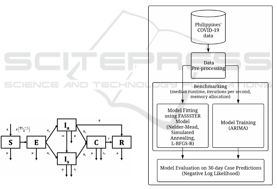
2020). In the Philippines, the FASSSTER compart-

mental model, whose visual representation is shown

in Figure 1, is used as a toolkit for modeling the

spread of COVID-19. The model is composed of

six compartments: Susceptible (S), Exposed (E), In-

fectious but asymptomatic (I

), Infectious but symp-

tomatic (I

), Conﬁrmed (C), and Recovered (R). The

transmissions between compartments are computed

using ordinary differential equations, where param-

eter values describe the rate of transmission from one

compartment to another. In the FASSSTER model,

some parameters were derived from existing data and

taken from literature, but some unknown parameters

and state values were estimated using parameter es-

timation by model ﬁtting. The results of the model

have contributed signiﬁcantly to the policymaking ef-

forts of the Philippines’ national government through-

out the pandemic (de Lara-Tuprio et al., 2022).

Figure 1: FASSSTER COVID-19 compartmental model.

2.2 Time-Series Modeling

Statistical methods such as time-series models have

also been applied in disease forecasting and predic-

tion. Studies in the past have used time-series mod-

els in estimating incidence and prevalence of dis-

eases like inﬂuenza, malaria, and COVID-19 (Cey-

lan, 2020). One study used ARIMA to predict the

number of deaths related to COVID-19. In said study,

ARIMA was able to forecast the possible number of

deaths where the average absolute percentage error

validated the model by 99.09% (Chaurasia and Pal,

2020) indicating a good performance of the model.

As shown in past studies, both methods pro-

vide reliable solutions for disease modeling prob-

lems. However, they also have their own strengths

and weaknesses. As such, the remaining sections of

this paper describe an evaluation of the performance

of these methods when used in a disease modeling

problem.

3 METHODOLOGY

The methodology of the study is illustrated in Figure

Figure 2: Methodology of the study.

3.1 Dataset and Pre-Processing

The Philippines’ COVID-19 dataset was extracted as

a CSV ﬁle from the Department of Health - Philip-

pines (DOH Philippines) COVID-19 tracker (Depart-

ment of Health, 2020). The initial dataset consisted

of anonymized individual case data from March 2020

Benchmarking Disease Modeling Techniques on the Philippines’ COVID-19 Dataset

265

to September 2022. However, the study only focused

on data from April 2020 to July 2020 since this was

when the identiﬁed version of the FASSSTER model

was heavily adopted, and thus the model parameter

values are more appropriate. The individual case data

were aggregated to get the daily number of new cases

in the Philippines. Although the FASSSTER model

was also used for modeling COVID-19 for smaller

administrative areas, this study only focused on the

national level. The national daily case data was used

for the model ﬁtting/training and evaluation.

3.2 Model Development and Simulation

The objective of the study is to evaluate various pa-

rameter estimation algorithms in a compartmental

disease model, and the ARIMA time-series model.

Both the compartmental and ARIMA time-series

models were developed using the R programming lan-

guage.

The FASSSTER model was adopted for the

COVID-19 compartmental model. The initial con-

ditions, known parameters, and parameters to be es-

timated were also based from the FASSSTER study

(de Lara-Tuprio et al., 2022). Three parameter esti-

mation algorithms, i.e., Nelder-Mead, Simulated An-

nealing, and L-BFGS-B, were evaluated for the com-

partmental model. The models were ﬁtted to the ac-

tual case data based on the minimum negative log

likelihood (NLL) using Poisson distribution.

Both the compartmental disease models and

ARIMA time-series models were ﬁtted/trained using

training data consisting of 30 days of daily COVID-

19 case counts starting from April 1 2020 to June 30

2020, totalling to 91 time periods. The resulting mod-

els were then used to predict the cases up to 30 days

forward.

3.3 Model Evaluation

The bench package of R was used to measure the me-

dian run time in seconds, total memory allocation in

megabytes (MB), and iterations per second on 5 it-

erations during the model ﬁtting/training. The 30-

day model predictions were then compared with ac-

tual case data as reported by DOH Philippines. The

NLL was computed to measure the accuracy of the

case predictions.

One-way Analysis of Variance (ANOVA) was

used to test if there are statistical differences among

the model outputs. Further, the Tukey Honest Signiﬁ-

cance Difference (Tukey HSD) test was implemented

to determine which speciﬁc pairs of modeling tech-

niques have signiﬁcant differences. Tukey HSD in-

corporates some corrections, with such corrections

becoming necessary when multiple pairs are tested

for differences. An alternative correction is used in

the Bonferroni test, which is probably the simplest

among post hoc tests, and is conservative on Type I

errors but is however more prone to Type II errors.

4 RESULTS AND DISCUSSIONS

4.1 Negative Log Likelihood

Table 1 summarizes the NLL values based on the 30-

day predictions of new cases using the different dis-

ease modeling methods. The ARIMA model had the

lowest mean NLL value at 13074.85 and the lowest

median value at 9178.40. Although the overall mini-

mum NLL value was produced using Simulated An-

nealing at 1070.86, the minimum NLL for ARIMA,

1104.75, is only at a slight difference. ARIMA

also had the lowest standard deviation with a value

of 13442.28, signifying that the NLL values com-

puted from the ARIMA model predictions are closer

to the mean value. Among the group, L-BFGS-B

had the highest mean NLL value of 438883.18, fol-

lowed by Nelder-Mead, with a mean NLL value of

39248.45. Nelder-Mead produced the overall maxi-

mum NLL value of 1041587.03 and the highest NLL

standard deviation at 112435.38. L-BFGS-B and

Nelder-Mead also provided the highest median NLL

values at 13434.54 and 13432.61, respectively.

Table 1: Summary of negative log likelihood values for each

method.

method mean median min max stdev

NM 39248.45 13432.61 3477.48 1041587.03 112435.38

SANN 27801.88 11956.06 1070.86 454141.05 57790.56

L-BFGS-B 43883.18 13434.54 2976.53 391733.97 77462.12

ARIMA 13074.85 9178.40 1104.75 81025.72 13442.28

A box plot representation of the NLL values in

logarithmic scale for each method is shown in Figure

3. The resulting NLL values suggest that the case pre-

dictions using Nelder-Mead and L-BFGS-B have the

least likelihood. ARIMA mostly provided the best

NLL values, which suggests that ARIMA should be

preferred to predict new cases with the most likeli-

hood. However, it might still be worth investigat-

ing if the parameters, initial conditions, and hyper-

parameters that were used for the parameter estima-

tion algorithms are approximately optimal.

A one-way ANOVA was performed to compare

the NLL values of the four disease-modeling meth-

ods. The one-way ANOVA revealed that there was

a signiﬁcant difference in the mean NLL scores be-

HEALTHINF 2023 - 16th International Conference on Health Informatics

266

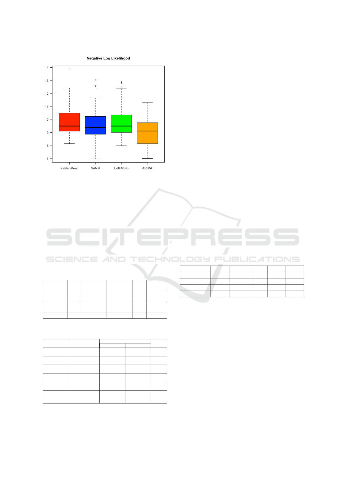
Figure 3: Box plot representation of NLL values for each

method in logarithmic scale.

tween at least two groups (p = 0.0298). The sum-

mary is shown in Table 2. Tukey HSD Test for

pairwise comparisons found the mean NLL value

was signiﬁcantly different between L-BFGS-B and

ARIMA (p=0.034), and no signiﬁcant differences in

the mean NLL scores of Nelder-Mead and ARIMA

(p=0.084), SANN-ARIMA (p=0.541), Nelder-Mead

and L-BFGS-B (p=0.977), SANN and L-BFGS-B

(p=0.485), and SANN and Nelder-Mead (p=0.727).

The summary of the results of Tukey HSD is shown

in Table 3.

Table 2: Results of one-way ANOVA on NLL values.

df Sum of

Squares

Mean

Square

F p-value

Between

Groups

3 5.011E+10 1.670E+10 3.02 0.0298

Within

Groups

352 1.947E+12 5.530E+09

Total 355 1.997E+12

Table 3: Pairwise tests using Tukey HSD on NLL values.

Mean Difference 95% Conﬁdence Interval p-value

Lower Bound Upper Bound

L-BFGS-B

-ARIMA

30808.332 1672.273 59944.390 0.034

Nelder-Mead

-ARIMA

26173.600 -2284.784 54631.980 0.084

SANN

-ARIMA

14727.030 -13731.354 43185.410 0.541

Nelder-Mead

-L-BFGS-B

-4634.733 -33770.792 24501.330 0.977

SANN

-L-BFGS-B

-16081.303 -45217.362 13054.760 0.485

SANN

-Nelder-

Mead

-11446.570 -39904.954 17011.810 0.727

4.2 Median Run Time and Iterations

per Second

The median run time (measured in seconds) and it-

erations per second measure the latency and through-

put of model training, respectively. The results were

aligned with the expectation that ARIMA will per-

form better than the other techniques due to its sim-

pler model design as compared to the other disease

modeling techniques. The summary values are shown

in Tables 4 and 7.

In terms of median run time, ARIMA was the

fastest having a mean value of 0.02 seconds, median

value of 0.02 seconds, and overall minimum value of

0.01 seconds. The maximum value of ARIMA at 0.07

seconds was also faster than the minimum values of

the other methods. Between Nelder-Mead and Simu-

lated Annealing, Nelder-Mead was consistently faster

having a mean value of 2.38 seconds, median value

of 2.27 seconds, and minimum value of 1.31 seconds.

Simulated Annealing provided a mean value of 2.93

seconds, median value of 2.81 seconds and minimum

value of 2.07 seconds. L-BFGS-B was the slowest

among the group having a mean value of 16.83 sec-

onds, median value of 9.20 seconds, minimum value

of 2.94 seconds, and reaching a maximum value of

66.84 seconds. Figure 4 shows a box plot representa-

tion of the median runtime values for each method.

Table 4: Summary of median run time values for each

method.

method mean median min max stdev

NM 2.38 2.27 1.31 3.99 0.63

SANN 2.93 2.81 2.07 4.87 0.62

L-BFGS-B 16.83 9.20 2.94 66.84 16.76

ARIMA 0.02 0.02 0.01 0.07 0.01

The one-way ANOVA result, as shown in Table 5,

reveals that there is a signiﬁcant difference between at

least two groups (p<2E-16). Tukey HSD test further

shows that there are signiﬁcant differences between

L-BFGS-B and ARIMA (p=0), Nelder-Mead and L-

BFGS-B (p=0), and SAAN and L-BFGS-B (p=0). It

is revealed however that there are no signiﬁcant differ-

ence between Nelder-Mead and ARIMA (p=0.203),

SANN and ARIMA (p=0.075), and between SANN

and Nelder-Mead (p=0.969). The summary of Tukey

HSD is displayed in Table 6.

In terms of iterations per second, only ARIMA

performed multiple iterations of the model training in

a second. ARIMA provided a mean value of 49 iter-

ations, a median of 46 iterations, minimum of 14 it-

erations, and a maximum of 114 iterations. The other

methods all resulted in having less than one iteration

Benchmarking Disease Modeling Techniques on the Philippines’ COVID-19 Dataset

267

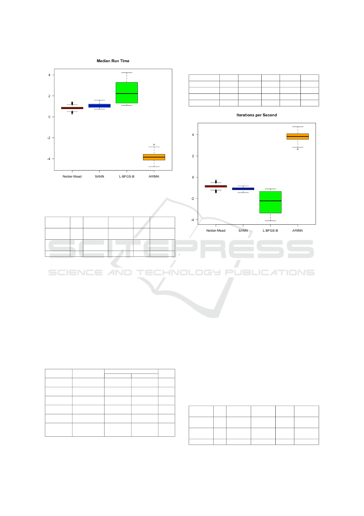
Figure 4: Box plot representation of median run time (sec-

onds) values for each method in logarithmic scale.

Table 5: Results of one-way ANOVA on median runtime

values.

df Sum of

Squares

Mean

Square

F p-value

Between

Groups

3 14848 4949 75.44 <2E-16

Within

Groups

352 23094 66

Total 355 37942

per second. The values are represented in Figure 5.

The results of one-way ANOVA for iterations

per second values reveal that there is a signiﬁcant

difference between at least two groups (p<2E-16).

The Tukey HSD test shows that there are signiﬁ-

cant differences in the mean iterations per second val-

ues between L-BFGS-B and ARIMA (p=0), Nelder-

Mead and ARIMA (p=0), SANN and ARIMA (p=0),

but no signiﬁcant difference between Nelder-Mead

and L-BFGS-B (p=0.998), SANN and L-BFGS-B

(p=0.999), and between SANN and Nelder-Mead

(p=1.000).

Table 6: Pairwise tests using Tukey HSD on median runtime

values.

Mean Difference 95% Conﬁdence Interval p-value

Lower Bound Upper Bound

L-BFGS-B

-ARIMA

16.804 13.631 19.978 0.000

Nelder-Mead

-ARIMA

2.361 -0.739 5.460 0.203

SANN

-ARIMA

2.907 -0.193 6.006 0.075

Nelder-Mead

-L-BFGS-B

-14.444 -17.617 -11.270 0.000

SANN

-L-BFGS-B

-13.898 -17.071 -10.724 0.000

SANN

-Nelder-

Mead

0.546 -2.554 3.646 0.969

Table 7: Summary of iterations per second values for each

method.

method mean median min max stdev

NM 0.44 0.43 0.23 0.75 0.11

SANN 0.33 0.33 0.23 0.44 0.05

L-BFGS-B 0.14 0.11 0.02 0.33 0.10

ARIMA 49.53 46.14 14.00 114.50 21.53

Figure 5: Box plot representation of iteration per second

values for each method in logarithmic scale.

4.3 Memory Allocation

Table 10 summarizes the total memory allocations

during the model training. Similar to the median run

time and iterations per second, it was expected that

ARIMA will also perform better in terms of mem-

ory allocation. The results show that ARIMA consis-

tently provided the lowest memory allocations having

a mean value of 3.05MB, median value of 2.74MB,

and overall minimum value of 0.58MB. This signi-

ﬁes that ARIMA was the most space efﬁcient method

among the group. Nelder-Mead was considered the

second most space efﬁcient method among the group

having a mean value 92.29MB, median value of

87.43MB, and minimum value of 51.18MB. Simu-

lated Annealing was the third most efﬁcient among

the group having a mean value of 120.01MB, median

value of 100.27MB, and minimum value of 84.77. L-

Table 8: Results of one-way ANOVA on iterations per sec-

ond values.

df Sum of

Squares

Mean

Square

F p-value

Between

Groups

3 164094 54698 461.60 <2E-16

Within

Groups

352 41710 118

Total 355 205804

HEALTHINF 2023 - 16th International Conference on Health Informatics

268

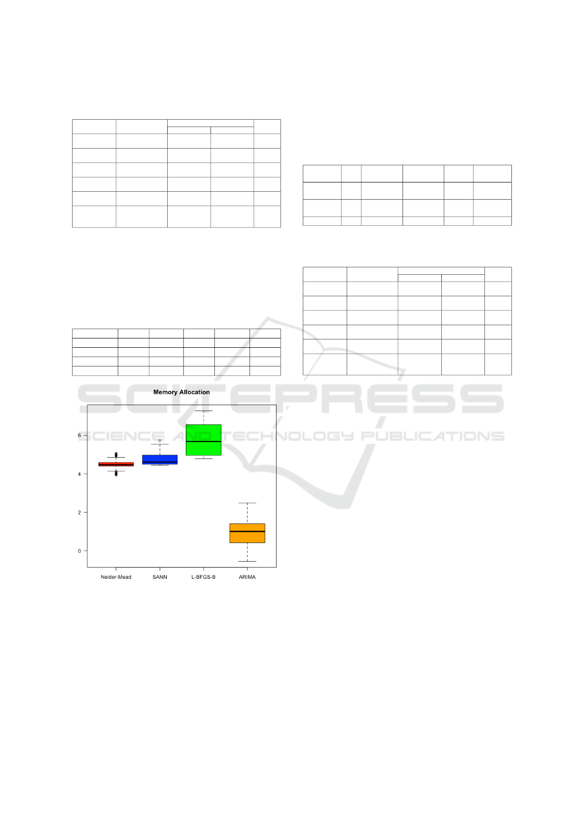
Table 9: Pairwise tests using Tukey HSD on iterations per

second values.

Mean Difference 95% Conﬁdence Interval p-value

Lower Bound Upper Bound

L-BFGS-B

-ARIMA

-49.386 -53.650 -45.121 0.000

Nelder-Mead

-ARIMA

-49.090 -53.256 -44.924 0.000

SANN

-ARIMA

-49.193 -53.359 -45.027 0.000

Nelder-Mead

-L-BFGS-B

0.296 -3.969 4.560 0.998

SANN

-L-BFGS-B

0.193 -4.072 4.458 0.999

SANN

-Nelder-

Mead

-0.103 -4.269 4.063 1.000

BFGS-B was least efﬁcient in terms of memory allo-

cations, having a mean value of 436.08MB, a median

value of 292.22MB, and overall maximum value of

1434.58MB. A box plot representation of memory al-

location values is shown in Figure 6.

Table 10: Summary of memory allocations for each

method.

method mean median min max stdev

NM 92.29 87.43 51.18 158.42 25.70

SANN 120.01 100.27 84.77 306.81 41.64

L-BFGS-B 436.08 292.22 119.98 1434.58 342.90

ARIMA 3.05 2.74 0.58 12.08 1.90

Figure 6: Box plot representation of memory allocation val-

ues for each method in logarithmic scale.

Table 11 shows the summary of one-way ANOVA

on memory allocation values. The results revealed

that there was a signiﬁcant difference in the mean

memory allocation values between at least two groups

(p<2E-16). Tukey HSD test further reveals the mean

memory allocation value was signiﬁcantly different

between L-BFGS-B and ARIMA (p=0), Nelder-Mead

and ARIMA (p=0.002), SANN and ARIMA (p=0),

Nelder-Mead and L-BFGS-B (p=0), and SANN and

L-BFGS-B (p=0), but no signiﬁcant difference be-

tween SANN and Nelder-Mead (p=0.679).

Table 11: Results of one-way ANOVA on memory alloca-

tion values.

df Sum of

Squares

Mean

Square

F p-value

Between

Groups

3 9.127E-06 3.042E-06 108.60 <2E-16

Within

Groups

352 9.858E-06 2.800E-08

Total 355 1.899E-05

Table 12: Pairwise tests using Tukey HSD on memory allo-

cation values.

Mean Difference 95% Conﬁdence Interval p-value

Lower Bound Upper Bound

L-BFGS-B

-ARIMA

4.3303E-04 3.6746E-04 4.9859E-04 0.000

Nelder-Mead

-ARIMA

8.9237E-05 2.5196E-05 1.5328E-04 0.002

SANN

-ARIMA

1.1696E-04 5.2920E-05 1.8100E-04 0.000

Nelder-Mead

-L-BFGS-B

-3.4379E-04 -4.0936E-04 -2.7822E-04 0.000

SANN

-L-BFGS-B

-3.1607E-04 -3.8163E-04 -2.5050E-04 0.000

SANN

-Nelder-

Mead

2.7724E-05 -3.6317E-05 9.1765E-05 0.679

5 CONCLUSIONS AND FUTURE

WORK

This study evaluates the performance of parameter es-

timation algorithms, and the ARIMA time-series in

model training and evaluation for COVID-19 disease

modeling using the Philippines’ COVID-19 dataset.

After measuring the performance of the different

methods on various metrics, the results show the

ARIMA has the best performance in terms of max-

imizing the likelihood of predictions, latency and

throughput of model training, and memory efﬁciency.

This may suggest that ARIMA is efﬁcient in the goal

of predicting the trends of the COVID-19 disease.

However, a limitation of ARIMA is scenario-based

modeling. Although the simulations show that the

parameter estimation algorithms weren’t as efﬁcient

as ARIMA, they are capable of accepting varying pa-

rameter values and modeling different scenarios of the

disease.

This work provides a groundwork for the develop-

ment of more efﬁcient algorithms for disease model-

ing. Future work will incorporate the results of this

study in order to develop more optimal algorithms

that can be used for epidemic planning and decision-

making. Ideally, efﬁcient disease models will be in-

corporated into health information systems such as

Benchmarking Disease Modeling Techniques on the Philippines’ COVID-19 Dataset

269

clinic management systems, pharmacy information

systems, and laboratory information systems to assist

health decisions-makers in their day-to-day decision-

making. The evaluations can also be done on data sets

other than the Philippines. Since disease modeling is

also a global need, it is also worth identifying how

the methodology and the outputs of this study can be

applied to a global environment.

ACKNOWLEDGEMENTS

The authors would like to acknowledge the Depart-

ment of Information Systems and Computer Science,

Ateneo de Manila University for their support to the

study.

REFERENCES

Akman, D., Akman, O., and Schaefer, E. (2018). Parameter

estimation in ordinary differential equations modeling

via particle swarm optimization. Journal of Applied

Mathematics, 2018.

Anne, W. R. and Jeeva, S. C. (2020). Arima modelling of

predicting covid-19 infections. medRxiv.

Ceylan, Z. (2020). Estimation of covid-19 prevalence in

italy, spain, and france. Science of The Total Environ-

ment, 729:138817.

Chaurasia, V. and Pal, S. (2020). Covid-19 pandemic:

Arima and regression model-based worldwide death

cases predictions. SN Computer Science, 1(5):1–12.

de Lara-Tuprio, E., Estadilla, C. D. S., Macalalag, J. M. R.,

Teng, T. R., Uyheng, J., Espina, K. E., Pulmano,

C. E., Estuar, M. R. J. E., and Sarmiento, R. F. R.

(2022). Policy-driven mathematical modeling for

covid-19 pandemic response in the philippines. Epi-

demics, 40:100599.

Department of Health (2020). Covid-19 tracker.

https://doh.gov.ph/covid19tracker.

Kretzschmar, M. (2020). Disease modeling for public

health: added value, challenges, and institutional con-

straints. Journal of public health policy, 41(1):39–51.

Mohamadou, Y., Halidou, A., and Kapen, P. T. (2020). A re-

view of mathematical modeling, artiﬁcial intelligence

and datasets used in the study, prediction and manage-

ment of covid-19. Applied Intelligence, 50(11):3913–

3925.

Panovska-Grifﬁths, J. (2020). Can mathematical modelling

solve the current covid-19 crisis?

Rica, S. and Ruz, G. A. (2020). Estimating sir model param-

eters from data using differential evolution: an appli-

cation with covid-19 data. In 2020 IEEE Conference

on Computational Intelligence in Bioinformatics and

Computational Biology (CIBCB), pages 1–6.

Roy, S., Bhunia, G. S., and Shit, P. K. (2021). Spatial pre-

diction of covid-19 epidemic using arima techniques

in india. Modeling earth systems and environment,

7(2):1385–1391.

Tandon, H., Ranjan, P., Chakraborty, T., and Suhag, V.

(2020). Coronavirus (covid-19): Arima based time-

series analysis to forecast near future. arXiv preprint

arXiv:2004.07859.

HEALTHINF 2023 - 16th International Conference on Health Informatics

270