Revisiting the DFT Test in the NIST SP 800-22 Randomness Test Suite

Hiroki Okada

and Kazuhide Fukushima

KDDI Research, Inc., Fujimino-shi, 356-8502 Japan

Keywords:

Randomness, RNG, NIST SP 800-22, Discrete Fourier Transformation.

Abstract:

The National Institute of Standards and Technology (NIST) released SP 800-22, which is a test suite for

evaluating pseudorandom number generators for cryptographic applications. The discrete Fourier transform

(DFT) test, which is one of the tests in NIST SP 800-22, was constructed to detect some periodic features of

input sequences. There was a crucial problem in the construction of the DFT test: its reference distribution

of the test statistic was not derived mathematically; instead, it was numerically estimated. Thus, the DFT

test was constructed under the assumption that the pseudorandom number generator (PRNG) used for the

estimation generated “truly” random numbers, which is a circular reasoning. Recently, Iwasaki (Iwasaki,

2020) performed a novel analysis to theoretically derive the correct reference distribution (without numerical

estimation). However, Iwasaki’s analysis relied on some heuristic assumptions.

In this paper, we present theoretical evidence for one of the assumptions. Let x

,··· ,x

n−1

be an n-bit input

sequence. Its Fourier coefﬁcients are deﬁned as F

,...,F

n−1

. Iwasaki assumed that

∑

−1

j=0

= n

/2. We

use a quantitative analysis to show that this holds when n is sufﬁciently large. We also verify that our analysis

is sufﬁciently accurate with numerical experiments.

1 INTRODUCTION

Random numbers are used in many applications, such

as cryptography and numerical simulations. However,

it is not easy to generate “truly” random sequences.

Pseudorandom number generators (PRNGs) generate

sequences by iterating a recurrence relation; there-

fore, the sequences are produced deterministically

and are not “truly” random. The binary “truly” ran-

dom sequence is deﬁned as the sequence of random

variables that have a probability of exactly

of being

“0” or “1” and are mutually independent: We can

write an n-bit “truly” random sequence as ε

,.. .,ε

iid

∼

U({0,1}).

NIST SP 800-22 (Rukhin et al., 2010; Bassham III

et al., 2010) is a well-known statistical test suite

for evaluating pseudorandom number generators for

cryptographic applications. This test suite consists of

15 tests, and every test is a hypothesis test, where the

hypothesis is that the input sequence is truly random.

If this hypothesis is not rejected in any of the tests, it

is concluded that the input sequences are random.

The discrete Fourier transform (DFT) test in NIST

SP 800-22 is of interest to us. This test was con-

structed to detect periodic features in an input se-

https://orcid.org/0000-0002-5687-620X

quence. It performs discrete Fourier transformation

on input sequences and constructs the test statistic

from the Fourier coefﬁcients.

Kim et al. (Kim et al., 2003; Kim et al., 2004)

reported that the DFT test in the original NIST SP

800-22 (Rukhin et al., 2010) has a crucial theoretical

problem. They reported that the reference distribution

of the test statistic of the DFT test was erroneously de-

rived. Kim et al. numerically estimated the distribu-

tion of the test statistic with sequences generated with

a more accurate PRNG and proposed a new DFT test

with an estimated distribution. Hamano (Hamano,

2005) also performed an analysis on the distribution

of the Fourier coefﬁcients in the original DFT test

and made the DFT test problems clearer; however,

the theoretical distribution of the test statistic was

not derived. In 2005, in response to these reports,

NIST revised the DFT test according to the report of

Kim et al. and published NIST SP 800-22 version

1.7. The DFT test has not been subsequently revised.

Pareschi et al. (Pareschi et al., 2012) reviewed the

DFT test included in NIST SP 800-22 version 1.7, and

they reported a more accurate numerical estimation

on the reference distribution of the DFT test than

that given by Kim et al. (Kim et al., 2003; Kim

et al., 2004). Okada and Umeno (Okada and Umeno,

2017) proposed another test based on discrete Fourier

366

Okada, H. and Fukushima, K.

Revisiting the DFT Test in the NIST SP 800-22 Randomness Test Suite.

DOI: 10.5220/0011626300003405

In Proceedings of the 9th International Conference on Information Systems Security and Privacy (ICISSP 2023), pages 366-372

ISBN: 978-989-758-624-8; ISSN: 2184-4356

 2023 by SCITEPRESS – Science and Technology Publications, Lda. Under CC license (CC BY-NC-ND 4.0)

transformation that can avoid the problem, but they

failed to theoretically derive the reference distribution

of the original test statistic.

Iwasaki (Iwasaki, 2020) ﬁnally solved this long-

standing open problem of the DFT test with a novel

analysis on the joint probability density function of

the (square of the absolute value of) Fourier coefﬁ-

cients. However, Iwasaki’s analysis relied on some

heuristic assumptions.

In the following subsections, we describe the de-

tails of the procedure of the DFT test (Sect. 1.1) and

the problem of the DFT test (Sect. 1.2).

Then, we clarify our contribution in Sect. 1.3.

1.1 The DFT Test

We describe the details of the procedure of the origi-

nal DFT test (DFTT

original

) from 2001 (Rukhin et al.,

2010), which was released before the revision in 2005

(Bassham III et al., 2010). The focus of this test is

the peak heights in the discrete Fourier transformation

of the input sequence. The purpose of this test is to

check whether the input sequence periodic features

indicate a deviation from the assumption of random-

ness.

1. Throughout this paper, let n be an even inte-

ger. The input sequence is an n-bit sequence

,··· , ε

n−1

∈ {0,1}. The null hypothesis of this

test is that

,··· , ε

n−1

iid

∼ U({0, 1}). (1)

2. Convert the input sequence to x

,··· , x

n−1

, where

= 2ε

−1 (i ∈{0,. .., n −1}).

3. Apply a discrete Fourier transform (DFT)

to x

,··· , x

n−1

to produce Fourier coefﬁcients

}

n−1

j=0

. The Fourier coefﬁcient F

and its real

and imaginary parts c

(X) and s

(X), respectively,

are deﬁned as follows:

n−1

∑

k=0

exp



2πk j



. (2)

4. Compute {|F

−1

j=0

. Note that {|F

n−1

are not

of concern because |F

| = |F

n−j

| holds.

5. Set a threshold value T

0.95

√

3n such that 95%

of {|F

−1

j=0

are < T

0.95

, assuming that Eq. (1)

holds.

According to NIST SP800-22,

is consid-

ered to follow χ

, and T

0.95

is deﬁned by the

following equation.

P(|F

| < T

0.95

) = P



0.95



0.95

−

dy = 1 −e

−

0.95

:= 0.95

∴ T

0.95

−nln(0.05) ≃

√

As several researchers (Kim et al., 2004; Hamano,

2005) reported, it is obvious that T

0.95

should be

set as T

0.95

−nln(0.05) without approxima-

tion (T

0.95

√

3n). Thus, T

0.95

−nln(0.05)

in the revised version of the DFT test (Bassham III

et al., 2010).

6. Count

= #



| < T

0.95

,0 ≤ j ≤

−1

If {|F

−1

j=0

are mutually independent, then under

the assumption of Eq. (1), N

can be considered

to follow B(

,0.95), where B is the binomial

distribution.

Since B(n, p) can be approximated as the normal

distribution N (np, np(1 − p)) when n is sufﬁ-

ciently large, we can approximate

∼ N



0.95

,(0.95)(0.05)



under the assumption of Eq. (1).

7. Compute a test statistic

d =

−0.95

(0.95)(0.05)

The test statistic d follows N (0,1) when n is

sufﬁciently large, under the assumption of Eq. (1).

8. Compute the P-value; p = erfc



|d|

√



If p < α, where α is the signiﬁcance level of the

DFT test, then it is concluded that the sequence

is not random. NIST recommends α = 0.01

(Bassham III et al., 2010). If p ≥α, conclude that

the sequence is random.

Perform steps 1 to 7 for m sample sequences and

compute m P-values {p

, p

,.. ., p

}. Then, we per-

form second-level tests I and II to test the proportion

of sequences passing the tests and the uniformity of

the distribution of the P-values {p

, p

,.. ., p

}. See

(Bassham III et al., 2010) for the details.

Revisiting the DFT Test in the NIST SP 800-22 Randomness Test Suite

367

1.2 The Problem of the DFT Test

Kim et al. (Kim et al., 2004) and Hamano (Hamano,

2005) reported that

does not follow N



0.95

,(0.95)(0.05)



and as a consequence, the test statistic d :=

−0.95

√

(0.95)(0.05)

does not follow N (0,1). Furthermore,

Kim et al. estimated that

∼ N



0.95

,(0.95)(0.05)



(3)

and d :=

−0.95

√

(0.95)(0.05)

∼N (0,1) using a secure hash

generator (G-SHA1) (Bassham III et al., 2010) as

a PRNG. According to this result, DFTT

original

was

revised in (Bassham III et al., 2010). The present DFT

test, denoted as DFTT

present

, has not been revised.

Furthermore, Pareschi et al. reported that the

numerical estimation is not sufﬁciently accurate; they

numerically estimated that

∼ N



0.95

,(0.95)(0.05)

3.8



, (4)

and d :=

−0.95

√

(0.95)(0.05)

3.8

∼ N (0,1). DFTT

present

and

DFTT

pareschi

are constructed based on numerical es-

timation using PRNGs. However, the randomness of

PRNGs are the target that should be evaluated with

a randomness test. Thus, these tests cannot be used

unless the reference distribution is mathematically

derived.

The crucial problem here is that the reference

distribution of N

(or the test statistic d), Eqs. (3)

and (4), are derived by the numerical estimation with

some PRNG. The DFT test is constructed under the

assumption that the PRNG that is used for the es-

timation generates truly random numbers, which is

circular reasoning.

Iwasaki (Iwasaki, 2020) ﬁnally solved this prob-

lem. He derived the reference distribution of N

(and d) theoretically (without the numerical estima-

tion with some PRNG), which is given as follows

∼ N



0.95

,(0.95)(0.05)

3.79



and d :=

−0.95

√

(0.95)(0.05)

3.79

∼ N (0, 1). This was re-

alized by a novel analysis of the joint probability

density function of the |F

|s.

However, the analysis by (Iwasaki, 2020) was

based on several heuristic assumptions:

• Assumption 1: The value of V(N

) can be an-

alyzed in a sufﬁciently correct manner even if

we consider

∼ χ

(χ-squared distribution

with 2 degrees of freedom, see Deﬁnition 2.2) for

sufﬁciently large n.

Note that

∼ χ

correctly.

• Assumption 2:

∑

−1

j=0

= n

/2 holds.

Note that by Parseval’s theorem (see Lemma 2.6),

∑

−1

j=0

+ |F

−|F

), correctly.

• Assumption 3 (Iwasaki, 2020, Assumption 3.1):

Let y := (|F

,.. .,|F

−1|

); then, y uniformly

distributes over the set

{y ∈ R

−1

| y

≥ 0, |y|

= n

/2}.

This assumption is used on the premise that As-

sumption 2 holds.

1.3 Our Contribution

In this paper, we show that Assumption 2 above holds

when n is sufﬁciently large. We rephrase Assumption

2 as follows

• Assumption 2’: lim

n→∞

∑

−1

j=0

−

= 0,

and we give the rigorous proof of Assumption 2’.

As previously mentioned, we have

−1

∑

j=0

+ |F

−|F

), (5)

by Parseval’s theorem. We analyze the distribution

of the term z :=

(|F

− |F

) and show that it

follows N (0,4) when n is sufﬁciently large. Specif-

ically, we analyze the characteristic function of z,

denoted by φ

(t), which satisﬁes that lim

n→∞

(t) =

exp(−8t

) and coincides with the characteristic func-

tion of N (0, 4). Furthermore, we perform an experi-

ment and conﬁrm that the empirical distribution of z

is close to N (0,4).

By the deﬁnition of z, we can rewrite Eq. (5) as

−1

∑

j=0

(1 +

·z).

As we prove that z ∼ N (0,4), we have z = O(1)

with overwhelming probability. Thus, we have

∑

−1

j=0

(1 + O(

)), and we conclude that

lim

n→∞

∑

−1

j=0

−

= 0, which proves Assump-

tion 2’.

2 PRELIMINARIES

Vectors are in column form and are written using bold

lowercase letters, e.g., x. The i-th component of x will

be denoted by x

. For any s ∈ N, the set of the ﬁrst s

nonnegative integers is denoted [s] = {0, 1,.. .,s −1}.

For any set X, U(X) denotes the uniform distri-

bution over the set X. For a random variable (or

ICISSP 2023 - 9th International Conference on Information Systems Security and Privacy

368

distribution) X, we denote the probability density

function (p.d.f.) and cumulative distribution function

(c.d.f.) by f

(·) and F

(·), respectively. We say that

X and Y are (statistically) independent if f

(x,y) =

(x) f

(y), where f

(x,y) denotes the joint proba-

bility function of X and Y . We denote X

,··· , X

iid

∼D

if the random variables X

,··· , X

are independent

and identically distributed (i.i.d.) according to the

distribution D. We denote the normal distribution

with mean µ and variance σ

by N (µ,σ

For clarity, we describe the deﬁnitions of the char-

acteristic function, and χ-squared distribution.

Deﬁnition 2.1 (Characteristic Function). If X is a

random variable over R, then for 0 < t ∈ R, the

characteristic function of X is deﬁned as

(t) = E[exp(itX)].

Deﬁnition 2.2 (χ-squared Distribution χ

). Let p be

a degree of freedom. Let X

,··· , X

iid

∼ N (0,1), then

the χ-squared distribution χ

is deﬁned as

∑

i=1

The p.d.f. and c.d.f. of χ

are

(x) =

p/2

Γ(p/2)

p/2−1

exp(−x/2),

(x) =

γ(

)

Γ(p/2)

respectively. Speciﬁcally,

(x) =

exp(−

),F

(x) =

γ(

)

Γ(p/2)

For clarity, we describe Parseval’s theorem and

give a proof to it in Lemma 2.6. For this proof, we use

the n-th root of unity and some useful characteristics

of it.

Deﬁnition 2.3 (n-th Root of Unity). For any n ∈ N

and k, j ∈ Z, we deﬁne

:= exp



2π j



, and

k, j

:= ω

= exp



2πk j



both of which are an n-th root of unity.

Note that ω

k, j

= 1, and thus, ω

k, j

= ω

−1

k, j

k,−j

= ω

−k, j

holds for any k, j ∈ Z.

Fact 2.4. For any n ∈ N and j ∈Z,

n−1

∑

k=0

k, j

n−1

∑

k=0

exp



2πk j



(

n ( j = 0),

0 ( j ̸= 0).

Proof. Trivially,

∑

n−1

k=0

k,0

= n and ω

exp(2πi · jn) = 1 hold. Thus, we have

0 = ω

−1

= (ω

−1)(ω

n−1

+ ···+ ω

+ 1)

= (ω

−1)

n−1

∑

k=0

Hence, when j ̸= 0, i.e., when ω

̸= 1, we have

∑

n−1

k=0

∑

n−1

k=0

k, j

= 0.

Corollary 2.5. ∀j

, j

∈ Z such that j

+ j

̸= 0,

∑

n−1

k=0

k, j

= 0.

Proof. Since ω

k, j

= ω

k, j

+ j

, the corollary fol-

lows from Fact 2.4.

Finally, we state Parseval’s theorem and give a

proof to it:

Lemma 2.6 (Parseval’s Theorem). For any n ∈ N

and j ∈ Z, let x

,··· , x

n−1

be an n-bit input se-

quence, and let its Fourier coefﬁcients be deﬁned as

,.. .,F

n−1

, i.e., F

∑

n−1

k=0

k, j

for j ∈ [n]. Then,

we have the following:

n−1

∑

j=0

= n

n−1

∑

k=0

When n is even:

−1

∑

j=0

n−1

∑

k=0

+ |F

−|F

When n is odd:

−1

∑

j=0

n−1

∑

k=0

+ |F

Proof. For any n ∈ N and j ∈ Z, we have

n−1

∑

j=0

n−1

∑

j=0

n−1

∑

n−1

∑

, j

n−1

∑

j=0

n−1

∑

k=0

∑

̸=k

−k

, j

n−1

∑

j=0

n−1

∑

k=0

∑

̸=k

n−1

∑

j=0

−k

, j

= n

n−1

∑

k=0

(∵ Corollary 2.5)

Thus, when n is even, we have

Revisiting the DFT Test in the NIST SP 800-22 Randomness Test Suite

369

n−1

∑

k=0

n−1

∑

j=0

−1

∑

j=0

n−1

∑

= |F

+ |F

−1

∑

j=1

n−1

∑

∴

−1

∑

j=1

n−1

∑

k=0

−|F

)

Similarly, when n is odd, we have

n−1

∑

k=0

n−1

∑

j=0

−1

∑

j=0

n−1

∑

= |F

−1

∑

j=1

n−1

∑

∴

−1

∑

j=1

n−1

∑

k=0

−|F

)

3 OUR ANALYSIS

Our goal of this section is to give a proof of Assump-

tion 2’ stated in Sect. 1.3, which can be obtained as

Corollary 3.4. For the proof, we show in Theorem 3.3

that

(|F

−|F

) ∼ N (0,4) when n is sufﬁciently

large.

3.1 Building Blocks

We show some useful facts related to the random

variable x ∼ U({−1,1}). These facts are used for the

proof of Theorem 3.3.

We ﬁrst show that for x

iid

∼ U({−1,1}),

X := x

and Y := x

are mutually independent.

For general independent random variables x

X := x

and Y := x

are not necessarily mutually

independent since both are composed of the common

random variable x

. Interestingly, X and Y are mutu-

ally independent when x

iid

∼ U({−1, 1}).

Fact 3.1. Let x

iid

∼ U({−1,1}) and X =

,Y = x

, then X,Y

iid

∼ U({−1, 1}).

Proof. We can show that f

(x,y) = f

(x) f

(y), i.e.,

X and Y are mutually independent, as follows:

(x,y) = P[x

= x,x

= y]











(x,y) = (1,1)

(: (x

) = (1,1, 1),(−1,−1, −1))

(x,y) = (1,−1)

(: (x

) = (1,1, −1),(−1,−1, 1))

(x,y) = (−1,1)

(: (x

) = (1,−1, 1),(−1,1, −1))

(x,y) = (−1,−1)

(: (x

) = (1,−1, −1),(−1,1, 1))

(x) = P[x

= x]

(

x = 1 (: (x

) = (1,1), (−1,−1))

x = −1 (: (x

) = (1,−1), (−1,1))

(y) = P[x

= y]

(

y = 1 (: (x

) = (1,1), (−1,−1))

y = −1 (: (x

) = (1,−1), (−1,1))

(x) f

(y) = P[x

= x]P[x

= y]











(x,y) = (1,1)

(x,y) = (1,−1)

(x,y) = (−1,1)

(x,y) = (−1,−1)

Fact 3.2. For x ←- U({−1,1}) and constant C, we

have

E[exp(iC ·x)] =

exp(−iC) + exp(iC)

= cosC

3.2 Proof of Assumption 2’

We analyze the distribution of

(|F

−|F

), and

then we give a proof of Assumption 2’, which was

stated in Sect. 1.3.

Let us deﬁne y

and y

. Then,

we have

n−1

∑

k=0

n−1

∑

k=0

(−1)

Since x

,.. .,x

n−1

iid

∼ U({−1, 1}), we have E[x

] =

0,V(x

) = E[x

] = 1 for any k ∈ [n]. Thus, by the

ICISSP 2023 - 9th International Conference on Information Systems Security and Privacy

370

central limit theorem, we have

√

n−1

∑

k=0

n→∞

∼ N (0,1), and

√

n−1

∑

k=0

n→∞

∼ χ

where X

n→∞

∼ D means that the random variable X

follows the distribution D when n → ∞. Addition-

ally, note that



√

∑

n−1

k=0

(−1)



also

holds since x

(−1)

s for k ∈ [n] are i.i.d according to

U({−1,1}). However, it is not trivial to analyze the

distribution of y

−y

(|F

|−F

) since y

and

(

(|F

| and |F

) are not necessarily mutually

independent.

3.2.1 The Distribution of

(|F

−|F

)

We analyze the asymptotic distribution of z := y

−

(|F

|−F

) as follows:

Theorem 3.3. Let x

,··· , x

n−1

iid

∼ U({−1, 1}), F

∑

n−1

k=0

k, j

for j ∈ [n], and z :=

(|F

− |F

Then, we have lim

n→∞

(t) = exp(−8t

), i.e., z fol-

lows N (0,4) when n is sufﬁciently large.

Proof. By a routine calculation, we have

z := y

−y





n−1

∑

k=0

−

n−1

∑

k=0

(−1)





n−1

∑

n−1

∑

−

n−1

∑

n−1

∑

(−1)

n−1

∑

n−1

∑

(1 −(−1)

n−1

∑

n−1

∑

where we deﬁne δ

:= 1 −(−1)

, which satisﬁes

(

2 k is odd,

0 k is even.

Then, we calculate the characteristic function of z as

follows:

(t)

= E

exp

n−1

∑

n−1

∑

!!#

= E

exp

n−1

∑

−1

∑

n−1

∏

−1

∏



exp





(∵ Fact 3.1)

n−1

∏

−1

∏

cos





.(∵ Fact 3.2)

By using Taylor series expansion, we obtain

lnφ

(t)

n−1

∑

−1

∑

lncos





n−1

∑

−1

∑

(−

8δ

−

64δ

+ O(1/n

))

= −8t

+ O(1/n

where we use the following fact:

n−1

∑

−1

∑

n−1

∑

n−1

∑

−

n−1

∑



·4 −0



= n

Therefore, we have

lim

n→∞

(t) = exp(−8t

)

3.2.2 Proof of Assumption 2’

As stated in Sect. 1.3, a proof of Assumption 2’ can

be obtained as a corollary of Theorem 3.3

Corollary 3.4 (Proof of Assumption 2’). Let

,··· , x

n−1

iid

∼ U({−1,1}), F

∑

n−1

k=0

k, j

for j ∈

[n] and z :=

(|F

−|F

). Then, we have

lim

n→∞

−1

∑

j=0

−

= 0.

Proof. By Parseval’s theorem (Lemma 2.6), we have

−1

∑

j=0

+ |F

−|F

)

(1 +

·z),

Revisiting the DFT Test in the NIST SP 800-22 Randomness Test Suite

371

where z :=

(|F

−|F

). By Theorem 3.3, z ∼

N (0,4) holds when n → ∞. Thus, we have z = O(1)

when n → ∞, and the corollary follows.

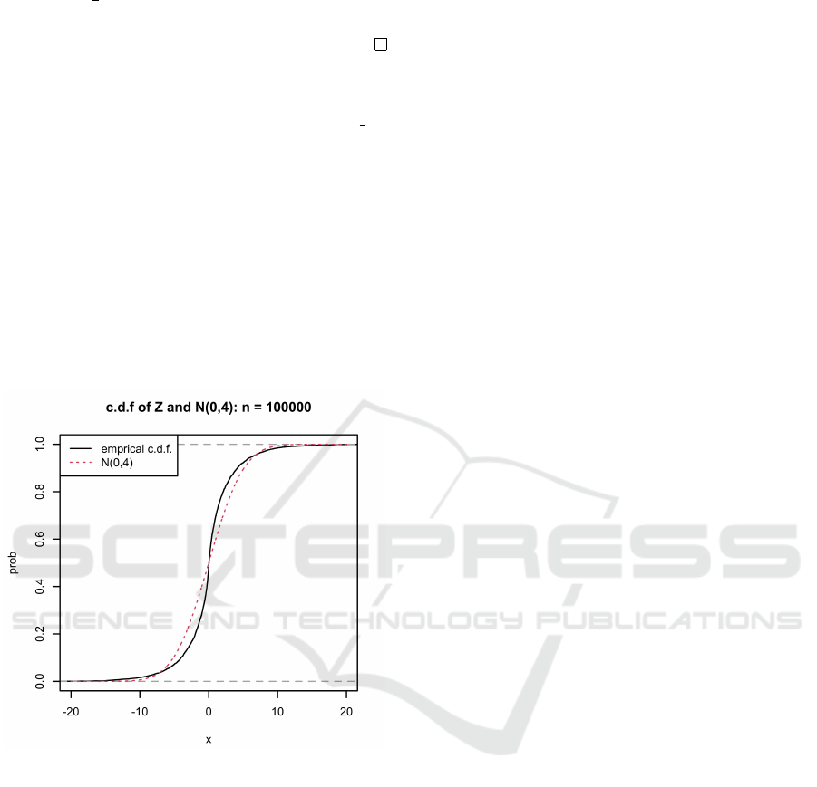
3.2.3 Experimental Veriﬁcation

We showed in Theorem 3.3 that z :=

(|F

−|F

)

distributes according to N (0,4) when n is sufﬁciently

large. We now empirically verify how accurately z

distributes according to N (0, 4) when we set n =

100000. We generate 5000 sets of input sequences

,.. .,x

n−1

iid

∼ U({−1, 1}) by the default PRNG in

R (Comprehensive R Archive Network, 2022), and

then calculate 5000 samples of z. Fig. 1 shows the

empirical c.d.f. of the samples of z and the theoretical

c.d.f. of N (0, 4). We can observe that they match

well, although not perfectly. It is sufﬁcient to con-

clude that z = O(1), which is required for the proof of

Corollary 3.4.

Figure 1: Experimental veriﬁcation of Theorem 3.3.

4 CONCLUSION

Iwasaki (Iwasaki, 2020) proposed a novel analysis to

solve the long-standing problem of the DFT test under

the 3 heuristic assumptions described in Sect. 1.2. In

this paper, we showed that Assumption 2, which is

also required for Assumption 3, holds when n is suf-

ﬁciently large. The rest of the heuristic assumptions

remain unproved, and they remain future work.

REFERENCES

Bassham III, L. E., Rukhin, A. L., Soto, J., Nechvatal, J. R.,

Smid, M. E., Barker, E. B., Leigh, S. D., Levenson,

M., Vangel, M., Banks, D. L., et al. (2010). Sp

800-22 rev. 1a. a statistical test suite for random and

pseudorandom number generators for cryptographic

applications.

Comprehensive R Archive Network (2022). R: The r project

for statistical computing. https://www.r-project.org/.

Hamano, K. (2005). The distribution of the spectrum for the

discrete fourier transform test included in sp800-22.

IEICE Transactions on Fundamentals of Electronics,

Communications and Computer Sciences, 88(1):67–

73.

Iwasaki, A. (2020). Deriving the variance of the discrete

fourier transform test using parseval’s theorem. IEEE

Transactions on Information Theory, 66(2):1164–

1170.

Kim, S.-J., Umeno, K., and Hasegawa, A. (2003). On the

nist statistical test suite for randomness. TECHNICAL

REPORT OF IEICE, 103(499):21–27.

Kim, S.-J., Umeno, K., and Hasegawa, A. (2004). Correc-

tions of the nist statistical test suite for randomness.

Okada, H. and Umeno, K. (2017). Randomness evalu-

ation with the discrete fourier transform test based

on exact analysis of the reference distribution. IEEE

Transactions on Information Forensics and Security,

12(5):1218–1226.

Pareschi, F., Rovatti, R., and Setti, G. (2012). On statistical

tests for randomness included in the nist sp800-22 test

suite and based on the binomial distribution. IEEE

Transactions on Information Forensics and Security,

7(2):491–505.

Rukhin, A., Soto, J., Nechvatal, J., Smid, M., Barker,

E., Leigh, S., Levenson, M., Vangel, M., Banks, D.,

Heckert, A., et al. (2010). Nist special publication

800-22: a statistical test suite for the validation of ran-

dom number generators and pseudo random number

generators for cryptographic applications.

ICISSP 2023 - 9th International Conference on Information Systems Security and Privacy

372