Machine Learning Algorithms for Mouse LFP Data Classification in

Epilepsy

Antonis Golfidis

, Michael Vinos

2,3 a

, Nikos Vassilopoulos

2,3

, Eirini Papadaki

2,3

Irini Skaliora

1,2,3 b

and Vassilis Cutsuridis

1,4 c

Athens International Master’s Programme in Neurosciences, Department of Biology,

National and Kapodistrian University of Athens, Athens, Greece

Department of History and Philosophy of Science, National and Kapodistrian University of Athens, Athens, Greece

Center for Basic Research, Biomedical Research Foundation of the Academy of Athens, Athens, Greece

School of Computer Science, University of Lincoln, Lincoln, U.K.

Keywords: Machine Learning, Classification, HCTSA, Epilepsy, Animal, LFP, Endogenous Activity, Interictal Activity,

Seizure like Activity.

Abstract: Successful preictal, interictal and ictal activity discrimination is extremely important for accurate seizure

detection and prediction in epileptology. Here, we introduce an algorithmic pipeline applied to local field

potentials (LFPs) recorded from layers II/III of the primary somatosensory cortex of young mice for the

classification of endogenous (preictal), interictal, and seizure-like (ictal) activity events using time series

analysis and machine learning (ML) models. Using the HCTSA time series analysis toolbox, over 4000

features were extracted from the LFPs after applying over 7700 operations. Iterative application of correlation

analysis and random-forest-recursive-feature-elimination with cross validation method reduced the

dimensionality of the feature space to 22 features and 27 features, in endogenous-to-interictal events

discrimination, and interictal-to-ictal events discrimination, respectively. Application of nine ML algorithms

on these reduced feature sets showed preictal activity can be discriminated from interictal activity by a radial

basis function SVM with a 0.9914 Cohen kappa score with just 22 features, whereas interictal and seizure-

like (ictal) activities can be discriminated by the same classifier with a 0.9565 Cohen kappa score with just

27 features. Our preliminary results show that ML application in cortical LFP recordings may be a promising

research avenue for accurate seizure detection and prediction in focal epilepsy.

1 INTRODUCTION

Epilepsy, the sacred disease, is one of the oldest

recognizable neurological conditions with written

records dating back to 2000 BCE (Chang and

Lowenstein, 2003; Magiorkinis et al., 2010). As of

2020 around 50 million people worldwide were

affected by epilepsy (Ghosh et al., 2021). The causes

of epilepsy are mostly unknown (idiopathic), but

often epilepsy is caused from brain damage, stroke,

and trauma (Goldberg and Coulter, 2013). The

disease is characterized by recurrent violent episodes

of involuntary movements called seizures, which may

be partial (involve only one part of the body) or

https://orcid.org/0000-0001-9961-1079

https://orcid.org/0000-0002-7528-7208

https://orcid.org/0000-0001-9005-0260

generalized (involve the whole body) followed at

times by loss of consciousness and/or control of

bowel or bladder function (Duncan et al., 2006).

Seizures are the result of excessive electrical

discharges in neuronal populations (Colmers and

Maguire, 2020). Seizures measured by

electroencephalography (EEG) or LFP recordings

have been shown to vary in frequency, from one per

year to several episodes per day. Because they occur

so sporadically and at unknown times, the availability

of seizure-like (ictal) activity is scarce and thus

interictal activity is often used in diagnosis.

The best way for detecting interictal activity is a

visual inspection of the EEG/LFP signal by an expert

Golﬁdis, A., Vinos, M., Vassilopoulos, N., Papadaki, E., Skaliora, I. and Cutsuridis, V.

Machine Learning Algorithms for Mouse LFP Data Classiﬁcation in Epilepsy.

DOI: 10.5220/0011625600003414

In Proceedings of the 16th International Joint Conference on Biomedical Engineering Systems and Technologies (BIOSTEC 2023) - Volume 4: BIOSIGNALS, pages 36-47

ISBN: 978-989-758-631-6; ISSN: 2184-4305

 2023 by SCITEPRESS – Science and Technology Publications, Lda. Under CC license (CC BY-NC-ND 4.0)

(Lodder et al., 2014). This approach, however, has

several limitations including a very long learning

curve and extensive analysis time, especially for long

recordings. Human error, subjectivity, intra and

interobserver variability often result in misdiagnosis

leading to lack of treatment or prescription of

medication with potentially harmful side effects

(Lodder et al., 2014).

Overcoming these drawbacks requires the

development of an artificial intelligence system for an

automatic pre-ictal, interictal, and ictal detection that

can match or even outperform experts, hence

reducing the time and resources spent on visual

analysis, as well as misdiagnosis rates.

Herein, we introduce an algorithmic pipeline

applied to LFP signals recorded from mouse

somatosensory cortical slices to extract features used

for the classification of endogenous (preictal),

interictal, and seizure-like (ictal) events using time

series analysis and ML models.

2 MATERIALS AND METHODS

2.1 LFP Data

2.1.1 Animals

Thirty-one C57Bl/6J mice were bred in the animal

facility of the Center for Experimental Surgery of the

Biomedical Research Foundation of the Academy of

Athens, registered as a breeding and experimental

facility according to the Presidential Decree of the

Greek Democracy 160/91, which harmonizes the

Greek national legislation with the European Council

Directive 86/609/EEC on the protection of animals

used for experimental and other scientific purposes.

The present study was approved by the Regional

Veterinary Service, in accordance with the National

legal framework for the protection of animals used for

scientific purposes (reference number 2834/08-05-

2013). Mice were weaned at 21 days old, housed in

groups of 5 – 7, in 267 × 483 × 203 mm cages

supplied with bedding material and kept at a 12/12 h

dark-light schedule. Food was provided ad libitum.

2.1.2 Slice Preparation

Coronal brain slices (400 μm) were prepared from the

primary somatosensory cortex of young mice (P18-

20) as described before (Rigas et al 2015; 2018;

Sigalas et al 2015; 2017). Briefly slices were placed

in a holding chamber with artificial cerebrospinal

fluid (ACSF) containing (in mM): NaCl 126; KCl

3.53; NaH2PO4.H2O 1.25; NaHCO3 26; MgSO4 1;

D-Glucose 10 and CaCl2.2H2O 2 [osmolarity (mean

± SD): 317 ± 4 mOsm, pH: 7.4±0.2], where they were

left to recover at room temperature (RT: 24–26 °C).

2.1.3 ex Vivo Electrophysiology

Twenty minutes LFP recordings of endogenous

cortical activity in the form of recurring Up and Down

states were obtained. Subsequently, epileptiform

activity was induced by replacing the ACSF with low

ACSF (Avoli & Jefferys, 2016; Dreier &

Heinemann, 1991) for up to 80 minutes to ensure that

the pattern of epileptiform activity had stabilized.

Network activity was assessed by LFP recordings

which were obtained from cortical layers II/III of

S1BF using low impedance (∼0.5 MΩ) glass pipettes

filled with ACSF. Recordings were obtained in

current-clamp mode with a Multiclamp 700B

amplifier (Molecular Devices, San Jose, CA, USA).

LFP signals were low-pass filtered at 6 kHz (by an

analog anti-aliasing filter) and subsequently digitized

at 15 kHz by means of a 16-bit multi-channel

interface (InstruTECH ITC-18; HEKA Elektronic,

Lambrecht, Germany). Data acquisition was

accomplished using AxoGraph X (version 1.3.5;

https://axograph.com; RRID: SCR_014284).

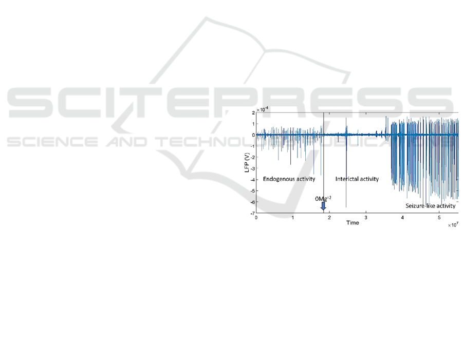
Figure 1: Exemplary 20-min LFP recording trace from a

coronal slice of the primary somatosensory cortex of a

young mouse. Blue downward pointing arrow indicates the

time the ACSF was replaced with zero Mg

ACSF.

2.1.4 Data Analysis

The detection of spontaneous network events was

performed semi-automatically from the LFP

recordings. Traces were exported to MATLAB

format and analyzed with LFPAnalyzer, an in-house-

developed software (Tsakanikas et al., 2017;

Kaplanian et al., 2022). Briefly: (i) input signals were

pre-processed by DC offset subtraction and low-pass

filtering at 200 Hz; (ii) two feature sequences were

extracted for each segment, based on two

Machine Learning Algorithms for Mouse LFP Data Classiﬁcation in Epilepsy

complementary mathematical transformations

(Hilbert and Short energy); (iii) a dynamic, data-

driven threshold based on Gaussian mixture models

was estimated for each feature sequence and used to

create a mask; and (iv) the two masks were combined

using a logical OR operator and used for the detection

of the onset and offset of the LFP events. After

identification of their onset and offset, events were

manually classified as endogenous activity (EA) (up-

states), interictal activity (IA), or seizure-like activity

(SLA) (see Figure 1 for traces of these three types of

events) based on their shape (waveform), and on the

basis of previous simultaneous whole-cell patch

clamp recordings (Sigalas et al 2015; Kaplanian et al

2022).

2.2 Algorithmic pipeline

Our high-level algorithmic pipeline is depicted in

Figure 2. Every step in the pipeline is described in

detail in the following sections.

Figure 2: General algorithmic pipeline.

2.2.1 Data Preparation

The steps followed for preparing the data for further

analysis are depicted in Figure 3.

Figure 3: Data preparation pipeline.

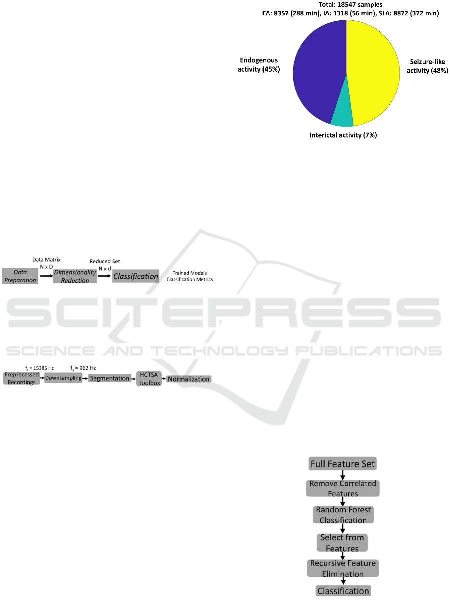
All digitized recordings were downsampled (f

= 962

Hz). A segmentation window with a 5 sec duration

and a 50% overlap was slid to all signals to segment

them into 18542 samples. Out of these samples 8357

were identified as EA, 1318 as IA and 8872 as SLA

by expert users (see Figure 4 for segmented data

distributions). The HCTSA suite of time series

methods (Fulcher et al., 2013) was then used to

extract features. HCTSA consists of thousands of

time-series analysis methods allowing users to

convert a time series into a vector of thousands of

informative features, corresponding to different

outputs of time-series analysis operations (Fulcher et

al., 2013; Fulcher and Jones, 2017). HCTSA has been

successfully used to a wide range of problems

including the diagnosis of Parkinson’s disease from

speech signals, monitoring sleep-stage progression,

predicting schizophrenia from brain imaging data,

Figure 4: Segmented signal events distribution. EA:

endogenous activity; IA: interictal activity; SLA: seizure-

like activity. Time in parenthesis is the total cumulative

duration of each event class in minutes.

and forecasting catastrophes in financial and

ecological systems. The features we extracted with

HCTSA were from the time, frequency, time-

frequency, and chaotic domains of the segmented

LFP signals by performing over 7700 operations to

them. For all segmented signals from our LFP

recordings a total of 4476 meaningful (non-zero, non-

constant, etc) features were extracted. All features

were then normalized to a common scale (0-1),

without distorting differences in the ranges of values.

These features constituted the Full Feature Set.

2.2.2 Dimensionality Reduction

The steps followed for reducing the dimensionality of

the extracted features of the LFP data are depicted in

Figure 5. To further reduce the high-dimensional

space of the extracted features we calculated the

correlation scores of all features in the Full Feature

Set. Any features whose score was higher than ρ were

removed. The remaining features constituted the

Uncorrelated Feature Set.

Figure 5: Dimensionality reduction pipeline.

BIOSIGNALS 2023 - 16th International Conference on Bio-inspired Systems and Signal Processing

On the uncorrelated feature set we used Random

Forrest (RF) (Breiman, 2001), a machine learning

method that operates by constructing a multitude of

decision trees at training time (Ho, 1995, 1998). For

classification tasks, RF performs implicit feature

selection, using a small subset of "strong variables"

for classification only, resulting in superior

performance on high-dimensional data (Menze et al,

2009). The mean decrease of Entropy (or increase of

Information Gain) over all the decision trees is an

indicator of feature relevance derived from this

implicit feature selection of the random forest. A

feature importance score indicates the relative

importance of features, which is a by-product of

random forest classifier training. Several studies

(Menze et al., 2007; Díaz-Uriarte & Alvarez de

Andres, 2006) have shown that this feature selection

step can significantly reduce the number of features

while increasing the model’s accuracy. The output of

RF is the class selected by most trees according to

some predefined criterion (Ho, 1998). The criterion in

our case was the importance score (we kept those

features with score greater than 6*mean importance

score). Each of these feature sets constituted the

Selected Features Set. A recursive feature elimination

with cross-validation (RFECV) method was then

used to remove the weakest features and find from

each Selected Features Set the optimum number of

features that gave the best accuracy results. Because

it was not known in advance how many features

would be valid, cross validation was used with RFE

to score different feature subsets and find the average

optimum number of features. Each of these optimum

number of features constituted the RFE Feature Set.

2.2.3 Classification

We employed 9 machine learning classifiers: a linear

SVM (SVMlin), a polynomial of the 2

degree SVM

(SVMpol), a polynomial of the 3

degree SVM

(SVMpol), a polynomial of the 4

degree SVM

(SVMpol), a polynomial of the 5

degree SVM

(SVMpol), a radial basis function with a Gaussian

kernel SVM (SVMrbf), an RF, a decision tree (DT)

and a k-nearest neighbours (kNN). The data (N

samples x M features) were split into a training set

(80%) and a validation test set (20%). A stratified 5-

fold cross validation was used to preserves the

percentages of samples of each fold. A

GridSearchCV function was used for hyperparameter

tuning of every classifier (see Table 1).

Table 1: Machine learning classifiers, their

hyperparameters and their hyperpameter values. C:

Controls the amount of misclassified data points allowed by

introducing a penalty. Low C values lead to decision

boundaries with large margin. High C values add greater

penalty thus minimizing the number of misclassified

examples; Gamma: The distance of influence of a training

point. Low values of gamma indicate greater distance

resulting in more points taken into account for the

calculation of the separation line; N_estimators (RF): The

number of decision trees being built in the forest;

Max_depth (RF): The number of splits that each decision

tree is allowed to make; N_estimators (kNN): The number

of nearest neighbors; Criterion (DT): How the impurity of

a split will be measured; Max_depth (DT): The number of

splits that the decision tree is allowed to make.

Classifier Hyperparameter Values

SVMlin C [0.01, 0.1, 1, 10]

SVMpol (2

degree)

C [0.01, 0.1, 1, 10]

SVMpol (3

degree)

C [0.01, 0.1, 1, 10]

SVMpol (4

degree)

C [0.01, 0.1, 1, 10]

SVMpol (5

degree)

C [0.01, 0.1, 1, 10]

SVMrbf C [0.01, 0.1, 1, 10]

Gamma [0.1, 1, 10]

RF N_estimators [100, 200, 300,

400, 500, 600,

700, 800, 900]

Max_depth [10, 20, 30]

DT Criterion [gini, entropy]

Max_depth

[1, 2, 3, 4, 5, 10,

20, 30]

kNN N_estimators [1, 2, 3, 4, 5, 6,

7, 8, 9, 10]

Performance Metrics. We used the following

metrics for evaluating the performances of our

classifiers:

𝐶𝑜ℎ𝑒𝑛 𝜅 =

 (∗∗)

(



)

∗

(



)



(



)

∗()

𝑃𝑟𝑒𝑐𝑖𝑠𝑖𝑜𝑛 =





𝑅𝑒𝑐𝑎𝑙𝑙 =





𝐹1 𝑠𝑐𝑜𝑟𝑒 = 2 ∗

∗



where TP are the true positives, TN are the true

negatives, FP are the false positives and FN are the

Machine Learning Algorithms for Mouse LFP Data Classiﬁcation in Epilepsy

false negatives. The Cohen kappa score was used

because our classes (EA, IA and SLA) were

unbalanced. The Cohen kappa score values ranged

from -1 (worst) to +1 (best). The Precision, Recall,

and F1-score values ranged from 0 (worst) and 1

(best).

3 RESULTS

3.1 EA vs IA Classification

We started our analysis from the downsampled and

segmented 9674 samples (8357 EA + 1318 IA) and

applied the HCTSA toolbox on them to extract 4476

meaningful features (Full Feature Set). Then, starting

with the full feature set we followed the

“Dimensionality Reduction” pipeline depicted in

figure 5 and described in section 2.2.2. In every step

of this pipeline, we evaluated the performances of all

nine classifiers to determine how much of the

performance will be lost as the feature space is

reduced. The performances of all nine classifiers

tested against the Full Feature Set are summarized in

Table 2. We then calculated the correlation score of

each feature in the full feature set, compared it to the

ρ criterion (see section 2.2.2 for details) and kept only

those features whose correlation score was lower than

ρ. We tried different values for ρ (ρ = 0.8 or ρ = 0.9).

We kept ρ = 0.9 because it gave the best Cohen kappa

scores when only an RF was tested against the derived

number of features (1933 features). These 1933

features constituted the Uncorrelated Feature Set.

We tested the performances of our classifiers

including the RF one on the Uncorrelated Feature Set

and found that SVMpol of the 2

degree had the best

Cohen kappa score (see Table 3). In the next step and

to further reduce the feature space we employed the

RF with a criterion method (we kept those features

with score greater than 6*mean importance score =

0.0031) on the uncorrelated feature set to find the 62

most important features (Selected Features Set). We

tested once again the performances of our classifiers

on the Selected Features Set. The SVMrbf displayed

the best performance (Cohen kappa score = 0.98,

precision = 0.9893, recall = 0.9893, F1-score =

0.9893) (see Table 4). Finally, the RFECV method

was employed to find the optimum feature set (RFE

Feature Set). RFECV resulted in 31 optimum

features. Once more we tested performances of our

classifiers on this feature set and found that the best

performance was SVMrbf (Cohen kappa score =

0.9871, precision = 0.9951, recall = 0.9920, F1-score

= 0.9936) (see Table 5).

Table 2: Classifiers’ performances on the full feature set

(4476 features).

Classifier

Cohen

kappa

Precision Recall

F1-

score

SVMlin 0.959 0.9833 0.9758 0.9795

SVMpol

degree

0.9678 0.9861 0.9817 0.9839

SVMpol

degree

0.9657 0.9841 0.9814 0.9828

SVMpol

degree

0.9657 0.9843 0.9814 0.9828

SVMpol

degree

0.9613 0.9836 0.9777 0.9806

SVMrbf - - - -

RF 0.9316 0.9658 0.9658 0.9658

kNN 0.9027 0.9564 0.9465 0.9513

DT 0.9056 0.9542 0.9514 0.9528

Table 3: Classifiers’ performances on the uncorrelated

feature set (1933 features).

Classifier

Cohen

kappa

Precision Recall

F1-

score

SVMlin 0.9461 0.9768 0.9694 0.9731

SVMpol

degree

0.9590 0.9833 0.9758 0.9795

SVMpol

degree

0.9611 0.9851 0.9761 0.9806

SVMpol

degree

0.9568 0.9829 0.974 0.9784

SVMpol

degree

0.9524 0.9823 0.9703 0.9762

SVMrbf - - - -

RF 0.9275 0.9769 0.9516 0.9638

kNN 0.9105 0.9649 0.9462 0.9553

DT 0.8460 0.9230 0.9230 0.9230

Table 4: Classifiers’ performances on the selected feature

set (62 features).

Classifier

Cohen

kappa

Precision Recall

F1-

score

SVMlin 0.9202 0.9637 0.9566 0.9601

SVMpol

degree

0.9367 0.9783 0.959 0.9684

SVMpol

degree

0.9674 0.9772 0.9801 0.9787

SVMpol

degree

0.9617 0.9780 0.9838 0.9809

SVMpol

degree

0.9660 0.9801 0.986 0.983

SVMrbf 0.9786 0.9893 0.9893 0.9893

RF 0.9654 0.9888 0.9767 0.9827

kNN 0.9491 0.9703 0.9789 0.9746

DT 0.8736 0.9375 0.9361 0.9368

BIOSIGNALS 2023 - 16th International Conference on Bio-inspired Systems and Signal Processing

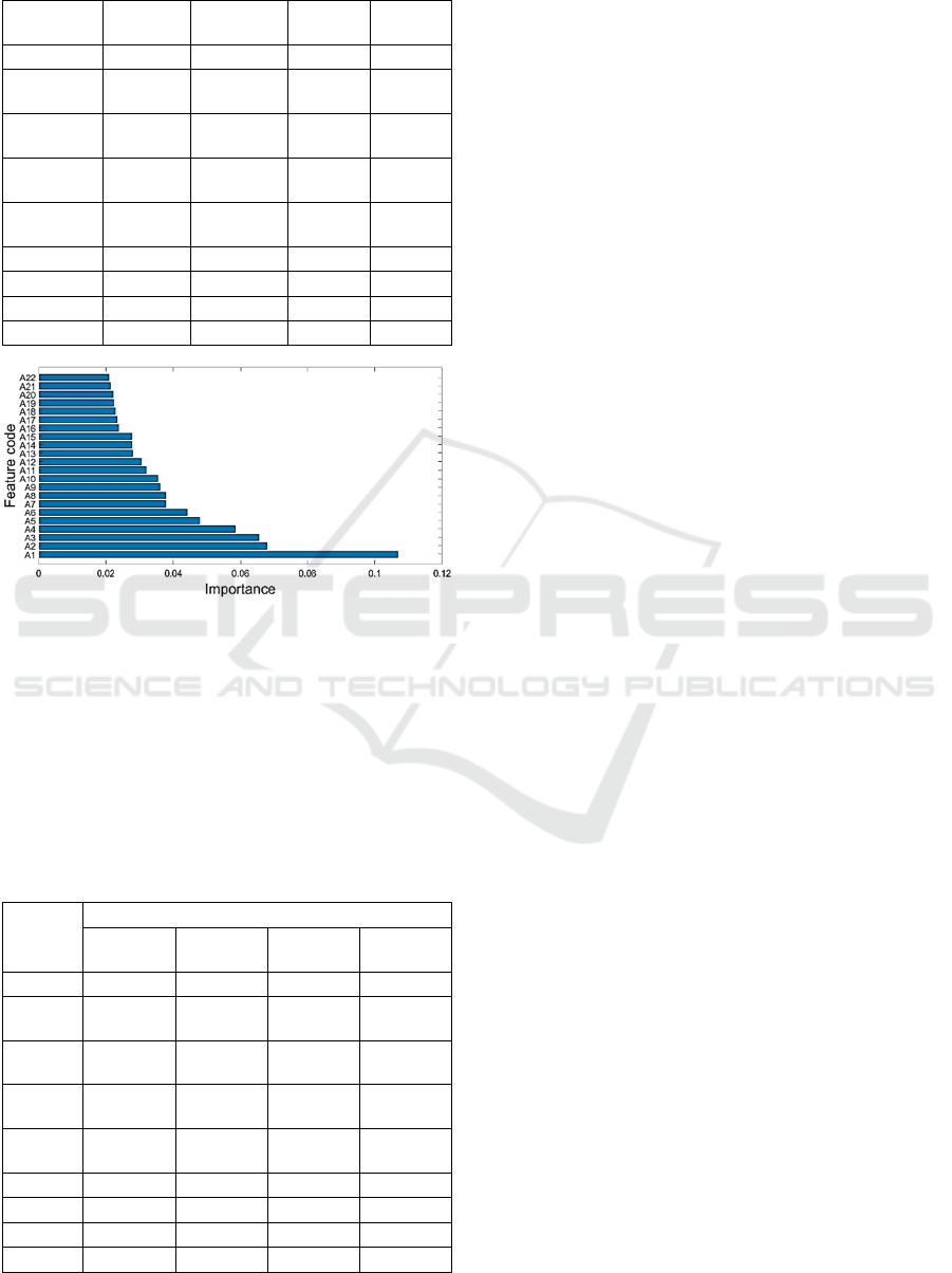
Table 5: Classifiers’ performances on the RFE feature set

(31 features).

Classifier Cohen

kappa

Precision Recall F1-

score

SVMlin 0.9295 0.9641 0.9655 0.9648

SVMpol

degree

0.8890 0.9628 0.9281 0.9445

SVMpol

degree

0.9638 0.9797 0.9841 0.9819

SVMpol

degree

0.9700 0.9865 0.9835 0.985

SVMpol

degree

0.9677 0.9876 0.9801 0.9838

SVMrbf 0.9871 0.9951 0.9920 0.9936

RF 0.9740 0.9932 0.9810 0.9870

kNN 0.9680 0.9832 0.9847 0.9840

DT 0.8954 0.9470 0.9484 0.9477

Figure 6: Importance scores of all 22 features in the RFE

feature set. See appendix for description of each feature

code.

Figure 6 depicts the importance scores of the 22 out

of the 31 features from the RFE feature set. See

Appendix for detailed description of each coded

feature in Fig. 6. The bottom feature has the highest

importance score value (IS > 0.1). We then

Table 6: Classifiers’ Cohen kappa scores on the RFE

feature set for different IS values. IS: importance score.

Classifier Cohen kappa score

IS > 0.02

(22 features)

IS > 0.03

(12 features)

IS > 0.04

(6 features)

IS > 0.05

(4 features)

SVMlin 0.9146 0.8597 0.7361 0.6113

SVMpol

degree

0.9328 0.9128 0.8348 0.6015

SVMpol

degree

0.9722 0.9442 0.8780 0.6078

SVMpol

degree

0.9722 0.9464 0.8941 0.6031

SVMpol

degree

0.9659 0.9440 0.9064 0.5908

SVMrbf 0.9914 0.9525 0.9073 0.6300

RF 0.9761 0.9566 0.9241 0.7518

kNN 0.9724 0.9534 0.9059 0.7202

DT 0.9033 0.9028 0.9059 0.6932

investigated combinations of these features to see if

we can improve the performances of our classifiers

and to also assess when their performances worsen as

feature space is further reduced. These results (Table

6) reveal that almost all classifiers’ performances

improved (compare values in Tables 5 and 6).

SVMrbf had an almost perfect Cohen kappa score

(0.9914) for 22 features. For smaller number of

features all classifiers’ Cohen kappa scores

progressively became worse (see Table 6).

3.2 IA vs SLA Classification

For the binary classification of IA vs SLA, we started

our analysis from the downsampled and segmented

10190 samples (8872 SLA + 1318 IA) and applied the

HCTSA toolbox on them to extract 4476 meaningful

features (Full Feature Set). We followed the

“Dimensionality Reduction” pipeline depicted in

figure 5 and described in section 2.2.2. In every step

of this pipeline, we evaluated the performances of our

nine classifiers to determine how they were affected

as the feature space was reduced. The classifiers’

performances on the Full Feature Set are summarized

in Table 7. As before we then calculated the

correlation score of each feature in the Full Feature

Set, compared it to the ρ criterion (see section 2.2.2

for details) and kept only those features whose

correlation score was lower than ρ. We tried different

values for ρ (0.8 and 0.9) and kept ρ = 0.9 because it

gave the best Cohen kappa scores when only an RF

was tested against the derived number of features

(1944 features). These 1944 features constituted the

Uncorrelated Feature Set. We tested the

performances of our classifiers including the RF one

on this reduced set and found that SVMpol of the 5

degree had the best Cohen kappa score (see Table 8).

Next, we employed the RF with a criterion method

(kept as before those features with score greater than

6*mean importance score = 0.0031) on the

Uncorrelated Feature Set to find the 40 most

important features (Selected Features Set). We tested

once again the performances of our classifiers on the

Selected Features Set. The SVMrbf had the best

performance (Cohen kappa score = 0.9217, precision

= 0.9849, recall = 0.9399, F1-score = 0.9608) (see

Table 9). Finally, the RFECV method was employed

to find the optimum feature set (RFE Feature Set).

RFECV resulted in 27 optimum features. We tested

again the performances of the nine classifiers on this

feature set and found that the best performance was

still SVMrbf (see Table 10).

Machine Learning Algorithms for Mouse LFP Data Classiﬁcation in Epilepsy

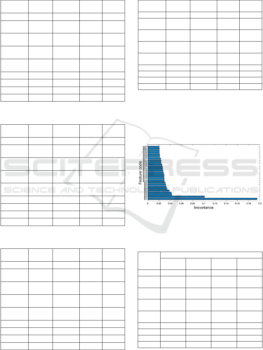
Table 7: Classifiers’ performances on the full feature set

(4476 features).

Classifier

Cohen

kappa

Precision Recall

F1-

score

SVMlin 0.7675 0.8991 0.8699 0.8837

SVMpol

degree

0.8003 0.9227 0.8807 0.9001

SVMpol

degree

0.8112 0.9293 0.8852 0.9056

SVMpol

degree

0.8298 0.9373 0.8953 0.9148

SVMpol

degree

0.8253 0.935 0.8932 0.9226

SVMrbf - - - -

RF 0.8157 0.9702 0.86 0.9076

kNN 0.7649 0.8985 0.8680 0.8824

DT 0.7379 0.8713 0.8666 0.8690

Table 8: Classifiers’ performances on the uncorrelated

feature set (1944 features).

Classifier

Cohen

kappa

Precision Recall

F1-

score

SVMlin 0.7222 0.8770 0.8470 0.8611

SVMpol

degree

0.7573 0.9007 0.8596 0.8796

SVMpol

degree

0.7524 0.9082 0.8502 0.876

SVMpol

degree

0.7760 0.9193 0.8625 0.8879

SVMpol

degree

0.7837 0.9271 0.8636 0.8917

SVMrbf - - - -

RF 0.7663 0.9697 0.8291 0.8826

kNN 0.7751 0.8852 0.89 0.8876

DT 0.7369 0.8852 0.8736 0.8684

Table 9: Classifiers’ performances on the selected feature

set (40 features).

Classifier

Cohen

kappa

Precision Recall

F1-

score

SVMlin 0.7503 0.9019 0.8528 0.8750

SVMpol

degree

0.9145 0.9704 0.945 0.9572

SVMpol

degree

0.9089 0.9619 0.9473 0.9545

SVMpol

degree

0.9133 0.9641 0.9495 0.9566

SVMpol

degree

0.9147 0.9689 0.9466 0.9574

SVMrbf 0.9217 0.9849 0.9399 0.9608

RF 0.9154 0.9788 0.9390 0.9577

kNN 0.8905 0.9573 0.9341 0.9453

DT 0.7942 0.9078 0.8871 0.8971

Table 10: Classifiers’ performances on the RFE feature set

(27 features).

Classifier Cohen

kappa

Precision Recall F1-

score

SVMlin 0.6773 0.8853 0.8046 0.8383

SVMpol

degree

0.9219 0.9685 0.9537 0.961

SVMpol

degree

0.9158 0.9631 0.9529 0.9579

SVMpol

degree

0.9206 0.9625 0.9582 0.9603

SVMpol

degree

0.9203 0.9639 0.9566 0.9602

SVMrbf 0.9565 0.9878 0.9692 0.9782

RF 0.9227 0.9781 0.9462 0.9614

kNN 0.9209 0.9746 0.9475 0.9605

DT 0.7981 0.9016 0.8965 0.899

Figure 8 depicts the importance scores of all 27

features from the RFE Feature Set. See Appendix for

detailed description of each coded feature in Fig. 8.

The bottom feature has the highest importance score.

We investigated combinations of these features to see

if we can further improve the classification

performance of our classifiers and also when their

Figure 8: Importance scores of all 27 features in the RFE

feature set. See appendix for description of each feature

code.

Table 11: Classifiers’ Cohen kappa scores on the RFE

feature set for different IS values. IS: importance score.

Classifier Cohen kappa score

IS > 0.02

(27 features)

IS > 0.03

(9 features)

IS > 0.04

(4 features)

IS > 0.05

(2 features)

SVMlin 0.6773 0.2969 - -

SVMpol

degree

0.9219 0.8457 0.3829 -

SVMpol

degree

0.9158 0.8730 0.3565 0.1438

SVMpol

degree

0.9206 0.8932 0.4522 0.2079

SVMpol

degree

0.9204 0.8856 0.4860 0.2963

SVMrbf 0.9565 0.9080 0.7410 0.6523

RF 0.9227 0.9054 0.7749 0.6036

kNN 0.9209 0.8942 0.7258 0.6572

DT 0.7981 0.8227 0.7491 0.5969

BIOSIGNALS 2023 - 16th International Conference on Bio-inspired Systems and Signal Processing

performance worsen as feature space is further

reduced. These results are depicted in Table 11. As the

number of features decreased all classifiers’ Cohen

kappa score progressively become worse. kNN had the

best score (0.6572) with only two features.

4 DISCUSSION

Our study has produced several interesting results

concerning the usefulness of time series analysis and

ML in LFP based epileptology. Most importantly it

showed that discriminating endogenous (pre-ictal)

activity from interictal activity is more successful

(and easier) than discriminating interictal from

seizure-like (ictal) activity. This result confirms past

research findings (Fischer, 2014). By using feature

extraction methods from the time, frequency, time-

frequency and chaotic domains and standard (single

and ensemble) ML methods such as kNN, RF, SVM,

and DT we achieved an over 0.9 Cohen kappa score

and an over 0.95 precision and recall scores when the

Full Feature Set (4476 features) was used in the EA

vs IA discrimination task. As the feature space was

reduced (4476 to 22) the discriminability of the ML

classifiers changed. The classifier with the best

performance was SVMrbf (Cohen kappa score =

0.9914), whereas the classifier with the worst

performance was DT (Cohen kappa score = 0.9033).

The average Cohen kappa score was 0.96. Out of the

22 most important features, the feature with the

highest importance score (IS ~ 0.12) was the ratio of

autocorrelation (using lag = 2) of the transformed

time series over the original time series when 5% of

time points closest to the mean were removed. When

only the first 4 features with the highest importance

scores (A1-A4 in Fig. 6) were used, then the

discriminability of the classifiers ranged from 0.59-

0.75 (Average Cohen kappa score = 0.6455).

Addition of just two more features (4 to 6) increased

the performances of the classifiers by 23% on average

(Average Cohen kappa score = 0.8769). Addition of

6 more features (6 to 12) increased the performances

of the classifiers by only 5% (Average Cohen kappa

score = 0.9302).

In the interictal vs seizure-like (ictal) activity

discrimination task the landscape was different. As

before using feature extraction methods from the

time, frequency, time-frequency and chaotic domains

and the same ML methods we achieved an over 0.73

Cohen kappa score, an over 0.87 precision score, and

an over 0.86 recall score when the Full Feature Set

(4476 features) was used. As the feature space was

reduced (4476 to 27) the discriminability of the ML

classifiers changed. The classifier with the best

performance was once again the SVMrbf (Cohen

kappa score = 0.9565), whereas the classifier with the

worst performance was SVMlin (Cohen kappa score =

0.6773). The average Cohen kappa score was 0.88. Out

of the 27 most important features, the feature with the

highest importance score (IS > 0.19) was the mean

power spectrum density. When only the first 2 features

with the highest importance scores (A1-A2 in Fig. 8)

were used, then the discriminability of the classifiers

ranged from 0.14-0.65 (Average Cohen kappa score =

0.45). Addition of just two more features (2 to 4)

increased the performances of the classifiers by 13%

on average (Average Cohen kappa score = 0.58).

Addition of 5 more features (4 to 9) the inverse effect

to EA vs IA was seen: the average performance of the

classifiers increased by an additional 23% (Average

Cohen kappa score = 0.8103).

From these results it is evident that even though in

both discrimination tasks the first feature had a much

higher importance score than other features in the set

(see Figs 6 and 8), on each own it was not enough to

discriminate the pre-ictal (endogenous) from the

interictal, and the interictal from the ictal (seizure-

like) events. The performances of the classifiers on

average were poor (not shown here). Thus, the

discrimination ability of the classifiers depends on the

cumulative effect of the features, and not on the

individual effect of each feature. It is yet to be

determined whether this cumulative effect is additive

or multiplicative.

5 CONCLUSIONS

A novel algorithmic pipeline was successfully

applied to LFP recordings from layers II/III of the

primary somatosensory cortex of young mice to

discriminate with high accuracy the endogenous

(preictal), interictal and seizure-like (ictal) activity

events using time series analysis and ML modelling.

Over 4000 features were successfully extracted using

over 7700 operations applied to the LFPs. The high

dimensionality of the feature space was then reduced

via an iterative process of correlation analysis and

RF-RFECV to only 22 features for the EA vs IA

discrimination case and to 27 features for the IA vs

SLA one. ML algorithms were then applied to these

reduced feature sets and a radial basis function SVM

with a Gaussian kernel has been discovered to

discriminate with a 0.99 Cohen kappa score the EA

from IA and with a 0.9565 Cohen kappa the IA and

SLA. Our preliminary results show that ML

application in intracortical LFPs may be a promising

Machine Learning Algorithms for Mouse LFP Data Classiﬁcation in Epilepsy

research avenue for accurate seizure detection and

prediction in focal epilepsy.

ACKNOWLEDGEMENTS

This work was supported by the European Union’s

Horizon 2020 Research and Innovation programme

under the Marie-Sklodowska Curie grant no778062

ULTRACEPT (VC) and the Human Resources and

Development, Education and Lifelong learning

programme no MIS-5049391 (IS).

REFERENCES

Avoli M., Jefferys J.G.R. (2016). Models of drug-induced

epileptiform synchronization in vitro. Journal of

Neuroscience Methods, 260: 26-32

Breiman L. (2001). Random forests. Mach Learn., 45:5–32.

Chang B.S., Lowenstein D.H. (2003). Epilepsy. The New

England Journal of Medicine, 349 (13): 1257–66

Chicco D., Warrens M.J., Jurman G. (2021). The Matthews

Correlation Coefficient (MCC) is More Informative

Than Cohen’s Kappa and Brier Score in Binary

Classification Assessment. IEEE Access, 9:78368-

78381. doi: 10.1109/ACCESS.2021.3084050.

Colmers P.L.W., Maguire J. (2020). Network Dysfunction in

Comorbid Psychiatric Illnesses and Epilepsy. Epilepsy

Curr., 20(4):205-210

Díaz-Uriarte R, Alvarez de Andrés S. (2006). Gene selection

and classification of microarray data using random forest.

BMC Bioinformatics, 7(1): 1-13.

Dreier J.P., Heinemann U. (1991). Regional and time

dependent variations of low Mg

induced epileptiform

activity in rat temporal cortex slices. Experimental Brain

Research, 87(3): 581-596

Duncan J.S., Sander J.W., Sisodiya S.M., Walker M.C.

(2006). Adult epilepsy. Lancet, 367(9516): 1087–1100.

Fischer R. (2014). How can we identify ictal and interictal

abnormal activity? Adv Exp Med Biol., 813: 3–23

Fulcher B.D., Little M.A., Jones N.S. (2013). Highly

comparative time-series analysis: the empirical structure

of time series and their methods. J. Roy. Soc. Interf., 10:

20130048

Fulcher B.D., Jones N.S. (2017). hctsa: A Computational

Framework for Automated % Time-Series Phenotyping

Using Massive Feature Extraction. Cell Systems, 5: 527.

Ghosh S., Sinha J.K., Khan T., Devaraju K.S., Singh P.,

Vaibhav K., Gaur P. (2021). Pharmacological and

Therapeutic Approaches in the Treatment of Epilepsy.

Biomedicines, 9 (5): 470.

Goldberg E.M., Coulter D.A. (2013). Mechanisms of epile-

ptogenesis: a convergence on neural circuit dysfunction.

Nature Reviews Neuroscience 14 (5): 337–49.

Ho T.K. (1995). Random Decision Forests. In Proceedings

of the 3rd International Conference on Document

Analysis and Recognition, Montreal, QC, 14–16 August

1995. pp. 278–282.

Ho T.K. (1998). The Random Subspace Method for

Constructing Decision Forests. IEEE Transactions on

Pattern Analysis and Machine Intelligence, 20(8): 832–

844.

Kaplanian A, Vinos M, Skaliora I. (2022). GABAB - and

GABAA -receptor-mediated regulation of Up and Down

states across development. The Journal of Physiology,

600(10): 2401-2427.

Lodder S.S., Askamp J., van Putten M.J. (2014). Computer-

assisted interpretation of the EEG background pattern: a

clinical evaluation. PLoS ONE, 9(1): e85966.

Magiorkinis E., Sidiropoulou K., Diamantis A. (2010).

Hallmarks in the history of epilepsy: epilepsy in

antiquity. Epilepsy Behav., 17(1):103-8

Menze BH, Kelm BM, Masuch R, Himmelreich U, Bachert

P, Petrich W, Hamprecht FA. (2009). A comparison of

random forest and its Gini importance with standard

chemometric methods for the feature selection and

classification of spectral data. BMC bioinformatics,

10(1): 1-16.

Menze BH, Petrich W, Hamprecht FA. (2007). Multivariate

feature selection and hierarchical classification for

infrared spectroscopy: serum-based detection of bovine

spongiform encephalopathy. Anal Bioanalytical Chem,

387(5): 1801-1807.

Rigas P., Adamos D.A., Sigalas C., Tsakanikas P., Laskaris

N.A., Skaliora I. (2015). Spontaneous Up states in vitro:

A single-metric index of the functional maturation and

regional differentiation of the cerebral cortex. Frontiers

in Neural Circuits, 9: 59.

Rigas P., Sigalas C., Nikita M., Kaplanian A., Armaos K.,

Leontiadis L.J., Zlatanos C., Kapogiannatou A., Peta C.,

Katri A., Skaliora I. (2018) Long-Term Effects of Early

Life Seizures on Endogenous Local Network Activity of

the Mouse Neocortex. Front. Synaptic Neurosci., 10:43.

Sigalas C., Rigas P., Tsakanikas P., Skaliora I. (2015). High-

affinity nicotinic receptors modulate spontaneous

cortical up states in vitro. Journal of Neuroscience,

35(32): 11196-208.

Sigalas C., Konsolaki E., Skaliora I. (2017). Sex differences

in endogenous cortical network activity: spontaneously

recurring Up/Down states. Biol Sex Differ, 8:21.

Talkner P., Weber R.O. (2000). Power spectrum and

detrended fluctuation analysis: Application to daily

temperatures. Phys. Rev. E, 62(1): 150

Tsakanikas P., Sigalas C., Rigas P., Skaliora I. (2017). High-

Throughput Analysis of in-vitro LFP Electrophy-

siological Signals: A validated workflow/software

package. Scientific Reports, 7(1):3055

APPENDIX

All Matlab functions used to extract the features

described below are from the HCTSA time series

toolbox (Fulcher et al., 2013, 2017).

BIOSIGNALS 2023 - 16th International Conference on Bio-inspired Systems and Signal Processing

EA vs IA Classification

A1: How time-series properties change as 5% of time

points are removed. The time points being removed

are those that are the closest to the mean. The ratio of

autocorrelation (using lag = 2) of the transformed

time series over the original time series is the

extracted feature. The DN_RemovePoints.m function

was used to extract this feature.

A2: Fitting an AutoRegressive (AR) model to the

input time series. The range of the order of the fitted

model is [1, 8] and the optimum model order is being

chosen using Schwartz's Bayesian Criterion (SBC).

Eigendecomposition of the AR model is being

performed in order to compute the maximum of the

real part of eigenmodes. To extract this feature the

MF.arfir.m function was used with ‘pmin’, ‘pmax’,

and ‘selector’ (criterion to select optimal time series

model order) input arguments set to ‘1’, ‘8’, and

‘SBC’, respectively.

A3: Same as A1, but at the proportion of points

closest to the mean removed was set to 8%.

A4: Fits an AR model to 25 segments of length equal

to 10% of the input time series. The standard

deviation (std) of the optimal AR model order is the

extracted feature. The MF_FitSubsegments.m

function was used to extract this feature.

A5: Same as A4, but the extracted feature is the mean

of the optimal AR model order.

A6: AutoMutual information between the original

time-series and their respective delayed version

(delayed by 10 samples). The Gaussian estimation

method was used for the computation while the

maximum time delay to investigate equals to 20

samples. The IN_AutoMutualInfoStats.m function

was used to extract this feature.

A7: Interquartile range is defined as the spread of the

middle half of the distribution of the time-series. The

iqr.m function was used to extract this feature.

A8: The power spectrum of the input time-series is

being computed using the Welch’s method with

rectangular windows. A robust linear regression is

then performed using the logarithmic versions of the

frequencies and the acquired power spectrum. The

extracted feature is the gradient of the linear fit using

the SP_Summaries.m function.

A9: The AutoMutual information between the

original time-series and their respective delayed

version (delayed by 5 samples) is the extracted

feature. The Kraskov estimation method was used for

the computation while the maximum time delay was

20 samples. The IN_AutoMutualInfoStats.m function

was used to extract this feature.

A10: Coarse-grains the time series, turning it into a

sequence of symbols of a given alphabet of size

equals to 3. Quantifies measures of

surprise/information gain of a process with local

memory of the past memory values of the symbolic

string. Uses a memory of 50 samples and repeats over

500 random samples. The mean amount of

information over these 500 iterations is the extracted

feature A10. The FC_Surprise.m function was used to

extract this feature.

A11: An exponential function, f(x) = A*exp(bx), is

fitted to the variation across the first 10 successive

derivatives of the signal. The extracted feature is

parameter A of the above fitted exponential function.

The SY_StdNthDerChange.m was used to extract this

feature.

A12: The AutoMutual information between the

original time-series and their respective delayed

version (delayed by 5 samples) is this extracted

feature. Gaussian estimation method was used for the

computation while the maximum time delay was set

to 20 samples. The IN_AutoMutualInfoStats.m

function was used to extract this feature.

A13: Same as A2 the Eigendecomposition of the AR

model is being performed in order to compute the

maximum of the imaginary part of the eigenmodes.

A14: Implements fluctuation analysis using a

detrended RMS method (Talkner and Weber, 2000).

It first segments the input time-series into parts of log-

spaced lengths, then removes a polynomial trend of

order 3 in each segment. The average RMS over

different segment lengths is being computed along

with a linear fit between log-scales and log-RMS. The

mean squares residual of the fit is the extracted

feature. The SC_FluctAnal.m function is used to

extract this feature from the input time series.

A15: Input time-series is divided into 5 segments

with 50% overlap. The distribution entropy of each

segment is being computed using a kernel-smoothed

distribution. The mean of these entropies is the

extracted feature. The SY_SlidingWindow.m function

was used to extract this feature.

A16: measures the standard deviation of the first

derivative of the input time-series multiplied by a

constant value. The MD_rawHRVmeas.m function

was used to extract this feature.

A17: The AutoMutual information between the

original time-series and their respective delayed

Machine Learning Algorithms for Mouse LFP Data Classiﬁcation in Epilepsy

version (delayed by 1 samples) is the extracted

feature. Gaussian estimation method was used for the

computation while the maximum time delay was 20

samples. The IN_AutoMutualInfoStats.m function

was used to extract this feature.

A18: Simulates a hypothetical walker moving

through the time domain. The walker moves as if it

has a mass and inertia from the previous time step and

the time series acts as a force altering its motion in a

classical Newtonian dynamics framework. The sum

of the absolute distances between the original time-

series and the hypothetical walker is the extracted

feature. The PH_Walker.m function was used to

extract this feature.

A19: The mean AutoMutual information over the

span of 1 to 20 delay times between the original time-

series and their respective delayed version is the

extracted feature. The Kraskov estimation method

was used for this calculation. The

IN_AutoMutualInfoStats.m function was used to

extract this feature.

A20: The power spectrum of the input time-series is

being computed, using Periodogram method with

hamming windows. The extracted feature is the

frequency at which the cumulative sum of the Power

Spectrum Density reaches 25% of the maximum

value. The SP_Summaries.m function was used to

extract this feature.

A21: Same as A10 but with alphabet size equal to 2.

A22: Couples the values of the time series to a

dynamical system. The input time series forces a

simulated particle in a quartic double-well potential.

The time series contributes to a forcing term on the

simulated particle. The autocorrelation of the position

of the particle is calculated and the first zero-crossing

of the autocorrelation function is the extracted feature.

The PH_ForcePotential.m function is used to extract

this feature.

IA vs SLA Classification

B1: The power spectrum of the input time-series is

being computed using the Welch’s method with

rectangular windows. The extracted feature is the

mean Power Spectrum Density across windows. The

SP_Summaries.m function was used to extract this

feature from the time series.

B2: Measures the standard deviation of the first

derivative of the input time-series multiplied by a

constant value. The MD_rawHRVmeas.m function

was used to extract this feature.

B3: First fitting an AR model to the input time series.

The range of the order of the fitted model is [1, 8] and

the optimum model order is being chosen using

Schwartz's Bayesian Criterion. Aikake's final

prediction error is computed. The minimum value

divided by the mean of the adjacent points is the

extracted feature. To extract this feature the

MF.arfir.m function was used.

B4: A hypothetical walker was simulated moving

through the time domain. The walker moved as if it

had a mass equaled to 5 a.u. and inertia from the

previous time step and the time series acted as a force

altering its motion in a classical Newtonian dynamics

framework. The autocorrelation of the residuals

between the walker and the actual time-series was the

extracted feature. The PH_Walker.m function was

used to extract this feature.

B5: Same as A13.

B6: Same as A6.

B7: The AutoMutual information between the

original time-series and their respective delayed

version (delayed by 6 samples) is the extracted

feature. The Gaussian estimation method was used

for the calculation, while the maximum time delay

was 20 samples. The IN_AutoMutualInfoStats.m

function was used to extract this feature.

B8: Simple local linear predictors using the past two

values of the time series to predict its next value. The

autocorrelation of the residuals between the actual

time-series and the predictions is the extracted feature.

The FC_LocalSimple.m function was used to extract

this feature.

B9: The AutoMutual information between the

original time-series and their respective delayed

version (delayed by 16 samples) was the extracted

feature. The Gaussian estimation method was used

for the calculation, while the maximum time delay

was 20 samples. The IN_AutoMutualInfoStats.m

function was used to extract this feature.

B10: How time-series properties change as 1% of

time points are removed. The time points being

saturated are those that are the furthest from the mean.

The ratio of autocorrelation (using lag = 1) of the

transformed time series over the original time series

is the extracted feature. The DN_RemovePoints.m

function was used to extract this feature.

B11: The AutoMutual information between the

original time-series and their respective delayed

version (delayed by 19 samples) is the extracted

feature. The Gaussian estimation method was used

BIOSIGNALS 2023 - 16th International Conference on Bio-inspired Systems and Signal Processing

for the calculation, while the maximum time delay

was 20 samples. The IN_AutoMutualInfoStats.m

function was used to extract this feature.

B12: The AutoMutual information between the

original time-series and their respective delayed

version (delayed by 11 samples) is the extracted

feature. The Gaussian estimation method was used

for the calculation, while the maximum time delay

was 20 samples. The IN_AutoMutualInfoStats.m

function was used to extract this feature.

B13: The minimum value of the input time-series.

B14: Calculates a normalized nonlinear

autocorrelation function. Then the time lag at which

the first minimum of the automutual information

occurred was calculated. The CO_trev.m function was

used to extract this feature.

B15: Embeds the (z-scored) time series in a two-

dimensional time-delay embedding space with time-

delay equals to 3 and estimates the autocorrelation

function. The first zero-crossing of the

autocorrelation function is the extracted feature. The

CD_Embed2.m function was used to extract this

feature.

B16: An exponential function, f(x) = A*exp(bx), is

fitted to the variation across the first 10 successive

derivatives. The parameter b is the extracted feature.

The SY_StdNthDerChange.m was used to extract this

feature.

B17: Generates 100 surrogate time series and tests

them against the original time series according to

some test statistics: T_{rev}, using TSTOOL code

trev. The standard deviation of the times of the first

minimum of the mutual information is the extracted

feature. The SD_TSTL_surrogates.m function was

used to extract this feature.

B18: The root mean squared error of predictions

using different local window lengths ranging from 1

to 9 samples. The SD_LoopLocalSimple.m function

was used to extract this feature.

B19: Calculates the autocorrelation of the residuals

between the prediction and the actual time-series

using different local window lengths ranging from 1

to 9 samples. The mean autocorrelation score across

different window lengths is the extracted feature. The

SD_LoopLocalSimple.m function was used to extract

this feature.

B20: Finds maximums and minimums within 50-

sample segments of the time series and analyses the

results. The standard deviation of the local minimums

is the extracted feature. The function

ST_LocalExtrema.m was used to extract this feature

from the time series.

B21: Finds maximums and minimums within 50

segments of the time series. The proportion of zero-

crossings of the local extrema is the extracted feature.

The function ST_LocalExtrema.m was used to extract

this feature from the time series.

B22: The root mean squared value of the input time-

series is the extracted feature. The function rms.m was

used to extract this feature.

B23: The AutoMutual information between the

original time-series and their respective delayed

version (delayed by 7 samples) is the extracted

feature. The Gaussian estimation method was used

for the calculation, while the maximum time delay

was 20 samples. The IN_AutoMutualInfoStats.m

function was used to extract this feature.

B24: Simulates a hypothetical walker moving

through the time domain. The walker moves as if it

has a mass equal to 2 a.u. and inertia from the

previous time step and the time series acts as a force

altering its motion in a classical Newtonian dynamics

framework. The autocorrelation of the residuals

between the walker and the actual time-series is the

extracted feature. The PH_Walker.m function was

used to extract this feature.

B25: How time-series properties change as 1% of

time points are removed. The time points being

saturated are those that are the furthest from the mean.

The difference between the autocorrelation (using lag

= 3) of the transformed time series and the

autocorrelation of the original time series is the

extracted feature. To extract this feature the

DN_RemovePoints.m function was used.

B26: Simulates a hypothetical walker moving

through the time domain. The walker moves as if it

has a mass equal to 2 a.u. and inertia from the

previous time step and the time series acts as a force

altering its motion in a classical Newtonian dynamics

framework. The autocorrelation of the walker divided

by the autocorrelation of the actual time-series is the

extracted feature. The PH_Walker.m function was

used to extract this feature.

B27: Fitting an AR model to the input time series. The

range of the order of the fitted model is [1, 8] and the

optimum model order is being chosen using

Schwartz's Bayesian Criterion. Then it computes the

margins of error A

err

such that (A ± A

err

) are

approximate 95% confidence intervals. The

minimum error margin is the extracted feature. To

extract this feature the MF.arfir.m function was used.

Machine Learning Algorithms for Mouse LFP Data Classiﬁcation in Epilepsy