Rainfuzz: Reinforcement-Learning Driven Heat-Maps for Boosting

Coverage-Guided Fuzzing

Lorenzo Binosi

, Luca Rullo, Mario Polino

, Michele Carminati

and Stefano Zanero

Politecnico di Milano, Milan, Italy

Keywords:

Fuzzing, Heat-Maps, Reinforcement-Learning.

Abstract:

Fuzzing is a dynamic analysis technique that repeatedly executes the target program with many different inputs

to trigger abnormal behavior, such as a crash. One of the most successful techniques consists in generating

inputs to increase code-coverage by using a mutational approach: this type of fuzzers maintains a population

of inputs, they perform mutations on the inputs in the current population, and they add mutated inputs to the

population if they discover new code-coverage in the target program. Researchers are continuously looking

for techniques to increment the efﬁciency of fuzzers; one of these techniques consists in generating heat-maps

for targeting speciﬁc bytes during the mutation of the input, as not all bytes might be useful for controlling

the program’s workﬂow. We propose the ﬁrst approach in the literature that uses reinforcement learning

for building heat-maps, by formalizing the problem of choosing the position to be mutated within the input

as a reinforcement-learning problem. We model the policy by means of a neural network, and we train it

by using Proximal Policy Optimization (PPO). We implement our approach in Rainfuzz, and we show the

effectiveness of its heat-maps by comparing Rainfuzz against an equivalent fuzzer that performs mutations

at random positions. We achieve the best performance by running AFL++ and Rainfuzz in parallel (in a

collaborative fuzzing setting), outperforming a setting where we run two AFL++ instances in parallel.

1 INTRODUCTION

In a world where technology plays such a signiﬁ-

cant role, by inﬂuencing many aspects of our lives,

it is extremely important to rely on secure software.

Software vulnerabilities are what make software inse-

cure, by making it possible for an attacker to violate

CIA (Conﬁdentiality, Integrity, Availability). When-

ever new software is developed or existing software

is changed, it is reasonable to consider that software

vulnerabilities are introduced as well. For this reason,

security best practices are usually inserted in the soft-

ware development life cycle. One of the most popular

and promising practices to address vulnerability de-

tection is fuzzing. Fuzzing consists in repeatedly ex-

ecuting the Program Under Test (PUT) by providing

it with many different inputs, with the intent of ﬁnd-

ing an abnormal behavior (for instance, by causing a

crash). There are many different types of fuzzers (Za-

lewski, 2016), (Fioraldi et al., 2020), (Google, 2016),

https://orcid.org/0000-0001-7476-0166

https://orcid.org/0000-0002-0925-2306

https://orcid.org/0000-0001-8284-6074

https://orcid.org/0000-0003-4710-5283

(LLVM, 2017). They mainly differ from each other

due to the way they generate new inputs to be tested.

A very popular category is the one of gray-box muta-

tional fuzzers: this class of fuzzers employs a genetic

algorithm to generate increasingly interesting inputs:

they maintain a population of inputs, at each step, they

apply a mutation to one of these inputs, and they use

code-coverage as a ﬁtness function in order to decide

whether to keep the mutated input in the population

or not. AFL (Zalewski, 2016), which is one of the

most popular fuzzers, falls under this category. In

recent years researchers have dedicated a lot of ef-

fort to improving fuzzers’ performance by using ma-

chine learning techniques (Wang et al., 2019b). In

this work, we focus on machine learning techniques

that learn which bytes within the input are more con-

venient to mutate; this process is often referred to in

the literature as creating heat-maps associated to an

input that guide the fuzzer when deciding which po-

sitions within the input to choose for mutation. Two

noteworthy approaches that try to achieve the same

results are reported in (Rajpal et al., 2017) and (She

et al., 2019). Both these approaches use supervised-

learning techniques, and they both need to alternate

Binosi, L., Rullo, L., Polino, M., Carminati, M. and Zanero, S.

Rainfuzz: Reinforcement-Learning Driven Heat-Maps for Boosting Coverage-Guided Fuzzing.

DOI: 10.5220/0011625300003411

In Proceedings of the 12th International Conference on Pattern Recognition Applications and Methods (ICPRAM 2023), pages 39-50

ISBN: 978-989-758-626-2; ISSN: 2184-4313

 2023 by SCITEPRESS – Science and Technology Publications, Lda. Under CC license (CC BY-NC-ND 4.0)

phases of training with phases of fuzzing, introducing

signiﬁcant overhead.

The approach explored in this work is the ﬁrst at-

tempt in the literature to use reinforcement learning to

build heat-maps. We model the problem of choosing

the next byte to mutate as a reinforcement learning

problem, where states are inputs to be mutated, and

actions consist in choosing a position to perform a se-

ries of mutations. The RL agent receives an higher

reward the higher the effectiveness of the mutations

performed at the position it chooses.

We implement our approach by means of Rain-

fuzz: a fuzzer built on top of AFL++ (Fioraldi et al.,

2020) guided by a reinforcement learning module for

its mutation strategy.

Overall, the main contributions of this work are:

• The ﬁrst fuzzing approach guided by reinforce-

ment learning heat-maps.

• We overcome the issue of alternating fuzzing and

training phases, which are present in state-of-the-

art approaches for building heat-maps.

• We provide evidence that the reinforcement learn-

ing policy outperforms the random policy; this is

a great theoretical result, and it sets the stage for

future research in building heat-maps using the

same reinforcement learning formalization.

• We also show that running Rainfuzz and AFL++

in parallel (in a collaborative fuzzing setting)

achieves better results than running two AFL++

instances in parallel; this result has direct practi-

cal uses.

2 FUZZING

Fuzzing is a commonly used technique for testing

the reliability and security of software (Man

es et al.,

2021). The goal of fuzzing is to uncover software

bugs, such as crashes, by providing a program with

a wide range of different inputs. These bugs often

have the potential to become vulnerabilities in the

software. Over time researchers have developed more

and more advanced methods, giving rise to various

fuzzing techniques.

2.1 Classiﬁcation

Below a brief summary of how fuzzers can be clas-

siﬁed based on the techniques they use (Chen et al.,

2018).

Mutation-Based vs Generation-Based Fuzzing.

The core feature of fuzzers is to create new inputs to

be fed into the program. In mutation-based fuzzers,

new inputs are generated by taking old inputs and ap-

plying some mutations to them (mutations can be, for

instance, MIN INT, MAX INT, MIN BYTE, MAX BYTE,

bit-ﬂipping, etc.). In generation-based fuzzers, a for-

mal speciﬁcation of the input format must be pro-

vided, and inputs are generated following the speciﬁ-

cation (for instance, if the speciﬁcation is provided in

the form of a formal grammar, inputs can be generated

by randomly applying grammar rules). Generation-

based fuzzers are particularly useful when the PUT

parses the input and checks whether it is compliant

with a speciﬁc grammar (e.g., program languages and

data formats). In such a case, an input that is not com-

pliant with the grammar would be rejected in the early

stages of the program without exercising a large part

of the program’s code. When using mutation-based

fuzzers in these scenarios, chances are that most of

the inputs created are invalid, while using generation-

based fuzzers, the input is guaranteed to be valid.

The main drawback of generation-based fuzzers is

that a formal speciﬁcation of the input is not always

provided, and creating it might be really challenging

based on how well the speciﬁcations are described in

the program’s documentation.

Black-Box vs White-Box vs Gray-Box Fuzzing.

In black-box fuzzing, the internal logic of the program

is not observed, and mutations are applied blindly

without any kind of feedback. On the opposite, in

white-box fuzzing, the fuzzer observes the internal

logic of the program and uses it to enhance the efﬁ-

ciency of the fuzzing process (for instance, a white-

box fuzzer might use symbolic execution to generate

an input so that a particular branch is taken). Gray-

box fuzzing is a trade-off between the two, which ob-

serves just some aspects of the program execution (for

instance, code-coverage information obtained by us-

ing lightweight code instrumentation).

2.2 AFL

AFL (American Fuzzy Lop) (Zalewski, 2016) is a

gray-box mutation-based fuzzer. AFL uses a genetic

algorithm that keeps a population of inputs (input

corpus), performs various kinds of mutations starting

from inputs in the population, and uses edge-coverage

information generated by the execution of the pro-

gram as a ﬁtness function, to decide whether to add

the mutated input to the population (for future muta-

tion) or not.

To get code-coverage information, it uses a

lightweight instrumentation of the program (which is

what makes AFL gray-box). This simple idea comes

ICPRAM 2023 - 12th International Conference on Pattern Recognition Applications and Methods

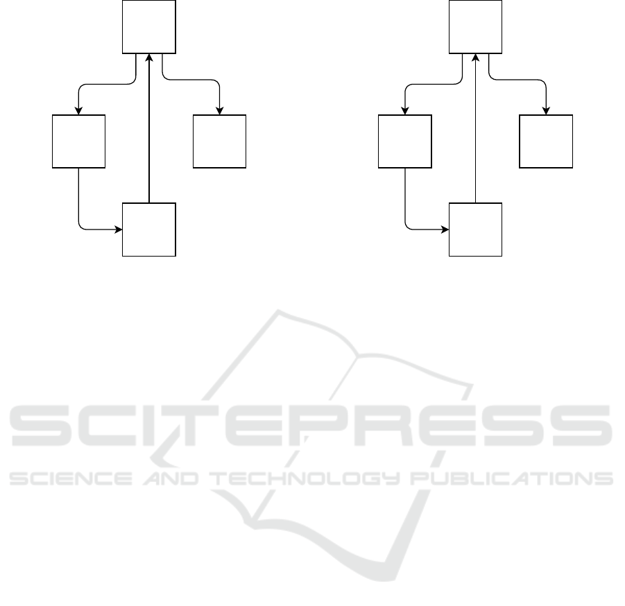
Figure 1: Control ﬂow graph (CFG) of a small program,

visualizing the block-coverage of an example execution.

from the intuition that an input corpus that covers a

more signiﬁcant portion of the program’s code is also

more likely to uncover “buggy” portions of the code.

AFL represents a milestone in the history of fuzzers.

It discovered many bugs in various programs and

paved the way for other successful fuzzers that work

around the same idea. AFL is not maintained any-

more; AFL++ (Fioraldi et al., 2020) is a community-

driven fork of AFL that incorporates state-of-the-art

fuzzing research.

2.3 Coverage Metrics

Many metrics can be used to measure the coverage of

the program code; the key idea behind these metrics is

to recognize different program behaviors. This plays

a key role in coverage-guided fuzzing, as it allows to

recognize which inputs exercise a different behavior

in the program (w.r.t. the inputs currently in the cor-

pus).

Ideally, it is possible to trace the whole execution

path: when the program gets executed, keep track

of the history of which basic-block are visited and

in which order (for instance, h = [B

,...]).

This way, two program executions with different ex-

ecution paths are considered to exercise the program

in a different way. This path-coverage metric allows

to distinguish different program behaviors with very

high sensitivity, but cannot be used in practice: us-

ing this coverage metric in a real-world fuzzer would

make the input corpus grow very large and very fast

(a lot of inputs will be judged interesting and main-

tained because they generate a different execution

path than the ones already seen). On the other ex-

treme, we have block-coverage (Figure 1), a cover-

B3 B2

e1: 3 hits

e2: 3 hits

e3: 1 hits

e4: 3 hits

Figure 2: Control ﬂow graph (CFG) of a small program,

visualizing the edge-coverage of an example execution.

age metric that, for each execution of the program,

counts how many times a certain basic-block is vis-

ited (hit): the output generated by this metric is a map

m = [B

→ c

,...,B

→ c

] where B

is the

i-th block, and c

is the number of times the i-th block

was visited during this program execution.

A trade-off between execution path-coverage and

block-coverage is the edge-coverage (Figure 2); for

a given execution of the program, it keeps track of

the number of hits of a certain edge (edges are the

transitions between basic blocks – in the control ﬂow

graph of the program they are represented as arrows).

The output generated by this metric is a map m =

→ c

,...,e

→ c

] where e

is the i-th

edge, and c

is the number of times the i-th edge was

hit during this program execution. Edge-coverage is

strictly more sensitive than block-coverage, meaning

that: if two program executions have the same edge-

coverage, that implies that they also have the same

block-coverage, but the opposite is not true.

There are many more types of code-coverage

(Wang et al., 2019a), but edge-coverage and block-

coverage are the most popular among state-of-the-art

fuzzers. AFL (and AFL++) use edge-coverage; we

also use edge-coverage within Rainfuzz, both for de-

ciding whether to keep a mutated input in the input-

corpus and to evaluate the effectiveness of a mutation.

3 PROBLEM FORMALIZATION

During fuzzing, the fuzzing engine makes several de-

cisions on the input to be fed to the PUT. For instance,

which input seed should be mutated, and where and

Rainfuzz: Reinforcement-Learning Driven Heat-Maps for Boosting Coverage-Guided Fuzzing

how to perform the mutation. State-of-the-art fuzzers’

engines mostly employ random choices: they pick a

random seed from the pool of interesting seeds, and

they perform ﬁxed and random mutations in a ran-

dom portion of the input seed. In this work, we fo-

cus on the choice of where to apply the mutation, and

we formalize the problem as a reinforcement learn-

ing problem. From the point of view of the RL agent,

inputs to be mutated correspond to states; an action

corresponds to choosing a position within the input

and performing a set of mutations using that position

as an offset; the reward corresponds to a numerical

evaluation of the effectiveness of the mutations.

To better understand the rest of this work, we sum-

marize the main concepts of reinforcement learning

(Section 3.1), with a particular focus on the Proximal

Policy Optimization (PPO) technique (Section 3.2)

used by Rainfuzz.

3.1 Reinforcement Learning

Reinforcement learning is a branch of machine learn-

ing. It studies the problem of an agent interacting with

an environment whose objective is to take actions to

maximize their reward over time.

The environment state S

is the environment’s in-

ternal representation that it uses to produce the next

reward and observation. The reinforcement learning

problem is usually modeled as a Markov Decision

Process (MDP), which requires that the state of the

environment is fully observable by the agent (obser-

vation = S

), and that S

is all that the environment

needs to know in order to deﬁne what are the next

state and reward when the agent takes an action (inde-

pendently from the history of previous states, actions,

rewards). More formally:

MDP = hS,A,P,R,γ,µi

• S is a set of states.

• A is a set of actions.

• P is a state transition probability matrix (|S|∗|A|×

|S|), where each element p

s,s

is the probability to

go from state s to s

when taking action a.

• R is a reward function: R(s,a) =“average reward

when taking action a in state s”.

• γ is the discount factor (γ ∈ [0, 1]); it is used to

compute the cumulative discounted reward, de-

ﬁned as : V =

∑

∞

t=0

t−1

• µ is a vector of probabilities, where each element

is the probability that the initial state is s.

At each time-step t the environment will be in state

∈ S, the agent will pick an action a

∈ A avail-

able in state s

, the environment will return the reward

= R(s

) and the environment will perform a state

transition from s

to s

t+1

according to the state tran-

sition probability matrix P. The episode ends when

the state is terminal (a state without available actions);

episodes are not required to end: there might be inﬁ-

nite episodes. The agent chooses their actions accord-

ing to a policy π; More formally, π(a|s) is the proba-

bility of taking action a when we are in state s.

3.1.1 Solving the RL Problem

The goal of the agent is to act following a policy that

maximizes its reward. When we have full knowl-

edge about the MDP, we can compute a determinis-

tic optimal policy (which is guaranteed to exist for

all MDPs). When the characteristics of the MDP are

unknown (or the size of the model makes it compu-

tationally unfeasible), the agent must learn the policy

by interacting with the environment directly (model-

free methods). Some model-free methods are Monte

Carlo control, SARSA, Q-Learning and policy gradi-

ents.

3.1.2 Policy Gradient Methods

Policy gradients are a class of model-free methods

that allows using a policy approximation as a function

in the state’s features and improving it as the agent

gathers more information by interacting with the envi-

ronment (Mnih et al., 2016), (Schulman et al., 2015),

(Lillicrap et al., 2016), (Barth-Maron et al., 2018).

These methods are based on the policy gradient theo-

rem, which allows to differentiate the expected cumu-

lative reward w.r.t. the policy parameters; this allows,

for example, to compute the gradient and use it for

stochastic gradient ascent.

3.2 Proximal Policy Optimization

The policy gradient theorem can be used directly to

estimate the gradient of the expected reward and per-

form stochastic gradient ascent. Over time, more ad-

vanced objective functions have been developed to

improve the learning process’s performance.

PPO (Schulman et al., 2017) is a state-of-the-art

family of policy gradient methods. It uses different

objective functions designed to overcome some draw-

backs of previous approaches. The objective function

we use in this work is the clipped surrogate objective,

proposed in the original PPO paper, with the addition

of an entropy term; following its deﬁnition:

CLIP+S

(θ) =

∗min(r

(θ),clip(r

(θ),1 − ε, 1 +ε))+ T ∗ S[π

]]

ICPRAM 2023 - 12th International Conference on Pattern Recognition Applications and Methods

where:

• R

is the reward of episode t.

• r

(θ) =

)

old

)

is the probability ratio.

• S[π

] is the entropy of the modelled policy.

• ε is the clip param (an hyper-parameter).

• T is the temperature (an hyper-parameter).

Let’s give an intuition of the role of each term: keep-

ing in mind that our goal is to make our policy more

likely to take high-reward functions, what we want

to maximize is E[R ∗ π

(a|s)] (where the expectation

is over the possible states). In order to estimate this

expected value, we sample experience by following

the policy itself (on-policy learning). We want to take

into consideration the probability of what action is

taken in order to add stability to the learning process;

to reach this goal, we use a technique called impor-

tance sampling, and the expectation becomes:

∗

)

old

)

] = E

∗ r

(θ)].

PPO uses min(r

(θ),clip(r

(θ),1 − ε,1 + ε)) instead

of using r

(θ) directly: This inhibits the effect of

those update steps that would make the new policy

too far away from the old policy, with the goal to

avoid performing destructive updates that might force

the policy to sub-optimal behaviors: since the policy

being learned is the same used for sampling experi-

ence, once the policy becomes too bad, it is impos-

sible to recover from it. This is why it is important

to proceed with caution and avoid greedily perform-

ing very large update steps. The clip param (ε) is the

hyper-parameter that allows deﬁning how far the new

policy is allowed to be with respect to the old pol-

icy. T ∗ S[π

] is an entropy term used to encourage

more stochastic policies. This allows us to handle the

exploration-exploitation dilemma: the ﬁnal goal is to

obtain greater cumulative rewards when using the pol-

icy we are learning (exploitation), but since the policy

used for sampling is the same used for training, it is

also reasonable to leave some possibility for new be-

haviors to take place (exploration), to learn mecha-

nisms that might lead to even greater rewards. The

temperature (T ) is the hyper-parameter deﬁning how

much low-entropy policies are discouraged.

4 RAINFUZZ

State-of-the-art gray-box fuzzers (like AFL) imple-

ment a genetic algorithm that randomly mutates in-

puts and keeps them in the input corpus (for future

mutation) if they discover new edge-coverage in the

program. Our goal is to use this coverage information

not only to decide whether to keep the mutated input

in the input corpus or not but also to evaluate the ef-

fectiveness of the mutation performed. This feedback

about the mutation should allow learning which muta-

tions are effective and which are not, and should allow

taking more effective mutations in the future. Rein-

forcement learning provides a framework that allows

an agent to learn to perform better by interacting with

the environment, and it is a suitable choice to formal-

ize our problem. We list the steps performed within

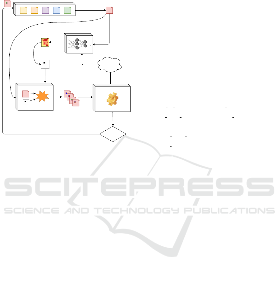
the mutational stage of Rainfuzz, as schematized in

Figure 3: À We pick an input from the queue. Á We

feed the input into the neural-network policy model.

Â The output policy constitutes a heat-map that gives

a probability distribution over the positions within

the current input (higher probability corresponds to a

higher chance that a mutation in that position is effec-

tive). Ã We sample from the probability distribution

given by the heat-map, to retrieve a speciﬁc position

within the input. Ä We feed the input into the mu-

tator, together with the position we sampled. Å The

mutator performs a predeﬁned set of mutations at the

position we just sampled, and we obtain a number of

mutated inputs. Æ We feed the mutated inputs, one

by one, into the executor; the executor runs the PUT

with each one of the mutated inputs while collecting

coverage information. Ç If one or more of the mu-

tated inputs generate new unseen edge-coverage, we

add that mutated input to the queue. È We collect the

coverage information generated by each execution of

the PUT, and we compare it against the coverage gen-

erated by the original un-mutated input; the result of

this comparison is a numerical evaluation of the per-

formance of the mutations at this position: the reward

of the action performed. É We send the reward back

to the policy model, which uses this sampled experi-

ence to train the neural network.

4.1 Learning the Policy: Proximal

Policy Optimization (PPO)

A policy is a mathematical function that, given a

state, returns a probability distribution over the ac-

tions available in that state. Our goal is to improve

the policy over time so that it starts privileging high-

reward actions (which, in our case, corresponds to

performing better mutations). To carry out this learn-

ing task, we decide to use a Policy Gradient method:

Proximal Policy Optimization (PPO).

Rainfuzz: Reinforcement-Learning Driven Heat-Maps for Boosting Coverage-Guided Fuzzing

Input queue

Policy model

Current input

Heatmap

Position to

mutate

Mutator

Mutated Inputs

Executor

New

coverage?

Reward

function

Figure 3: High-level overview of the steps involved in the

fuzzing process of Rainfuzz.

4.1.1 Model of the Policy

PPO provides a method to perform learning steps over

a policy model. The model we choose for the policy

is a Feed Forward Neural Network (FFNN); the in-

put of the NN is the current state of the RL agent (an

array of bytes constituting the input to be mutated);

the output of the NN is a probability distribution over

the actions available in the current state (a heat-map

indicating which byte offsets are more interesting for

applying mutations). To make sure that the sum of

the output probabilities is 1 we use softmax as the ac-

tivation function of the output layer. Moreover, we do

not allow the input to be larger than a ﬁxed number of

bytes, and we force all the mutations to be within the

allowed size. This can happen, for instance, if the po-

sition of the mutation is the last byte and we want to

perform a multibyte mutation (e.g., MAX INT). In such

a case, we simply perform the mutation and discard

the overﬂowing bytes.

4.1.2 Learning Algorithm

To improve the performance of the policy model, we

perform gradient ascent as deﬁned in Section 3.2. We

perform a single update step by using a mini-batch of

sampled experience:

1. We put each sampled experience < s

> into

a memory buffer;

2. If the memory is full (number of sampled expe-

riences = M, mini-batch size), then we perform a

learning step: we estimate L

CLIP+S

by using the

available experience, we differentiate it with re-

spect to the model parameters, and then we apply

the gradients to the parameters;

3. Each time we perform a learning step, we clear

the memory.

4.2 Mutations

As anticipated (in Section 3), an action corresponds

to performing a set of mutations at a given position

within the input. We perform the following actions at

position pos:

• assign random byte

• add to {byte, dbyte, qbyte} {le, be}

• sub from {byte, dbyte, qbyte} {le, be}

• interesting {byte, dbyte, qbyte} {le, be}

• clone piece {overwrite, insert}

• piece insert

• delete block

4.3 Reward Functions

The last step of our learning model is to quantify the

effectiveness of the last action. To do so, we consider

the difference between the coverage of the original

input (c

orig

, an array where the i − th element con-

tains the hit-count for the i − th edge) and the cover-

age of the mutated inputs (C

new

, an array containing

the edge-coverage of the various mutated inputs gen-

erated by the last action). The general principle we

follow is that when the coverage of one or more of

the mutated inputs hits new edges (or has more hits

on already discovered edges), then the reward should

be positive. We experiment with three different ways

of quantifying the effectiveness of the mutations. We

report the reward function R1 in Algorithm 1, R2 in

Algorithm 2 and R3 in Algorithm 3.

5 EXPERIMENT EVALUATION

The goal of our experimental evaluation is to evaluate

several aspects of Rainfuzz and its approach, answer-

ing the following research questions:

• RQ1: Does Rainfuzz’s policy outperform the ran-

dom policy?

• RQ2: Which amount of randomness in the ac-

tion taken is ideal for ﬁnding the most edges over

time?

ICPRAM 2023 - 12th International Conference on Pattern Recognition Applications and Methods

1 i n p u t : c

orig

, C

new

2 o u t p u t : reward

4 d i f f s = [ ]

5 f o r c

i n C

new

6 d i f f = 0

7 f o r k i n [1,2,..., num edges] :

8 i f c

[k] > c

orig

[k] :

9 d i f f += c

[k] − c

orig

[k]

10 d i f f s . a pp en d ( d i f f )

11 r e t u r n a v e r a g e ( d i f f s )

Algorithm 1: Pseudocode of reward function R1.

1 i n p u t : c

orig

, C

new

2 o u t p u t : reward

4 t o t s = [ ]

5 f o r c

i n C

new

6 t o t = 0

7 f o r k i n [1,2,..., num edges] :

8 i f c

[k] > c

orig

[k] :

9 t o t += 1

10 t o t s . a pp en d ( t o t )

11 r e t u r n a v e r a g e ( t o t s )

Algorithm 2: Pseudocode of reward function R2.

1 i n p u t : c

orig

, C

new

2 o u t p u t : reward

4 t o t s = [ ]

5 f o r c

i n C

new

6 t o t = 0

7 f o r k i n [1,2,..., num edges] :

8 i f c

orig

[k] == 0 and c

[k] > 0 :

9 t o t += 1

10 t o t s . a pp en d ( t o t )

11 r e t u r n max ( t o t s )

Algorithm 3: Pseudocode of reward function R3.

• RQ3: Which Reward Function among the ones

we designed performs best?

• RQ4: What is the overhead introduced for gen-

erating mutations following Rainfuzz’s reinforce-

ment learning policy?

• RQ5: How does Rainfuzz perform with respect to

AFL++?

• RQ6: Can the union of AFL++ and Rainfuzz

(running in a collaborative fuzzing setting) out-

perform two AFL++ instances running in paral-

lel?

• RQ7: Is the conﬁguration of Rainfuzz we tuned

against libjpeg-turbo still effective if the PUT

changes?

Throughout our experiments, we use libjpeg-turbo

as a PUT, a binary taken from FuzzBench, a fuzzing

benchmarking framework developed by Google to

unify fuzzing evaluation. We use a different binary in

RQ7 to conﬁrm the results obtained. We tune the pol-

icy model by going through a hyper-parameter tuning

phase; in this phase, we run experiments where the

reinforcement learning policy and the random policy

co-live; we use the difference between the average re-

ward generated by the reinforcement learning policy

and the one generated by the random policy as a met-

ric to decide which conﬁguration is best. We report

the best-performing conﬁguration among the ones we

tested.

• Activation function for the intermediate layers of

the NN: tanh

• Number of intermediate layers for the NN: 1

• Number of neurons for each intermediate layer of

the NN: 128

• Learning rate for the stochastic gradient ascent

update: 0.0001

• Mini-batch size: 50

• Clip hyper-parameter of the clipped surrogate loss

function: 0.5

• Temperature hyper-parameter of the entropy term

in the loss function: 3.0

We also decide to introduce an amount of actions to

be taken randomly; in RQ2, we discover that 75% is

the percentage that works best while, in RQ3, we ﬁnd

that the best-performing reward function is R1. The

resulting conﬁguration is what we call a tuned version

of Rainfuzz.

RQ1: Does Rainfuzz’s Policy Outperform the

Random Policy? First, we run three 24H long ex-

periments for each reward function we designed. We

discover that for all three reward functions, the re-

inforcement learning policy always outperforms the

random policy in terms of average reward. We re-

port the plot of the average-reward signals for R1

as a sample in Figure 4. We are also interested in

assessing the effectiveness of Rainfuzz in terms of

edge-coverage over time (this is the ultimate metric

we use to determine the effectiveness of two fuzzing

approaches). We run three 24H experiments using

the tuned Rainfuzz, and three 24H experiments using

an equivalent fuzzer that uses the random policy; we

plot the resulting average edge-coverage in Figure 5.

Rainfuzz: Reinforcement-Learning Driven Heat-Maps for Boosting Coverage-Guided Fuzzing

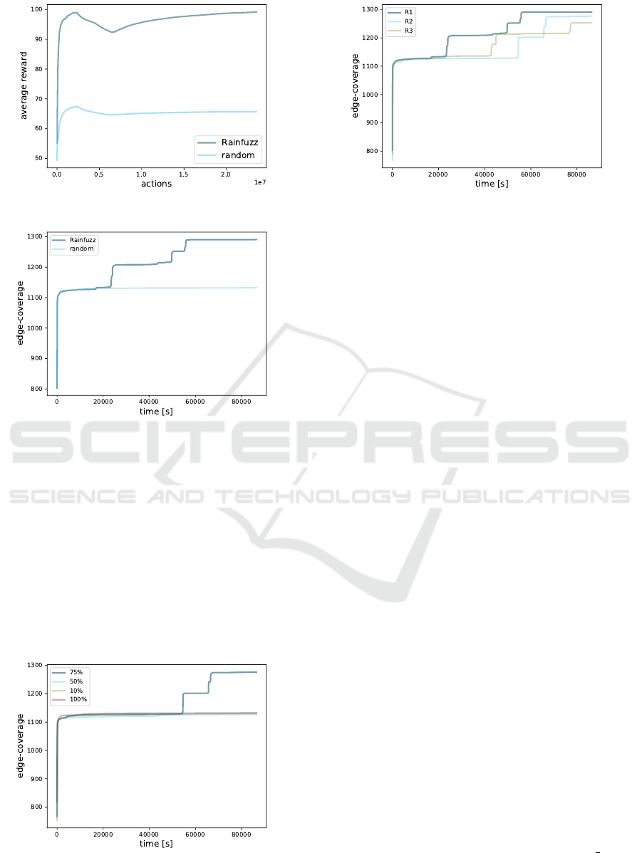
Figure 4: Average rewards generated by R1.

Figure 5: Average edge-coverage generated by Rainfuzz

and by the random policy.

As we can see, the reinforcement learning policy out-

performs the random policy by generating an average

edge-coverage of 1277 against 1133.

RQ2: Which Amount of Randomness in the Ac-

tion Taken Is Ideal for Finding the Most Edges

over Time? We run three 24H long experiments for

each amount of randomness, using R2 as a reward

function. We plot the average edge-coverage in Fig-

ure 6. As we observe, 75% randomness outperforms

the other conﬁgurations by reaching an average edge-

Figure 6: Average edge-coverage generated by each amount

of randomness.

Figure 7: Average edge-coverage generated by each reward

function.

coverage of 1277 (against 1130 for 10%, 1120 for

25% and 1133 for 100%).

RQ3: Which Reward Function Among the Ones

We Designed Performs Best? We run three 24H

long experiments for each reward function we de-

signed and we plot the average edge-coverage in Fig-

ure 7. As we observe, R1 outperforms the other con-

ﬁgurations by reaching an average edge-coverage of

1291 (against 1277 for R2 and 1254 for R3).

RQ4: What Is the Overhead Introduced for

Generating Mutations Following Rainfuzz’s Rein-

forcement Learning Policy? We measure the num-

ber of times the fuzzer executes the PUT per unit of

time. For the random policy we observe an execu-

tion speed of 10624 execs/sec , for Rainfuzz (75%

randomness) we observe 5541 exec/sec, while for a

completely reinforcement learning policy (0% ran-

domness) we observe 2255 exec/sec. As we can see,

when following the reinforcement learning policy, we

execute the PUT at a speed 4,71 lower w.r.t. a com-

pletely random policy: this is the cost introduced by

the need of querying the policy model and training

it. The tuned version of Rainfuzz has an execution

speed that is 1,92 times lower than the random policy,

but our experimental evaluation (RQ1) shows that the

quality of the actions picked compensates the over-

head of choosing them.

RQ5: How Does Rainfuzz Perform with Respect

to AFL++? We want to compare Rainfuzz against

a real-world fuzzer (AFL++). Rainfuzz needs to re-

strict the size of the inputs generated when perform-

ing mutations because they need to ﬁt into the neu-

ral network maximum size. In order to understand

the impact of this restriction, we build aﬂpp mod, a

version of AFL++ that restricts the size of inputs just

like Rainfuzz. We run three 24H long experiments

ICPRAM 2023 - 12th International Conference on Pattern Recognition Applications and Methods

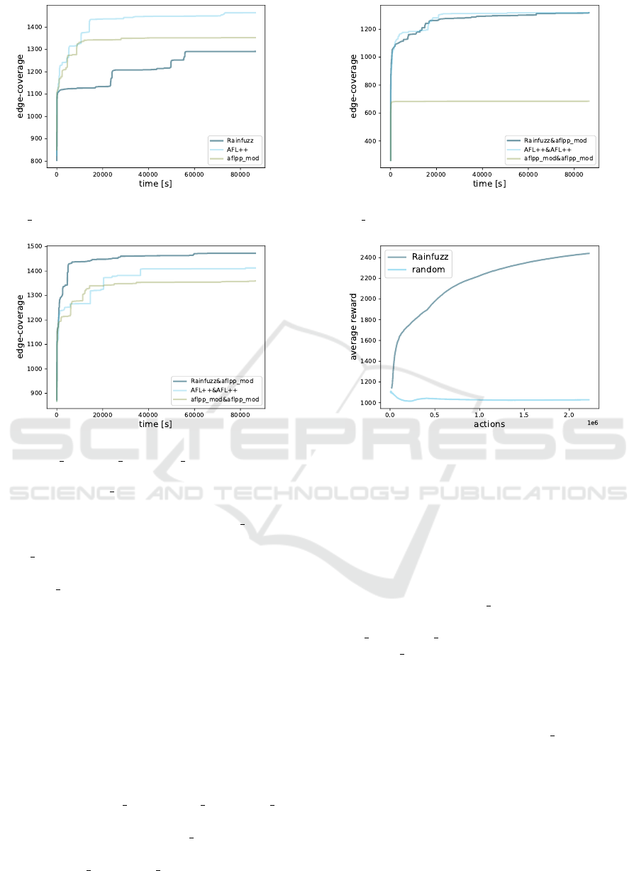
Figure 8: Average edge-coverage generated by Rainfuzz,

aﬂpp mod, AFL++.

Figure 9: Average edge-coverage generated by Rain-

fuzz&aﬂpp mod, aﬂpp mod&aﬂpp mod, AFL++&AFL++

for Rainfuzz, aﬂpp mod and AFL++; we plot the av-

erage edge-coverage in Figure 8. AFL++ generates

an average edge-coverage of 1465, aﬂpp mod 1352

and Rainfuzz 1291. The fact that AFL++ outperforms

aﬂpp mod shows the negative impact of restricting in-

put size. Rainfuzz is outperformed by both AFL++

and aﬂpp mod, but we ﬁnd a more interesting result

in RQ6.

RQ6: Can the Union of AFL++ and Rainfuzz

(Running in a Collaborative Fuzzing Setting)

Outperform Two AFL++ Instances Running in

Parallel?. Collaborative fuzzing is a technique that

consists in running instances of different fuzzers in

parallel; this approach is often capable of exploit-

ing the strengths of different fuzzing approaches

uler et al., 2020). We refer to a setting where an

instance of a fuzzer F1 is ruan in parallel with F2

with F1&F2. We run three 24H long experiments

for Rainfuzz&aﬂpp

mod, aﬂpp mod&aﬂpp mod,

AFL++&AFL++; we plot the average edge-coverage

in Figure 9. Rainfuzz&aﬂpp mod generates an

average edge-coverage of 1473, AFL++&AFL++

1414 and aﬂpp mod&aﬂpp mod 1359.

Figure 10: Average edge-coverage generated by Rainfuzz,

aﬂpp mod, AFL++.

Figure 11: Average reward generated by Rainfuzz, using

file as PUT.

RQ7: Is the Conﬁguration of Rainfuzz We

Tuned Against Libjpeg-Turbo Still Effective

if the PUT Changes?. We are interested in ﬁnd-

ing out if the tuning phase we did is robust, and

can still be effective if the PUT changes; we re-

peat the same set of experiments we ran for RQ6

but using file as PUT, Figure 10 shows the

results. Rainfuzz&aﬂpp mod generates an aver-

age edge-coverage of 1319, AFL++&AFL++ 1317,

aﬂpp mod&aﬂpp mod 685. As we can observe, Rain-

fuzz&aﬂpp mod still outperforms the other two con-

ﬁgurations, but just by a very small amount.

We are also interested in visualizing the effective-

ness of the reinforcement learning policy over the ran-

dom policy. We take the rewards generated by the

Rainfuzz instance of Rainfuzz&aﬂpp mod. We plot

them in Figure 11.

5.1 Threats to Validity

Edge-coverage over time is a metric that is subject

to a discreet amount of variance, and results may

vary a lot due to random chance. For this reason,

we repeated our experiment three times, and we ana-

lyzed the average edge-coverage observed to draw our

Rainfuzz: Reinforcement-Learning Driven Heat-Maps for Boosting Coverage-Guided Fuzzing

conclusions. To deﬁnitely conﬁrm the results of our

work, it’s probably necessary to repeat experiments

more than three times. Moreover, we analyzed the

robustness of the tuned version of Rainfuzz in RQ7,

by observing how Rainfuzz performs against a differ-

ent PUT then jibjpeg-turbo: file. To conﬁrm the

robustness of Rainfuzz it is probably necessary to ex-

periment against a much larger variety of PUTs.

6 RELATED WORKS

Previous attempts tried to use different machine learn-

ing techniques to build heat-maps. In (Rajpal et al.,

2017) the authors experiment with neural network

models capable of predicting heat-maps given an in-

put. Data on the effectiveness of mutations is col-

lected by running a standard gray-box fuzzer (AFL),

and then the neural network is trained using that data,

in a supervised learning setting. The model is then

used to predict what bytes are useful to mutate, and

mutations that don’t stress those bytes are vetoed. In

(She et al., 2019) a neural network model is used

to predict the resulting edge coverage given the in-

put. An adversarial machine learning technique is

then used, to detect the input byte with the highest

gradient associated with it. This is equivalent to detect

the byte that, if mutated, has the highest probability to

cause a change in the output coverage predicted by the

model; if the model is accurate enough, this change

should also be reﬂected in the coverage of the actual

program. This byte is then used as an offset to per-

form a number of mutations. Both these approaches

have the drawback that they must be preceded by a

phase where data is collected and used for training a

model. As the fuzzing process goes on, new program

behaviours are discovered, and the model gets quickly

outdated; since this approaches are based on the effec-

tiveness of the model, a new training phase needs to

be taken in order to update the model. This alterna-

tion between training and fuzzing phases introduces

signiﬁcant overhead.

Also reinforcement learning has been applied to

fuzzing. In (B

ottinger et al., 2018) the authors explore

the possibility of making mutations more efﬁcient by

modelling the fuzzing process as a full reinforcement

learning problem:

• inputs are the states of the MDP.

• an action corresponds to randomly select a sub-

string within the input, and to perform a single

mutation on such a sub-string. The mutation is

chosen accross several available mutations (e.g.,

Delete, Shuffle, Random bit-flips, etc.).

• They experiment with two types of reward: Dis-

covered Blocks and Execution time.

The technique used to solve the reinforcement learn-

ing problem is deep Q-learning: the deep Q-network

observes a portion of the input i (the sub-string s

and estimates the value function Q(s

,a), for each ac-

tion a; they use an ε − greedy policy to choose the

next action to take. Finally, the experimental evalu-

ation compares the approach against a baseline cre-

ated using the random policy. The metric they use

is the cumulative reward generated by the two poli-

cies, proving that the reinforcement learning policy

chooses higher reward functions. However, this eval-

uation has a limitation. The metric used during ex-

perimental evaluation shows an interesting theoreti-

cal result, but does not provide evidence of the ef-

fectiveness of the approach in a real-world scenario:

overheads introduced by the reinforcement learning

approach might defeat the purpose; edge-coverage

over time is the right metric to use if we want to

test the effectiveness of a fuzzer in a real-world sce-

nario. For completeness we cite (Zhang et al., 2020),

another approach that uses reinforcement learning in

fuzzing. The formalization of the problem is very

similar to the one used in (B

ottinger et al., 2018). The

main difference is related to the algorithm they use for

solving the reinforcement learning problem, an actor-

critic technique: Deep Deterministic Policy Gradient.

Their experimental evaluation explores many hyper-

parameters combinations, but ultimately uses a met-

ric similar to the one used in (B

ottinger et al., 2018),

proving a result that is theoretically interesting, but

with no direct impact on real-world fuzzing.

7 FUTURE WORKS

A key role in Rainfuzz is played by the reward func-

tion, which evaluates the effectiveness of the muta-

tions taken in a given position within the input. In

our implementation, we experiment with three reward

functions, but there is space for more approaches. We

propose the creation of a reward function that weights

edges differently based on their rarity: a mutation that

allows increasing the hit count on edges that are not

seen very often should be rewarded more than a mu-

tation that allows increasing the hit count on edges

that are already stressed very frequently by the cur-

rent input-corpus. This idea of taking into account the

rarity of edges was already explored in the context of

seed scheduling (B

ohme et al., 2016) with great re-

sults; we believe that shifting this concept in the con-

text of rewarding mutations is very promising.

The NN architecture we use in Rainfuzz has a

ICPRAM 2023 - 12th International Conference on Pattern Recognition Applications and Methods

ﬁxed input size, forcing us to restrict the size of mu-

tated inputs. There is space for experimentation to

overcome this issue by using different NN architec-

tures. Probably recurrent NNs are a suitable choice,

but it faces the challenge of modeling a variable-

length policy.

An important component of Rainfuzz is the set of

position-speciﬁc mutations (Section 4.2) correspond-

ing to a single action. The mutations we use are

inspired by random-position mutations that are used

within AFL++; it might be interesting to experiment

with different sets of position-speciﬁc mutations and

study how they inﬂuence the performance of fuzzing

based on the input format of the PUT.

8 CONCLUSIONS

In this paper, we propose an innovative fuzzing ap-

proach that builds heat-maps using reinforcement

learning, aiding the mutation strategy and overcom-

ing the issue of alternating training phases to fuzzing

phases. We implemented our approach by means of

Rainfuzz, and we tuned it by trying different con-

ﬁgurations (RQ2, RQ3). We tested the validity of

our approach (RQ1) by comparing Rainfuzz against

an equivalent fuzzer that uses a fully random policy,

showing that Rainfuzz performs better both in terms

of average reward per action and in terms of edge-

coverage. We tested Rainfuzz against a state-of-the-

art fuzzer (AFL++), with poor results (RQ5); but we

showed that Rainfuzz and AFL++ running in a col-

laborative fuzzing setting obtain the best performance

(RQ6). We conﬁrmed the robustness of Rainfuzz by

showing that the previous results still apply if the PUT

changes (RQ7). Finally, we concluded by providing

some ideas to extend and improve the approach we

proposed.

ACKNOWLEDGEMENTS

Lorenzo Binosi acknowledges support from TIM

S.p.A. through the PhD scholarship.

REFERENCES

Barth-Maron, G., Hoffman, M. W., Budden, D., Dabney,

W., Horgan, D., TB, D., Muldal, A., Heess, N., and

Lillicrap, T. P. (2018). Distributed distributional de-

terministic policy gradients. CoRR, abs/1804.08617.

ohme, M., Pham, V., and Roychoudhury, A. (2016).

Coverage-based greybox fuzzing as markov chain. In

Weippl, E. R., Katzenbeisser, S., Kruegel, C., Myers,

A. C., and Halevi, S., editors, Proceedings of the 2016

ACM SIGSAC Conference on Computer and Commu-

nications Security, Vienna, Austria, October 24-28,

2016, pages 1032–1043. ACM.

ottinger, K., Godefroid, P., and Singh, R. (2018). Deep

reinforcement fuzzing. In 2018 IEEE Security and

Privacy Workshops, SP Workshops 2018, San Fran-

cisco, CA, USA, May 24, 2018, pages 116–122. IEEE

Computer Society.

Chen, C., Cui, B., Ma, J., Wu, R., Guo, J., and Liu, W.

(2018). A systematic review of fuzzing techniques.

Comput. Secur., 75:118–137.

Fioraldi, A., Maier, D., Eißfeldt, H., and Heuse, M. (2020).

AFL++ : Combining incremental steps of fuzzing re-

search. In Yarom, Y. and Zennou, S., editors, 14th

USENIX Workshop on Offensive Technologies, WOOT

2020, August 11, 2020. USENIX Association.

Google (2016). HonggFuzz. https://honggfuzz.dev/.

uler, E., G

orz, P., Geretto, E., Jemmett, A.,

Osterlund, S.,

Bos, H., Giuffrida, C., and Holz, T. (2020). Cupid :

Automatic fuzzer selection for collaborative fuzzing.

In ACSAC ’20: Annual Computer Security Applica-

tions Conference, Virtual Event / Austin, TX, USA, 7-

11 December, 2020, pages 360–372. ACM.

Lillicrap, T. P., Hunt, J. J., Pritzel, A., Heess, N., Erez, T.,

Tassa, Y., Silver, D., and Wierstra, D. (2016). Con-

tinuous control with deep reinforcement learning. In

Bengio, Y. and LeCun, Y., editors, 4th International

Conference on Learning Representations, ICLR 2016,

San Juan, Puerto Rico, May 2-4, 2016, Conference

Track Proceedings.

LLVM (2017). libFuzzer. http://llvm.org/docs/LibFuzzer.

html.

Man

es, V. J. M., Han, H., Han, C., Cha, S. K., Egele, M.,

Schwartz, E. J., and Woo, M. (2021). The art, science,

and engineering of fuzzing: A survey. IEEE Trans.

Software Eng., 47(11):2312–2331.

Mnih, V., Badia, A. P., Mirza, M., Graves, A., Lillicrap,

T. P., Harley, T., Silver, D., and Kavukcuoglu, K.

(2016). Asynchronous methods for deep reinforce-

ment learning. CoRR, abs/1602.01783.

Rajpal, M., Blum, W., and Singh, R. (2017). Not all

bytes are equal: Neural byte sieve for fuzzing. CoRR,

abs/1711.04596.

Schulman, J., Levine, S., Moritz, P., Jordan, M. I., and

Abbeel, P. (2015). Trust region policy optimization.

CoRR, abs/1502.05477.

Schulman, J., Wolski, F., Dhariwal, P., Radford, A., and

Klimov, O. (2017). Proximal policy optimization al-

gorithms. CoRR, abs/1707.06347.

She, D., Pei, K., Epstein, D., Yang, J., Ray, B., and Jana,

S. (2019). NEUZZ: efﬁcient fuzzing with neural pro-

gram smoothing. In 2019 IEEE Symposium on Secu-

rity and Privacy, SP 2019, San Francisco, CA, USA,

May 19-23, 2019, pages 803–817. IEEE.

Wang, J., Duan, Y., Song, W., Yin, H., and Song,

C. (2019a). Be sensitive and collaborative: An-

alyzing impact of coverage metrics in greybox

Rainfuzz: Reinforcement-Learning Driven Heat-Maps for Boosting Coverage-Guided Fuzzing

fuzzing. In 22nd International Symposium on Re-

search in Attacks, Intrusions and Defenses, RAID

2019, Chaoyang District, Beijing, China, September

23-25, 2019, pages 1–15. USENIX Association.

Wang, Y., Jia, P., Liu, L., and Liu, J. (2019b). A system-

atic review of fuzzing based on machine learning tech-

niques. CoRR, abs/1908.01262.

Zalewski, M. (2016). AFL: American Fuzzy Lop

- Whitepaper. https://lcamtuf.coredump.cx/aﬂ/

technical details.txt.

Zhang, Z., Cui, B., and Chen, C. (2020). Reinforcement

learning-based fuzzing technology. In Barolli, L.,

Poniszewska-Maranda, A., and Park, H., editors, In-

novative Mobile and Internet Services in Ubiquitous

Computing - Proceedings of the 14th International

Conference on Innovative Mobile and Internet Ser-

vices in Ubiquitous Computing (IMIS-2020), Lodz,

Poland, 1-3 July, 2020, volume 1195 of Advances in

Intelligent Systems and Computing, pages 244–253.

Springer.

ICPRAM 2023 - 12th International Conference on Pattern Recognition Applications and Methods