Multi-Agent Pathﬁnding on Large Maps Using Graph Pruning:

This Way or That Way?

Svancara

1 a

, Philipp Obermeier

2 b

, Matej Hus

, Roman Bart

1 c

and Torsten Schaub

2 d

Charles University, Prague, Czech Republic

University of Potsdam and Potassco Solutions, Potsdam, Germany

Keywords:

Multi-Agent Pathﬁnding, Answer Set Programming, Subgraph, Shortest Path.

Abstract:

Multi-agent pathﬁnding is the task of navigating a set of agents in a shared environment from their start

locations to their desired goal locations without collisions. Solving this problem optimally is a hard task and

various algorithms have been devised. The algorithms can generally be split into two categories, search- and

reduction-based ones. It is known that reduction-based algorithms struggle with large instances in terms of

the size of the environment. A recent study tried to mitigate this drawback by pruning some vertices of the

environment map. The pruning is done based on the vicinity to a shortest path of an agent. In this paper, we

study the effect of choosing such shortest paths. We provide several approaches to choosing the paths and we

perform an experimental study to see the effect on the runtime.

1 INTRODUCTION

We study the problem of Multi-agent pathﬁnding

(MAPF). The task is to navigate a set of agents in

a shared environment (map) from starting locations

to the desired goal locations such that there are no

collisions (Silver, 2005). This problem has numerous

practical applications in robotics, logistics, digital en-

tertainment, automatic warehousing and more, and it

has attracted signiﬁcant focus from various research

communities in recent years (Li et al., 2020; Surynek,

2019; Nguyen et al., 2017; Gebser et al., 2018b).

Optimal MAPF solvers can generally be split into

two categories, search- and reduction-based ones.

The former search over possible locations or conﬂicts

among agents, while the latter reduce the problem

to other formalisms, such as Answer Set Program-

ming (ASP) (Gebser et al., 2018a). While it is not

always the case, it is generally established that each

of the approaches dominates on different types of in-

stances (G

omez et al., 2021; Svancara and Bart

ak,

2019). The search-based solvers are easily able to

ﬁnd solutions on large sparsely populated maps while

having trouble dealing with small densely populated

https://orcid.org/0000-0002-6275-6773

https://orcid.org/0000-0001-6346-4855

https://orcid.org/0000-0002-6717-8175

https://orcid.org/0000-0002-7456-041X

maps. On the other hand, the reduction-based solvers

are able to deal with the small densely populated maps

but are unable to ﬁnd a solution for large maps even

with a small number of agents.

Since reduction-based solvers have trouble solv-

ing large instances, a recent study (Hus

ar et al., 2022)

proposed techniques to remove vertices from the map

that are most likely not needed to solve the instance.

The pruning is done based on a random shortest path

for each agent. Only vertices around the selected path

are considered and other vertices are removed, creat-

ing a much simpler problem. In this paper, we extend

the original study by examining the behavior of the

technique by using more than just one shortest path

for each agent. First, we describe the four pruning

strategies from the original study, and then we intro-

duce four new ones to select paths for each agent.

2 DEFINITIONS

A MAPF instance M is a pair (G,A), where G is a

graph G = (V, E) and A is a set of agents. An agent

∈ A is a pair a

= (s

, g

), where s

∈ V is the start

location and g

∈ V is the goal location of agent a

Our task is to ﬁnd a valid plan π

for each agent

∈ A being a valid path from s

to g

. We use

(t) = v to denote that agent a

is located at vertex v

Švancara, J., Obermeier, P., Husár, M., Barták, R. and Schaub, T.

Multi-Agent Pathﬁnding on Large Maps Using Graph Pruning: This Way or That Way?.

DOI: 10.5220/0011625100003393

In Proceedings of the 15th International Conference on Agents and Artiﬁcial Intelligence (ICAART 2023) - Volume 1, pages 199-206

ISBN: 978-989-758-623-1; ISSN: 2184-433X

 2023 by SCITEPRESS – Science and Technology Publications, Lda. Under CC license (CC BY-NC-ND 4.0)

199

at timestep t. Time is discrete and at each timestep, an

agent can either wait at its current location or move to

a neighboring location. Furthermore, we require that

each pair of plans π

and π

, i 6= j is collision-free.

Based on MAPF terminology (Stern et al., 2019),

there are ﬁve types of collisions. Here, we forbid

edge, vertex, and swap conﬂicts while allowing follow

and cycle conﬂicts since the two latter prevent agents

from occupying the same location. Note, however,

that all of our methods work in any setting.

We are interested in makespan optimal solutions.

Makespan (or horizon) refers to the length of a plan.

A plan ends once all of the agents are at the goal lo-

cation at the same time. This means that the length of

the plan |π

| is the same for all of the agents. Another

common cost function is sum of costs (Sharon et al.,

2011). Note that ﬁnding an optimal solution for either

of the cost functions is an NP-hard problem (Ratner

and Warmuth, 1990; Yu and LaValle, 2013).

3 ASP ENCODING

We use an ASP encoding

for MAPF due to (Gebser

et al., 2018a). The encoding assumes a grid graph G

and plans agents in parallel within a makespan while

avoiding conﬂicts. Speciﬁcally, the plan’s timesteps

are bound by the makespan H in Line 1. Line 3 gives

the four cardinal directions, used in Line 4 to repre-

sent all transitions on the grid with its x,y-coordinates

stated by predicate position/1. Possible movement

actions, at most one per agent and timestep, are gen-

erated by Line 8. Related preconditions and posi-

tional changes are described in Lines 10-12: The posi-

tions of all agents are described by position(R,C,T

) stating that agent R is at x,y-coordinates C at time

T. For an agent R sitting idle at time T, the frame ax-

iom in Lines 14-15 propagates its unchanged position.

Swapping conﬂicts are prevented by Lines 17-19, and

both edge and vertex conﬂicts by Line 21.

1 time ( 1. . h ori zon ) .

3 dire cti on (( X,Y ) ) :- X = - 1..1 , Y = -1..1

, | X + Y |=1.

4 nex tto (( X,Y ) , ( D X,DY ) ,(X ’ ,Y ’) ) :-

5 dir ect ion (( DX, DY )), pos iti on ((

X, Y ) ) , p osi tio n (( X ’ ,Y ’) ),

6 ( X,Y ) =( X ’ - DX,Y ’-DY ) , ( X ’,Y ’) =( X +

DX,Y + DY ) .

8 { m ov e ( R,D,T ) : d ire cti on ( D ) } 1 : -

isR obo t ( R ) , time ( T).

10 posit io n ( R,C, T ) :-

https://github.com/potassco/asprilo-encodings/blob/

master/m/action-M.lp

11 m ove ( R, D , T ) , pos i ti o n ( R,C ’,T -1) ,

nex t to (C ’ ,D , C ) .

12 :- mo v e ( R,D,T ) , pos it i on ( R,C ,T -1) ,

no t ne xtt o ( C ,D, _ ) .

14 po si t io n ( R,C, T ) :-

15 pos it i on ( R,C,T -1) , n ot move (

R,_, T ) , i s Ro b ot ( R ) , t i m e ( T ).

17 mov eto (C ’ ,C,T ) : -

18 next to (C ’ , D ,C ) , pos i ti o n ( R,C ’,T

-1 ) , mov e ( R ,D,T ) .

19 :- move t o ( C ’ ,C , T ) , m ove to ( C,C ’,T ) ,

C < C ’.

21 :- { p os i ti on ( R ,C,T ) : isR o bo t ( R ) }

> 1 , po s it i on ( C) , t i me ( T ) .

Listing 1: Action theory for agent movements.

Further, we augment the action theory encoding with

the goal condition in Listing 2 to enforce that every

agent R has reached its goal coordinates C, stated by

goal(R,C), at the time H.

1 :- n ot po s it io n ( R, C, ho ri z o n ) , go a l (

R, C ) .

Listing 2: Goal condition for agents and assigned nodes.

There are two common techniques to speed up

computation. First, using a lower bound for the

makespan. A simple lower bound is to compute for

each agent a

the shortest path from its start loca-

tion s

to its goal location g

. The lower bound for

H is then the longest of these shortest paths. Another

enhancement is to preprocess the variables represent-

ing agent locations. These variables correspond to an

agent being present at some location at a time. How-

ever, for some locations, the speciﬁc agent cannot be

present at the speciﬁc times. Speciﬁcally, for agent

, if vertex v is distance d away from start location

, we know that the agent a

cannot be at vertex v at

times 0, . . . , (d −1). Similarly, if vertex v is distance d

away from goal location g

, agent a

cannot be present

at vertex v at times H − d + 1, . . . , H.

4 THE SUB-GRAPH METHOD

Both of the above improvements maintain complete-

ness and optimality. However, there are situations,

where too many possibilities for an agent’s location

remain, which may overwhelm the underlying solver.

The motivation of (Hus

ar et al., 2022) can be seen in

Figure 1a. The agent is placed on a 4-connected grid

going from one corner to the diagonally opposite cor-

ner. With just one agent and no obstacles, there are



2(N−1)

N−1



possible shortest paths on an N × N grid. As

ICAART 2023 - 15th International Conference on Agents and Artiﬁcial Intelligence

200

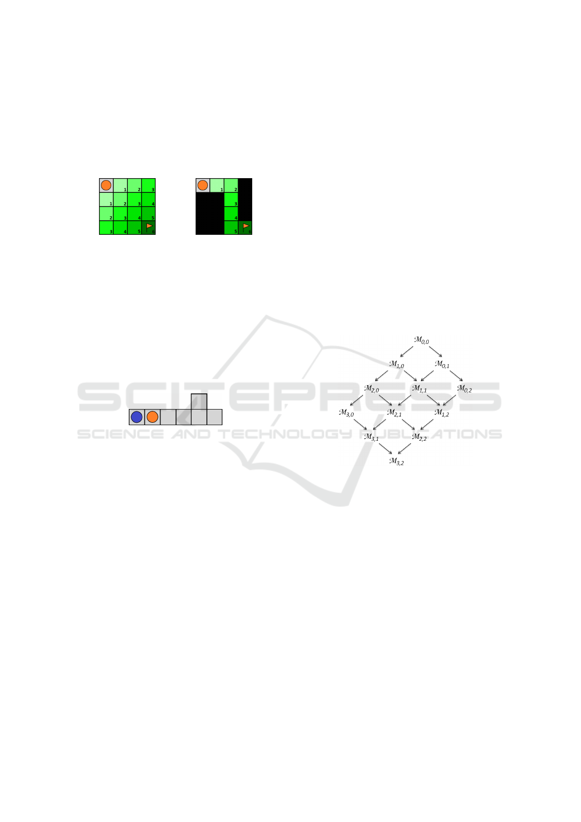
shown in the ﬁgure, preprocessing ﬁnds out at what

timesteps the agent can be located at which vertices.

However, the number of choices is still too large for

the solver. The idea is to pick just one of the shortest

paths and to treat the other vertices as impassable ob-

stacles. So, for these vertices, no variables enter the

solver. This pruning is shown in Figure 1b.

(a)

(b)

Figure 1: An agent moving on a grid map from a corner to

the opposite one. The numbers represent at what timesteps

the agent can reach the given vertex.

Of course, this pruning does not maintain com-

pleteness in general. A simple counterexample is

given in Figure 2. The two agents want to swap their

location (ie. their goal location is identical with the

starting location of the other agent). To do this, the

only solution is for both of them to travel to the right

and use the top vertex to switch their position. To mit-

igate these instances, several strategies are proposed

to change which vertices are pruned.

Figure 2: An instance with two agents that want to swap

their positions.

4.1 Solving Strategies

Let SP

be the set of vertices on a chosen short-

est path for agent a

∈ A (ie. a single shortest path

from s

to g

). The length of the path is |SP

|. The

union of vertices on the shortest paths of all agents is

∈A

. Note that we consider a single short-

est path for each agent. If multiple shortest paths exist

for an agent, one is chosen at random. Given this, the

lower bound on the makespan of an instance (G, A)

is LB

mks

(G, A) = max

∈A

|SP

|. For short, we refer to

such lower bound just by LB.

A k-restricted graph Gres

is a subgraph of G

containing only vertices SP

and vertices at most dis-

tance k away from some vertex in SP

. Since we

always ﬁx SP

, we write for simplicity only Gres

Note that Gres

⊆ Gres

for k ≤ k

We deﬁne a makespan-restricted MAPF instance

as M = (G, A, H). A makespan optimal solution is

found by iteratively increasing the makespan. The

(k,m)-relaxation of M is the makespan-restricted

MAPF instance

k,m

= (Gres

, A, LB +m)

This relaxation considers only Gres

instead of the

whole graph G. We ﬁnd a solution with ex-

tra makespan m – extra over the lower bound on

makespan. Also note that Gres

is constructed such

that LB

mks

(G, A) = LB

mks

(Gres

, A) for any k, there-

fore, we do not need to change the notation of LB.

We build a partial order ≺

relax

over the (k,m)-

relaxations M

k,m

such that

k,m

≺

relax

if k ≤ k

, m ≤ m

and k +m < k

+ m

There is an upper bound on k such that for some

max

we have Gres

max

= G. There is also an upper

bound on the makespan for a given MAPF instance

of O(V

) (Kornhauser et al., 1984). For example, as-

sume that k

max

= 3 and m

max

= 2. Then, Figure 3

depicts the space of possible relaxations induced by

≺

relax

. Note that the partial ordering forms a lattice.

Figure 3: Instance relaxations for k

max

= 3, m

max

= 2.

The generic algorithm to solve MAPF using the

relaxed instances is as follows. First, we build an ini-

tial (k,m)-relaxation and we iteratively change k and

m until the instance is solvable. This corresponds to a

traversal of the lattice formed by the partial ordering

≺

relax

. Note that the shortest path for each agent is

ﬁxed for all of the iterations.

Next, we identify four reasonable traversals.

Baseline Strategy. The classical approach to

solving MAPF makespan optimally can be expressed

in the relaxed instances as follows. We start with an

initial candidate of k

max

(ie. the whole graph G) and

m = 0. If the relaxed instance is unsolvable, only the

additional makespan m is increased to m +1. We shall

refer to this strategy as baseline or B for short.

Proposition 1. If a MAPF instance M has a solution,

baseline strategy ﬁnds an optimal solution.

Makespan-add Strategy. The ﬁrst smarter solu-

tion is to keep only the vertices on the shortest paths

Multi-Agent Pathﬁnding on Large Maps Using Graph Pruning: This Way or That Way?

201

and the immediately adjacent ones. The initial candi-

date is k = 1 and m = 0. Otherwise, the strategy is the

same as the baseline strategy: if the relaxed instance

is unsolvable, we increase m to m + 1 while k is never

changed. We refer to this strategy as makespan-add

or M for short.

Proposition 2. (Hus

ar et al., 2022) The makespan-

add strategy is both suboptimal and incomplete.

On the other hand, in most cases, this simple strat-

egy can ﬁnd a solution, and due to the great reduction

of vertices of the graph, the solution may be found

quickly. We choose to start with k = 1 rather than

k = 0 to increase the probability for a solution to exist

while keeping the number of vertices to a minimum.

Prune-and-Cut Strategy. The previous strategies

either use unnecessary large restricted graph or do not

guarantee to ﬁnd a solution. Strategy prune-and-cut

(P for short) guarantees both completeness and op-

timality. We start with initial candidate k = 0 and

m = 0. In case the relaxed instance is unsolvable,

we cannot be sure if the reason is the restriction on

k or on m. However, since we do not want to over-

estimate m, we ﬁrst need to increase k potentially up

to k

max

. Once a restricted instance M

max

is unsolv-

able, we are sure that m needs to be increased. We

can optimistically assume that the whole Gres

max

not needed and we restrict the graph back to k = 0

producing M

0,m+1

Proposition 3. (Hus

ar et al., 2022) If a MAPF in-

stance M has a solution, prune-and-cut strategy ﬁnds

an optimal solution.

Combined Strategy. The drawback of the prune-

and-cut strategy is that in the case the makespan needs

to be increased, we ﬁrst increase k up to k

max

before

increasing m. To mitigate this problem, we present the

combined strategy (C for short). The initial candidate

is again k = 0 and m = 0. If the relaxed instance is

unsolvable, we increase both k = k + 1 and m = m +

1 at the same time. This way, we save solver calls

because we do not need to explore all of the possible

reductions in the k direction. On the other hand, this

strategy is no longer optimal. Figure 4 with blue agent

choosing the blue path is a counterexample.

Proposition 4. (Hus

ar et al., 2022) If a MAPF in-

stance M has a solution, combined strategy is guar-

anteed to ﬁnd a solution (completeness) but not nec-

essarily an optimal one.

Figure 4: An example instance where the blue agent has

two choices of the shortest path. If the blue path is chosen,

the proposed strategies perform worse.

5 CHOOSING THE SHORTEST

PATHS

The described strategies (except for baseline) may

suffer from a poor choice of the initial shortest path

for each agent. See the example in Figure 4. The blue

agent has two possible shortest paths. If the algorithm

by random chooses the blue path, none of the sophis-

ticated strategies can solve the relaxed instance in the

ﬁrst solver call. Makespan-add would ﬁnd a subop-

timal solution with makespan LB + 2, prune-and-cut

would require to increase k two times to be able to use

the black path, and combined strategy would also ﬁnd

a suboptimal solution with makespan LB + 2.

This issue can be mitigated by including all of the

vertices on all of the possible shortest paths into the

Gres

, however, this goes against the logic of the mo-

tivational example in Figure 1. Hence, we try to iden-

tify approaches to choose more than just one of the

shortest paths to improve the strategies.

Since the choice of the shortest paths acts as a

preprocessing stage, we aim for fast heuristic tech-

niques. For this reason, each agent is treated individ-

ually, without considering the interference with short-

est paths of the other agents. We propose the fol-

lowing four sensible approaches to pick which ver-

tices should be included in the initial restricted graph

Gres

. All of the described strategies, then, work the

same as was described in the previous section.

Single Path. First, we use the same approach as

in the original study (Hus

ar et al., 2022). For each

agent, we choose a single random shortest path. The

restricted graph Gres

is induced by SP

∈A

Recall that SP

are the vertices on the shortest path for

agent a

. We refer to this approach as single-path or

SP for short.

All Paths. The second approach is on the other

end of the spectrum. Instead of just one shortest

path, we consider all vertices on all shortest paths

of a given agent. Formally, we write SP

All

= {v ∈

V | dist(s

, v) + dist(v, g

) = |SP

|} meaning all ver-

tices whose distance from start location plus the dis-

ICAART 2023 - 15th International Conference on Agents and Artiﬁcial Intelligence

202

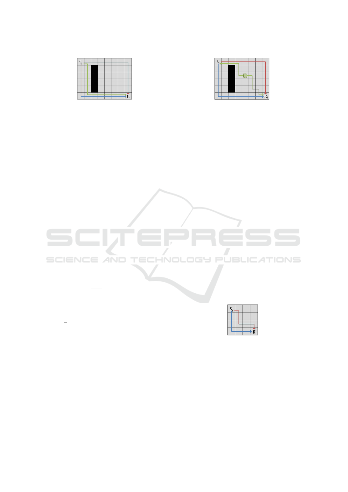
(a) The greedy approach starting at s

chooses an undesir-

able green path due to the fact that it tries to make the path

most divers (to the previously planned blue and red paths)

from the start without the knowledge of the rest of the map.

(b) By choosing a different starting location, the greedy al-

gorithm ﬁnds a better green path than in Figure 5a. In this

example there are multiple possible starting locations, each

equally good. If this happens, one is chosen at random.

Figure 5: An example showing the drawback of ﬁnding the shortest path greedily from the the starting location s

. This issue

can be ﬁxed by choosing different starting vertex. The green path is chosen after red and blue paths.

tance to goal location equals the distance of a short-

est path. The restricted graph Gres

is induced by

All

∈A

All

Note that while there may be many different short-

est paths as discussed in Figure 1, the number of ver-

tices on those paths is much smaller. For the creation

of the restricted graph, we are interested only in the

vertices, the speciﬁc path is decided by the underlying

solver. Finding all of the vertices on all of the shortest

paths can be done by performing a breath-ﬁrst search

from the start and goal of the agent and checking for

the condition in the deﬁnition of SP

All

. We refer to

this approach as all-paths or AP for short.

Random Paths. Instead of considering one or all

possible paths, we aim to pick vertices that are part

of just some subset of all paths. First, we need to

set a number of paths to consider. Note that based

on the given map and the start and goal locations of

each agent, there is a wide variety of the number of

shortest paths. Instead of selecting a magic constant,

we propose to ﬁnd

|SP

All

|SP

shortest paths for agent a

and consider the union of vertices on those. If there is

a unique shortest path, by using the formula we cor-

rectly consider just the one shortest path, while on an

empty N × N grid (such as in Figure 1), we are con-

sidering

paths.

The next proposed approach picks the speciﬁed

number of shortest paths randomly. We do this by

a random walk starting at s

moving only over ver-

tices from SP

All

in the correct direction. We know

the correct direction based on the distance from s

and g

computed by BFS (we need to perform the two

BFS in order to determine SP

All

). The random walk

is biased to prefer vertices that are not yet used for

a given agent. By doing this for all agents we get

Rand

∈A

Rand

. We refer to this approach as

random-paths or RP for short.

Distant Paths. The drawback of random-paths it

that there is no guarantee on the properties of the cho-

sen shortest paths. The idea of using more than one

shortest path is to allow the underlying solver to navi-

gate the agent through a different region of the map to

avoid possible conﬂicts. However, by choosing ran-

dom paths, we may produce paths that share many

vertices or are in close proximity to each other, both

of which are undesirable.

We want to ﬁnd diverse and distant paths. There

is a polynomial-time algorithm to ﬁnd diverse short-

est paths (Hanaka et al., 2021). In this case, diverse

means paths that share the least amount of edges (or

vertices). By using this algorithm, it may be the case

that we ﬁnd paths as shown in Figure 6. On the other

hand, there is also a research dealing with ﬁnding the

most diverse near-shortest paths (H

acker et al., 2021),

in which case the paths are supposed to be the greatest

distance from each other. Note that both studies use

the term distant with different meaning. In our pa-

per, we are using diverse for different paths and dis-

tant for path with distance between them. The down-

side of the the second referred study is that the paths

found are not optimal and also the problem itself is

NP-Hard, which is not a desirable trait for a prepro-

cessing function.

Figure 6: Possible shortest paths from s

to g

found by the

diverse shortest paths algorithm (Hanaka et al., 2021).

Our proposed approach is heuristic. Again, we

build the paths over the vertices from SP

All

, gradu-

ally creating SP

Dist

. At each step, we try to add a new

vertex to the currently build path and if there are mul-

tiple choices, we pick one that maximizes the minimal

distance to all of the vertices currently in SP

Dist

(see

Figure 7 for an example). Since this is just a heuris-

tic, there are examples that make us choose an unde-

sirable path because the approach greedily chose the

next vertex on the path without knowledge of the rest

Multi-Agent Pathﬁnding on Large Maps Using Graph Pruning: This Way or That Way?

203

Figure 7: The gradual building of SP

Dist

from s

to g

a greedy approach. The currently build green path has a

choice. Moving downward will be chosen since it maxi-

mizes the distance to the already chosen paths.

of the map. Such example can be seen in Figure 5a.

To mitigate this, we start to build the path from a dif-

ferent vertex from the set SP

All

rather than from s

The ﬁrst path is build the same as SP

, for the latter

paths, we choose a vertex v such that it maximizes

the minimal distance to all of the vertices currently in

Dist

. This way we need to build the path both from

v to s

and from v to g

. Using this approach we ﬁnd

a much more desirable path for the example in Fig-

ure 5a with the result shown in Figure 5b. We refer to

this approach as distant-paths or DP for short.

6 EXPERIMENTAL EVALUATION

To test and compare the proposed strategies in com-

bination with approaches to creating the restricted

graph, we set up experiments. The full implemen-

tation and results are available at https://github.com/

potassco/mapf-subgraph-system. For the ASP-based

solver, we used the grounding-and-solving system

clingo (Gebser et al., 2019; Kaminski et al., 2020)

version 5.5.2. We ran the experiments on an Intel

Xeon E5-2650v4 under Debian GNU/Linux 9, with

each instance limited to 300s processing time and 28

GB of memory.

The instances used in our experiments are based

on commonly used benchmark instances available on-

line (Stern et al., 2019). We chose different sizes of

maps – small (32 by 32), medium (64 by 64), and

large (128 by 128) and different structures of the im-

passable obstacles in the map with the following types

– empty, maze, random, and room.

For the placement of the agents (called scenarios),

we used the available scenarios. Furthermore, we cre-

ated new scenarios for each map such that the distance

from start to goal of each agent is similar and the paths

of the agents need to cross more often. We did this be-

cause the makespan optimal solution for the random

scenarios rarely differs from the lower bound. The

behavior of the strategies may be gravely affected by

many conﬂicts and the need to increase the makespan.

The intended way to use the benchmark set is to

create an instance of MAPF from a map and a num-

ber of agents from a scenario. If the instance is solved

in the given time limit, an additional agent from the

same scenario is added and thus a new MAPF in-

stance is produced. Once the instance cannot be

solved in the time limit, it is reasoned that increasing

further the number of agents cannot make the instance

solvable. We are aware that using a reduction-based

solver, this may not always hold. Also, some of the

strategies may beneﬁt from additional agents which

change the restricted graph. However, these cases are

extremely rare and therefore, we decided to use the

benchmark as intended.

Table 1 shows the results for all of the strategies

and approaches to creating the restricted graph. Note

that the baseline strategy B considers the whole map,

therefore we do not use any of the four approaches.

The strategies B and P are optimal, therefore, we

consider them separately opposed to the suboptimal

strategies C and M. The best result for both opti-

mal and suboptimal strategies on each line is high-

lighted. We present the results divided by the type

of the map regardless of the size. This representation

shows nicely the difference between the approaches

to creating the restricted graph. For more detailed

results, we include much more detailed tables in the

supplementary materials.

First, we examine the average number of vertices

used by each approach. In the table, the number indi-

cates the ratio of used vertices to the total number of

vertices. Since B always uses the whole map, the ratio

is 1. We can see that SP uses the least number of ver-

tices in all cases, on the other hand, AP uses the most

and DP and RP use about the same. This result is

not surprising since it is based on the number of paths

used by each approach. However, we can also see that

the difference is much bigger on opened maps (such

as empty) and much smaller on very restrictive maps

(such as maze), meaning that in the latter case there

are not many different shortest paths for the agents to

choose from. There is also a clear order in terms of

the strategies with P using the least, C using more,

and M using even more vertices on average.

Examining the number of solved instances (ratio

of solved to all instances – 2544 for empty, 1956 for

maze, 2418 for random, 2357 for room), we see that

the most successful combination is P + SP for the op-

timal setting and C + SP for the suboptimal. Again,

the difference across the approaches to choosing the

shortest paths is least prominent on maze maps, how-

ever, on the other types, the order is clear. The SP

is the most successful, DP and RP performing about

the same, while AP performs the worst. The baseline

ICAART 2023 - 15th International Conference on Agents and Artiﬁcial Intelligence

204

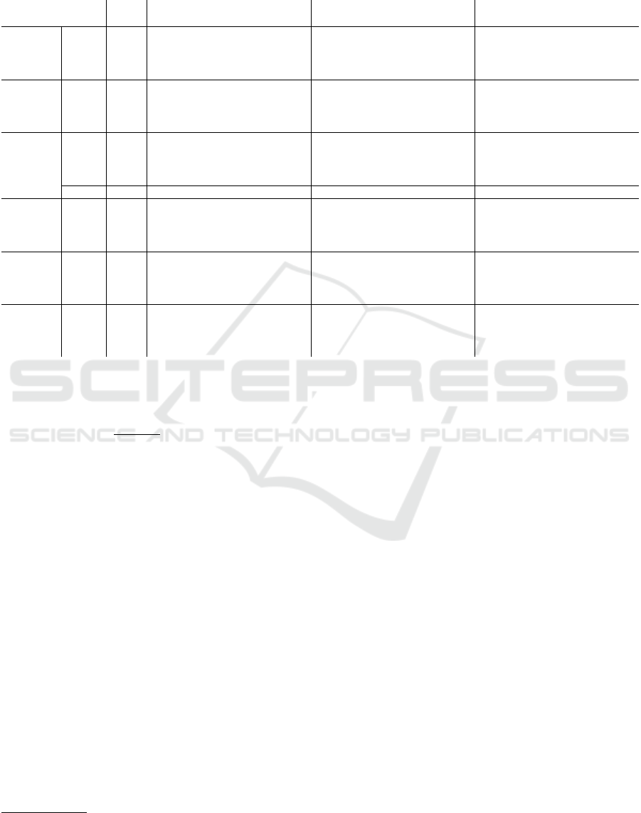
Table 1: Ratio of used vertices, ratio of solved instances, sum of IPC score, ratio of instances solved optimally, average number

of conﬂicts, and average number of constraints. The results are split by the map type. Strategies are baseline (B), prune-and-

cut (P), makespan-add (M), and combined (C). Approaches to choosing shortest paths are single-path (SP), all-paths (AP),

random-paths (RP), and distant-paths (DP).

P C M

type SP AP RP DP SP AP RP DP SP AP RP DP

Used

vertices

empty 1 0.14 0.23 0.21 0.23 0.15 0.24 0.22 0.23 0.19 0.24 0.23 0.24

maze 1 0.18 0.2 0.18 0.19 0.20 0.22 0.21 0.21 0.22 0.22 0.22 0.22

random 1 0.19 0.27 0.24 0.25 0.22 0.3 0.28 0.29 0.25 0.31 0.3 0.31

room 1 0.21 0.24 0.22 0.22 0.23 0.27 0.25 0.25 0.24 0.29 0.27 0.28

Solved

instances

empty 0.78 0.99 0.81 0.84 0.82 1.00 0.81 0.84 0.82 0.87 0.81 0.82 0.8

maze 0.85 0.87 0.88 0.87 0.87 0.98 0.97 0.97 0.98 0.94 0.94 0.94 0.94

random 0.79 0.91 0.82 0.84 0.84 1.00 0.89 0.92 0.91 0.93 0.87 0.89 0.88

room 0.8 0.83 0.81 0.82 0.82 0.97 0.92 0.95 0.94 0.89 0.89 0.89 0.89

∑

IPC

empty 874.6 1930.5 1312.8 1081.7 1086.3 2395.2 1276.5 1406.7 1324.4 1517.9 1275.8 1312.5 1279.2

maze 890.1 1153.2 1123.6 1128.3 1143.3 1775.5 1633.8 1752.8 1754 1475.7 1452.6 1470.5 1466.1

random 886 1668.0 1110.2 1049.9 1102.3 2275.5 1422.4 1594.6 1551.5 1560.7 1300.3 1374.2 1324.4

room 877.3 1386.4 1007.5 1191.6 1179.5 2078.3 1594.5 1850.6 1828.7 1474 1382.6 1461.9 1442

total 3527.9 6138.1 4554.1 4451.6 4511.4 8524.5 5927.2 6604.6 6458.6 6028.4 5411.3 5619.2 5511.6

Solved

optimally

empty - - - - - 0.93 1.00 1.00 1.00 1.00 1.00 1.00 1.00

maze - - - - - 0.91 0.94 0.92 0.92 0.92 0.93 0.93 0.93

random - - - - - 0.89 0.97 0.95 0.96 0.86 0.91 0.91 0.91

room - - - - - 0.86 0.93 0.91 0.92 0.76 0.86 0.85 0.85

Conﬂicts

empty 133 97 148 131 136 111 147 141 142 139 148 146 148

maze 2457 1239 1804 1274 1265 3101 2969 3120 3143 3361 3482 3443 3354

random 206 193 195 174 173 218 235 234 227 448 458 460 459

room 1007 402 313 270 289 1642 1414 1513 1423 1525 1400 1527 1545

Constraints

[millions]

empty 4.7 7.3 5.1 5.9 5.2 7.4 5.1 6 5.2 6 5.0 5.2 5.0

maze 6.0 6.1 6.4 6 6.2 6.4 6.8 6.5 6.6 6.8 6.8 6.8 6.8

random 5.4 5.9 6 6 6 6 6.1 6.1 6.1 6.1 5.8 6 5.8

room 4.8 5.4 5.6 5.4 5.4 5.7 5.9 5.8 5.7 5.7 5.9 5.9 5.9

B performs worse than any other used combination.

Similar results can be seen when exploring the IPC

score

(Computed as 0 if the solver did not ﬁnish in

time, otherwise as

min. time

solver time

, where min. time is the

time it took the fastest solver and solver time is the

time it took the solver in question. The score ranges

from 0 to 1, where the bigger the number the bet-

ter. The scores of all instances are summed.) For the

P strategy the AP approach performs better than DP

and RP, meaning that while it did not solve more in-

stances, the instances it managed to solve were solved

faster. For the other strategies, the order remains the

same as with the number of solved instances. It is

unsurprising that the suboptimal strategies achieved a

better score that the optimal P.

We argue that these results stem from the number

of used vertices. By exploring the ASP solver, we

see that for all strategies and all additional shortest

path approaches, the number of conﬂicts stays mostly

within the same order of magnitude as for SP. Hence,

ASP search difﬁculty remains unchanged. However,

compared to SP, the other approaches add more ver-

tices to the restricted graph to consider and, in con-

sequence, this increases the grounding time of clingo

which, in turn, leads to more timeouts.

The new shortest path approaches reduce the size

introduced at International Planning Competition.

of the internal problem speciﬁcation in terms of the

number of constraints. We conjecture that since the

new approaches generally select multiple (and more

likely exclusively usable by one agent) vertices for

the restricted graph, the amount of constraints encod-

ing possible agent collisions is reduced. However, as

mentioned above, this has no signiﬁcant impact on the

search complexity.

We also explore the quality of the solutions pro-

duced by the suboptimal strategies. The ratio of in-

stances solved optimally is again shown in Table 1.

Strategy C is more often optimal compared to M.

This time, we can see the beneﬁt of adding extra ver-

tices to the restricted graph. The most often optimal

approach is AP closely followed by RP and DP, while

SP achieved the worst results. The difference is again

less prominent on maze maps.

7 CONCLUSION

We extended the study on pruning maps to increase

the efﬁciency of reduction-based MAPF solvers. In

the original paper, only one random path was cho-

sen for each agent to build a restricted graph. Con-

versely, in this paper, we proposed several approaches

to choosing multiple different paths for each agent,

Multi-Agent Pathﬁnding on Large Maps Using Graph Pruning: This Way or That Way?

205

providing the underlying solver with more choices. In

theory, this should make it possible for the agents to

avoid collisions more easily. In our experiments, we

found that this rarely happens and that it is more ben-

eﬁcial to provide the solver with just one random path

making the relaxed instances simpler for the cost of

possibly having to solve more relaxations. Thus, we

showed that the original approach is justiﬁed, a result

that is lacking in the original study. On the other hand,

we also showed that providing the agents with more

possible paths leads more often to an optimal solution

when using one of the suboptimal strategies.

ACKNOWLEDGEMENTS

Research is supported by project P103-19-02183S of

the Czech Science Foundation, the Czech-USA Co-

operative Scientiﬁc Research Project LTAUSA19072,

and DFG grant SCHA 550/15, Germany.

REFERENCES

Gebser, M., Kaminski, R., Kaufmann, B., Lindauer, M., Os-

trowski, M., Romero, J., Schaub, T., and Thiele, S.

(2019). Potassco User Guide, 2.2.0.

Gebser, M., Obermeier, P., Otto, T., Schaub, T., Sabuncu,

O., Nguyen, V., and Son, T. (2018a). Experiment-

ing with robotic intra-logistics domains. Theory and

Practice of Logic Programming, 18(3-4):502–519.

Gebser, M., Obermeier, P., Schaub, T., Ratsch-Heitmann,

M., and Runge, M. (2018b). Routing driverless trans-

port vehicles in car assembly with answer set pro-

gramming. Theory and Practice of Logic Program-

ming, 18(3-4):520–534.

omez, R. N., Hern

andez, C., and Baier, J. A. (2021). A

compact answer set programming encoding of multi-

agent pathﬁnding. IEEE Access, 9:26886–26901.

acker, C., Bouros, P., Chondrogiannis, T., and Althaus,

E. (2021). Most diverse near-shortest paths. In 29th

International Conference on Advances in Geographic

Information Systems, pages 229–239. ACM.

Hanaka, T., Kobayashi, Y., Kurita, K., Lee, S. W., and

Otachi, Y. (2021). Computing diverse shortest paths

efﬁciently: A theoretical and experimental study.

CoRR, abs/2112.05403.

Hus

ar, M., Svancara, J., Obermeier, P., Bart

ak, R., and

Schaub, T. (2022). Reduction-based solving of

multi-agent pathﬁnding on large maps using graph

pruning. In 21st International Conference on Au-

tonomous Agents and Multiagent Systems, pages 624–

632. IFAAMAS.

Kaminski, R., Romero, J., Schaub, T., and Wanko, P.

(2022). How to build your own ASP-based sys-

tem?! Theory and Practice of Logic Programming,

23(1):299-361.

Kornhauser, D., Miller, G. L., and Spirakis, P. G. (1984).

Coordinating pebble motion on graphs, the diame-

ter of permutation groups, and applications. In 25th

Annual Symposium on Foundations of Computer Sci-

ence, pages 241–250.

Li, J., Tinka, A., Kiesel, S., Durham, J. W., Kumar, T.

K. S., and Koenig, S. (2020). Lifelong multi-agent

path ﬁnding in large-scale warehouses. In 19th Inter-

national Conference on Autonomous Agents and Mul-

tiagent Systems, pages 1898–1900. IFAAMAS.

Nguyen, V., Obermeier, P., Son, T. C., Schaub, T., and Yeoh,

W. (2017). Generalized target assignment and path

ﬁnding using answer set programming. In 26th In-

ternational Joint Conference on Artiﬁcial Intelligence,

pages 1216–1223. ijcai.org.

Ratner, D. and Warmuth, M. K. (1990). NxN puzzle

and related relocation problem. J. Symb. Comput.,

10(2):111–138.

Sharon, G., Stern, R., Goldenberg, M., and Felner, A.

(2011). The increasing cost tree search for optimal

multi-agent pathﬁnding. In 22nd International Joint

Conference on Artiﬁcial Intelligence, pages 662–667.

Silver, D. (2005). Cooperative pathﬁnding. In Artiﬁ-

cial Intelligence and Interactive Digital Entertain-

ment, pages 117–122.

Stern, R., Sturtevant, N. R., Felner, A., Koenig, S., Ma, H.,

Walker, T. T., Li, J., Atzmon, D., Cohen, L., Kumar,

T. K. S., Bart

ak, R., and Boyarski, E. (2019). Multi-

agent pathﬁnding: Deﬁnitions, variants, and bench-

marks. In 12th International Symposium on Combi-

natorial Search, pages 151–159. AAAI Press.

Surynek, P. (2019). Unifying search-based and

compilation-based approaches to multi-agent

path ﬁnding through satisﬁability modulo theories.

In 28th International Joint Conference on Artiﬁcial

Intelligence, pages 1177–1183. ijcai.org.

Svancara, J. and Bart

ak, R. (2019). Combining strengths of

optimal multi-agent path ﬁnding algorithms. In 11th

International Conference on Agents and Artiﬁcial In-

telligence, pages 226–231. SciTePress.

Yu, J. and LaValle, S. M. (2013). Structure and intractability

of optimal multi-robot path planning on graphs. In

27th AAAI Conference on Artiﬁcial Intelligence.

ICAART 2023 - 15th International Conference on Agents and Artiﬁcial Intelligence

206