TSCH Slotframe Optimization Using Differential Evolution Algorithm

for Heterogeneous Sensor Networks

Aida Vatankhah, Ramiro Liscano and Tarana Ara

Dept. of Electrical, Computer, and Software Engineering, Ontario Tech University, Oshawa, Canada

Keywords:

Time-Slotted Channel Hoping, IEEE 802.15.4e, Slotframe Length, DE Optimization, Throughput, Network

Delay.

Abstract:

The Time-Slotted Channel Hopping (TSCH) from the IEEE 802.15.4 standard aims at providing high reli-

ability to industrial wireless networks. One of the most signiﬁcant challenges in TSCH is determining the

schedule. In this paper, we present an algorithm to ﬁnd an optimal TSCH schedule with the minimum slot-

frame size that can meet the desired throughput of each node. A customized Differential Evolution (DE)

optimization algorithm was developed based on the determination of an interference and collision free trans-

mission graph which has not been used in prior works. Our schedule can encompass sensors with different

packet rates and results in a low transmission delay of the data packets. Using Matlab, we performed various

complexity analysis to measure the time it takes to ﬁnd the optimal schedule in different scenarios. Addition-

ally, we implemented the optimal TSCH schedule on TSCH-SIM simulator to conﬁrm that the schedule is

working promising. As a result, the high value of the Packet Delivery Rate (PDR) obtained from the simula-

tions veriﬁed the schedule performance.

1 INTRODUCTION

TSCH is a synchronous MAC (Medium Access Con-

trol) protocol, speciﬁed in the IEEE 802.15.4 standard

amendment (Watteyne et al., 2016). To provide more

reliability to upper network layers, TSCH (IEEE Std

802.15.4-2011, 2011) (Howitt and Gutierrez, 2003)

combines Time Division Multiple Access (TDMA)

and Frequency Division Multiple Access mechanisms

(FDMA). Former allows several users to share the

same frequency channel by dividing the signal into

different time slots, while latter allows multiple users

to send data through a single channel by dividing the

channels’ bandwidth into separate non-overlapping

sub-channels and allocating each sub-channel to a

separate user. In other words, TDMA separates users

by time and FDMA separates users by frequency.

In TSCH, medium access is orchestrated by a

schedule that is distributed to all the nodes in the

network. The network coordinator is responsible for

management and control of trafﬁc ﬂows and also it

computes the optimized time slot and channel assign-

ment (Urke et al., 2021). (Teles Hermeto et al., 2017).

For each pair of nodes, a cell in the schedule is allo-

cated to specify when and in which channel the trans-

missions will take place. A cell is indicated by a tu-

ple as (timeslotOffset, channelOffset) and it can be

shared by multiple transmissions or dedicated to only

one transmission. The standard does not deﬁne how

TSCH packet transmission schedule is deﬁned (Urke

et al., 2021).

Industrial sensor networks are expected to accom-

modate sensors with different packet rates, and this

makes it particularly challenging to determine an op-

timal transmission schedule for the network. For in-

stance, consider two sensors generating 4 and 100

packets/sec, respectively. Determining an optimal

slotframe length for the ﬂows is important, since a

short slotframe length results in too many repetitions

of a slotframe prior to the data generation, whereas a

schedule with a long slotframe will suffer high end-

to-end delays. Consequently, the slotframe should

be long enough to include all the required transmis-

sions by considering the estimated number of gener-

ated packets.

In this paper, we propose a novel slotframe length

optimization for TSCH scheduling based on the Dif-

ferential Evolution (DE) algorithm to minimize the

overall network delay while maintaining the expected

packet transmissions in the network. Delay optimiza-

tion problem is identiﬁed as a combinatorial optimiza-

tion problem and is known to be NP-hard (Ojo and

Vatankhah, A., Liscano, R. and Ara, T.

TSCH Slotframe Optimization Using Differential Evolution Algorithm for Heterogeneous Sensor Networks.

DOI: 10.5220/0011623400003399

In Proceedings of the 12th Inter national Conference on Sensor Networks (SENSORNETS 2023), pages 57-66

ISBN: 978-989-758-635-4; ISSN: 2184-4380

 2023 by SCITEPRESS – Science and Technology Publications, Lda. Under CC license (CC BY-NC-ND 4.0)

Giordano, 2016) (Abu-Khzam et al., 2015). In this

paper we leveraged the DE optimization algorithm to

determine a sub-optimal schedule in terms of delay

for a centralized managed heterogeneous sensor net-

work. DE is a random search algorithm based on pop-

ulation evolution, proposed by Storn and Price (Storn

and Price, 1997). This method performs optimiza-

tion by iteratively trying to improve a candidate solu-

tion regarding a given measure of quality. It has been

proven that DE is a reliable optimization strategy for

many different tasks. In our problem the DE opti-

mizer has to generate a number of schedules that are

evaluated using an objective function to determine the

best schedule.

This paper is structured as follows. Section 2 is a

review of related works. Section 3 focuses on the pro-

posed slotframe optimization using the customized

DE optimization algorithm for TSCH and highlights

the details of each step. The optimized schedule for

a speciﬁc network topology is described in section 4

and the simulation results extracted from TSCH-SIM

simulator are presented in section 5. Then, a time

complexity analysis of the algorithm is performed in

section 6. Finally, section 7 concludes this paper.

2 RELATED WORK

A conﬂict-free scheduling algorithm was proposed in

(Soua et al., 2016), which targets the minimization of

transmission delay by reducing the slotframe length.

The author introduced the concept of ”WAVES”;

which is a period where each node performs at least

one packet transmission during the WAVE time. As a

result, the slotframe length will be equal to the time

when all the packets of each node are sent. In this

paper, the nodes closer to the sink suffer high traf-

ﬁc overﬂows or queue overﬂow, and some nodes will

suffer high delays in large networks. The packet rate

of nodes is assumed to be homogeneous, although the

total number of packets received from child nodes is

different from others.

A debt-based scheduler is presented in (Minet

et al., 2018). In this approach, a debt value is cal-

culated for each TSCH device which has a message

to transmit, that is equal to the multiplication of the

remaining number of data messages the node has to

transmit and the depth of device in the network. No

spatial reuse was applied on cells in this paper, that

is, a cell is granted to only one transmitter which re-

sults in including lower number of transmissions in a

single time slot and higher delays accordingly. Simi-

larly, Ines Khouﬁ et al. (Khouﬁ et al., 2017) proposed

a multi slotframe to determine the lower bound num-

ber of slots required to perform data gathering and to

support sensor ﬂows with data delivery constraints.

These two approaches (Khouﬁ et al., 2017) (Minet

et al., 2018) only allocate one cell per node to han-

dle all trafﬁc. Therefore, the performance of the algo-

rithm degrades under high trafﬁc loads.

A centralized Adaptive Multi-hop Scheduling

(AMUS) algorithm has been proposed in (Jin et al.,

2016) to provide optimized schedules using tentative

cell allocations. AMUS reserves additional cells for

those links which might be heavily loaded, or prone

to interference to improve communication reliability

and achieve low latency. A Combinatorial Multi-

Armed Bandit (CMAB) was proposed in (Javan et al.,

2019) which determines the optimal scheduling by

assignment of TSCH cells to links using the Linear

Learning Rewards (LLR) algorithm. This is done

using a bipartite graph that matches non-interfering

links to slot-frame matrix cells. We also use a graph

to represent non-interfering links but optimize this us-

ing a DE algorithm.

The Trafﬁc Aware Scheduling Algorithm (TASA)

(Palattella et al., 2012) aims at ﬁnding the minimal

number of slots needed to send all data to a root node.

To reach this goal, matching and coloring functions

are used to plan the distribution of slots and channels

across the entire network without any collision. First,

links that still have data to transmit are selected at the

corresponding time slot through a matching process.

Then, the channel offsets of the links are allocated so

that interference does not occur through the matching

process.

The effect of different slotframe length on energy

consumption is investigated in (Kharb and Singhrova,

2018), however, the goal of this paper is to ﬁnd the

minimum slotframe length that results in minimum

energy consumption. Hill Climbing technique as a lo-

cal search based mathematical optimization was used

to discover the optimized slotframe length and the

penalty function is used to provide a hill to climb

when the optimization starts at undesirable location.

The simulation results show that slotframe length and

energy consumption have inverse correlation relation-

ship.

Fafoutis et al. (Fafoutis et al., 2018) proposed

an adaptive static scheduling that allows each pair of

nodes to control their active time slots in a distributed

manner in order to improve the energy efﬁciency of a

TSCH network. A static scheduler was built at com-

pilation time with excessive time slots over alloca-

tion yet, the nodes can dynamically activate or deac-

tivate their a priori allocated time slots, according to

the trafﬁc requirements. However, the authors did not

consider the cost of blind over-provisioning in terms

SENSORNETS 2023 - 12th International Conference on Sensor Networks

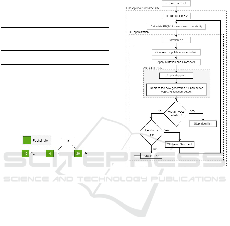
Table 1: List of notations used in this paper.

Symbol Description

Sensor with ID i

Set of vectors includes all the collision and interference

free transmissions as a pair of transmit-receive tuple

m Size of space vector V

Matrix that keeps track of the interference and collision

between transmissions

i, j

Transmission status of i and j’th pairs in V

s f

Slotframe length

Number of timeslots in the slotframe

PR(S

) Packet rate of sensor S

EP(S

) Expected generated packets for sensor node S

of delay performance.

3 METHODOLOGY

To explain the algorithm, we use a simple tree topol-

ogy as shown in Figure 1, consisting of a root

node labeled as S

and three other sensor nodes as

, S

}. In this ﬁgure the green boxes show the

number of packets each node generates in one second.

Figure 1: A simple tree topology consisting of 3 sensor and

a root node.

In our context, the TSCH schedule is built with

the concept of spatial reuse that allows each cell to be

shared by multiple transmissions. Multiple transmis-

sions allocation to a single cell will diminish delay

due to the capability of encompassing higher number

of transmissions in each time slot; however, it can also

lead more potential collisions and interference while

exchanging data. To address this concern, we have

deﬁned a FreeSet graph that captures transmissions

among pairs of nodes that are collision and interfer-

ence free. The transmissions in one set of the FreeSet

can be assigned to a cell in TSCH schedule without

causing any collision or interference.

Then, the expected number of transmissions is es-

timated for each sensor node according to its packet

rate as well as its children’s packet rate since each

node is also responsible to relay the received packets

from its children. Using a customized DE optimiza-

tion algorithm, we found the minimum slotframe size

that includes all the required estimated transmissions.

Figure 2 is a ﬂowchart describing the overall opti-

mization procedure. In the following sections, each

step of the algorithm is explained in more detail. The

list of symbols and notations used in this paper is pre-

sented in table 1.

Figure 2: Flowchart for customized DE slotframe size opti-

mization.

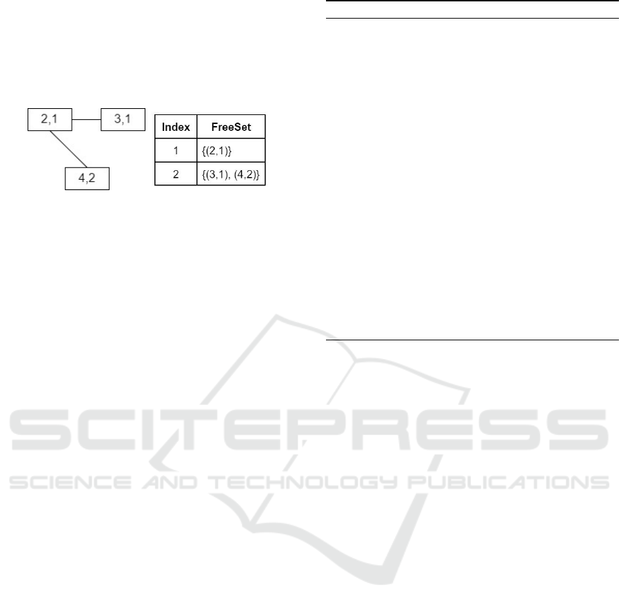
3.1 Creating the FreeSet Graph

Before applying the customized DE optimization,

FreeSet is created, which consists of several set of

node pairs that can be assigned to a single cell without

causing any collision or interference. Assuming that

A includes a set of transmissions as {A

, ..., A

}, A

consists of the transmission / receive pair as S

→ S

where j and k correspond to the node index values. In

this case:

• A new transmission can be assigned to the same

cell which is appointed to A only if it does not

have any collision or interference with any of the

transmissions in set A.

• The new transmission can be assigned to the same

time slot which A has been assigned to, providing

that it does not cause any collision with any of

transmissions in A.

The union of collision and interference graph for

the sample topology is depicted in Figure 3a. In this

graph, the transmissions connected through an edge

cannot be assigned to an identical cell as it will cause

TSCH Slotframe Optimization Using Differential Evolution Algorithm for Heterogeneous Sensor Networks

collision or interference. For instance, transmissions

→ S

and S

→ S

are not allowed to be assigned

to a single cell or time slot, since node S

cannot send

and receive at the same time. As shown in Figure 3b,

FreeSet is obtained from the complement of the graph

3a.

(a) . (b) .

Figure 3: Union of the collision and interference graph (a)

FreeSet (b).

As shown in Algorithm 1, we implemented the

FreeSet graph as a vector space V that includes all

the collision and interference free transmissions as a

pair of transmit-receive tuple. Based on the example

in Figure 1, this set would include the 3 transmissions

as V = { S

→ S

, S

→ S

, S

→ S

We use a matrix as M to keep track of the interfer-

ence and collision between transmissions, where M

i, j

represent the status of transmission pairs i and j in V .

The values in the matrix can be 0, 1, or 2. A value

of 0 implies that transmission i and j can be assigned

to the same cell; a value of 1 implies that there will

be interference if these two pairs transmit packets si-

multaneously but they can transmit their packets in

different channels to avoid interference; a value of 2

implies that if the pair i and j transmit a packet at the

same time collision will occur. Based on these values,

collision and interference can be distinguished.

Below is an algorithm that creates the FreeSet

from the vector V . The complexity of this algorithm

is O(m · log(m − 1)) where m denotes the size of set

V .

3.2 Estimate the Expected Number of

Packets Generated

A TSCH slotframe consists of several time slots and

slotframe length can be calculated by multiplying the

number of time slots in a slotframe by the time slot

length. The slotframe should be large enough to trans-

mit all the estimated number of packets within the

slotframe time period. Nodes are synchronized and

follow a schedule using a slotframe that continuously

repeats over time.

For any particular slotframe, we estimate the num-

ber of packets that are to be transmitted in the network

by computing the number of packets generated in that

speciﬁc slotframe size and propagating this through-

Algorithm 1: Creating FreeSet.

Input V = {V

, ...,V

}

Output FreeSet

1: M

c∗c

∈ ℜ

: c = 1...m, m = |V |

2: for i = 1 : m do

3: Pair

← V

4: for j = i + 1 : m do

5: Pair

← V

6: Check the conditions for Collision and Inter-

ference for Pair

and Pair

7: if (Pair

, Pair

) in collision then

8: M

i, j

← 2

9: else if (Pair

, Pair

) in interference then

10: M

i, j

← 1

11: else

12: M

i, j

← 0

13: end if

14: end for

15: end for

16: FreeSet ← Pairs in M with value 1

17: return FreeSet

out the network topology. As example the simple

3 node topology shown in Figure /refﬁg:4-nodes is

considered. The generated packet rate of these three

nodes {S

, S

} is {4, 20, 10} packets/sec, respec-

tively. For the scheduler, we assume that all the data

packets have been generated simultaneously after the

network initialization phase. The highest delay that

can exist is the case where a node generates a data

packet and has to wait for the next slotframe to trans-

mit. To avoid high delays, we estimate the number of

cells each node needs according to its packet rate and

their children’s packet rate.

Considering a slotframe length as L

s f

consisting

of N

time slots, one can estimate the generated pack-

ets during the slotframe for each node S

as EP(S

) us-

ing Equation 1. The result obtained from L

s f

· PR(S

)

may be a fraction, although we need an integer value

as the output for the expected number of generated

packets. The most conservative approach to deal with

fractions is to round up, which results in over schedul-

ing of transmissions. Any other approach can orig-

inate the possibility missing a required transmission

which cause an eventual queue overﬂow. After the

number of packets generated during a particular slot-

frame size is calculated, the number of packets gener-

ated by the children are summed up as can be seen in

Equation 1.

EP(S

) = ⌈L

s f

· PR(S

)⌉ +

∑

j=1

EP(S

.child( j )) (1)

where PR(S

) denotes the packet rate of sensor node

SENSORNETS 2023 - 12th International Conference on Sensor Networks

and S

.child( j ) represents the j

child of node S

Slotframe length L

s f

is calculated through the follow-

ing equation:

s f

= L

· N

(2)

where L

is time slot length that is assumed as stan-

dard value of 10 ms and N

denotes the number of

time slots in a slotframe.

3.3 Customization of the DE

Optimization Algorithm

Using different channel offsets in TSCH schedule

provides the opportunity for the interfering transmis-

sions to be concurrently done without interference.

Consequently, although we cannot schedule transmis-

sions that collide with each other in the same time

slot, we can schedule interfering transmissions in

same time slot but on different channel offsets.

In initialization step of the DE optimization algo-

rithm, the minimum population size is used to reduce

the complexity of the computations. Minimally, 4

random solutions are generated in the search space

of the DE optimization problem. Search space in

our problem is set of transmissions in FreeSet; each

can be of a different size which is not possible con-

dition in Differential Evolution optimization process

and was explained in details in (Vatankhah and Lis-

cano, 2022).

In the Mapping phase, each value in the gener-

ated matrix is mapped to a transmission set in the

FreeSet which is described thoroughly in (Vatankhah

and Liscano, 2022). A node is labeled as SATISFIED

or NOT SATISFIED which declares whether the sufﬁ-

cient number of cells have been assigned to the sensor

node S

based on the calculated EP(S

) value or not.

Moreover, while generating a schedule in the

Mapping phase, we utilized a prioritization for choos-

ing between two transmissions that collide in same

time slot but different channels. While checking each

time slot for possible collisions, we may discover

transmissions causing a collision such as (S

, S

) and

, S

) due to the identical destination node. Trans-

mission (S

, S

) will be chosen over the other trans-

mission only if one of the circumstances listed below

is met:

• S

is labeled as SATISFIED

• EP(S

) >= EP(S

)

Providing that either conditions are met, (S

, S

)

will be removed from the schedule. Afterwards, the

schedule passes through the Mutation and Crossover

phases of the DE algorithm. The details of Muta-

tion and Crossover have been thoroughly explained

in (Vatankhah and Liscano, 2022).

In the Selection phase, the generated schedule is

compared to the existing one that was generated in

initialization phase as shown in Equation 3. In this

stage, the schedule with the higher objective function

value will survive and will be replaced with the corre-

sponding schedule. The objective is to maximize the

Equation 3.

f (x) = Num(

∑

i=1

.lbl == SAT ISFIED) (3)

where S

.lbl is equal to SATISFIED only if the

number of cells that are assigned to sensor S

is more

or equal to the EP(S

). This function calculates the

number of nodes that are labeled as SATISFIED. The

algorithm will continue running on a speciﬁc slot-

frame length until all the sensor nodes labeled as SAT-

ISFIED or the iteration exceeds an iteration maximum

value which has been set to 20 in the examples pre-

sented in this paper. If this maximum value is reached

the optimization process will resume using a new slot-

frame size which is larger than the original one by one

slot.

As depicted in Figure 2, block titled ”DE opti-

mization” shows when all the nodes are SATISFIED,

the optimization is terminated, otherwise, slotframe

size will increase by one and DE optimization will try

to ﬁnd a schedule that can satisfy all the nodes.

4 AN OPTIMIZED SCHEDULE

SCENARIO

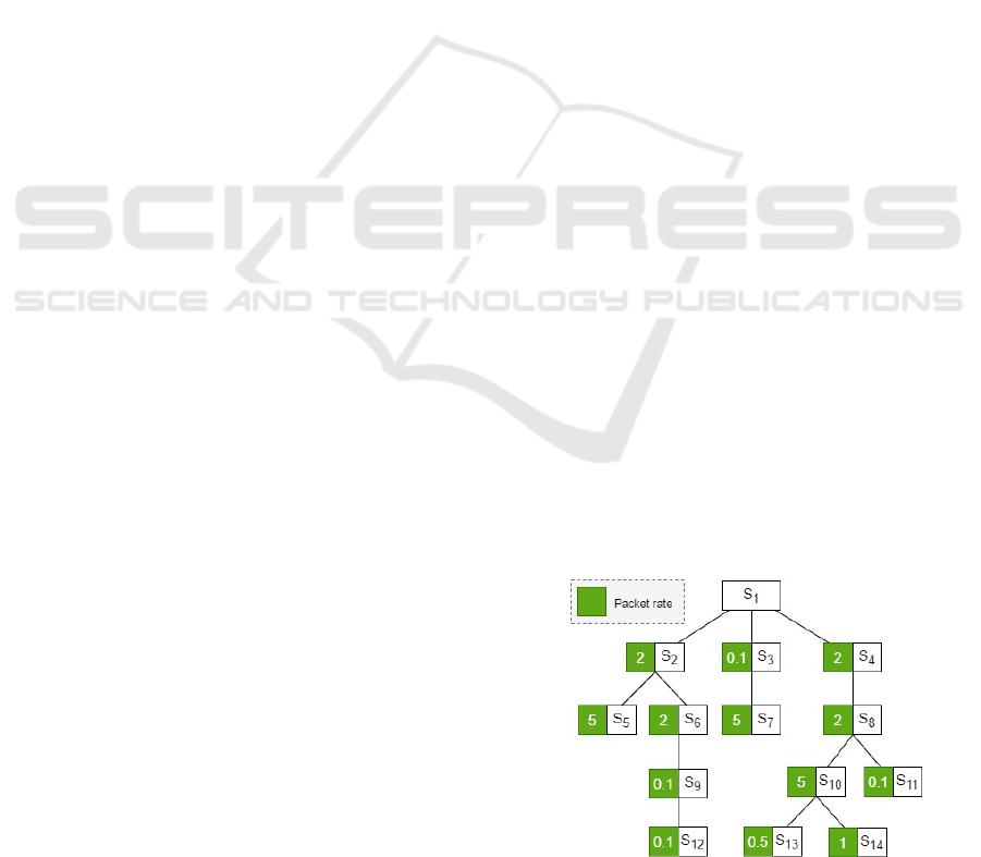
To evaluate the performance of the algorithm on het-

erogeneous trafﬁc ﬂows, a tree topology consisting of

14 nodes with the given packet rates was examined as

shown in Figure 4, where the green boxes denote the

packet rate of each node.

Figure 4: A sample tree topology of 14 sensor nodes.

TSCH Slotframe Optimization Using Differential Evolution Algorithm for Heterogeneous Sensor Networks

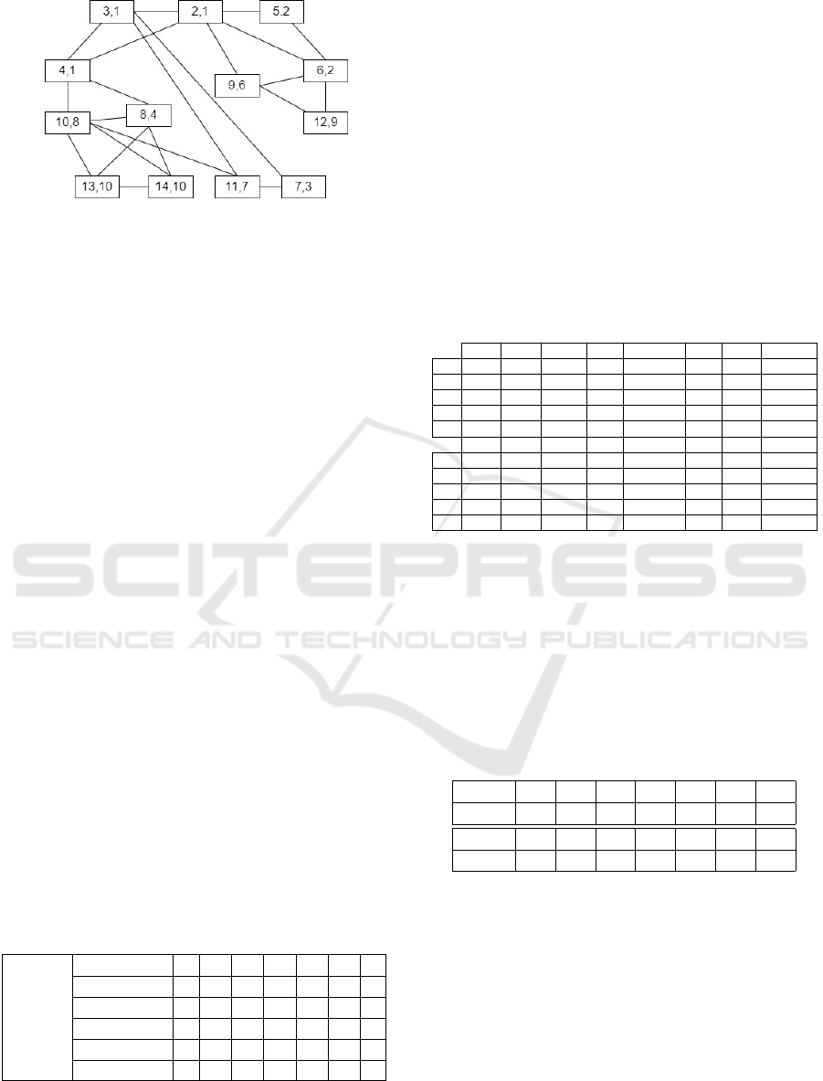
Figure 5: Union of collision and interference graph for the

network depicted in Figure 4.

According to the given topology, the possible

transmissions are {(S

, S

), (S

, S

), (S

, S

), (S

, S

), (S

, S

), (S

, S

), (S

, S

), (S

, S

), (S

, S

), (S

, S

), (S

, S

)} which are shown as

graph vertices in Figure 5. Based on the collision and

interference rules explained in section 3.1, the colli-

sion and interference graph was established as Figure

For each slotframe size, the proposed algorithm

calculates the number of expected packets for each

node. Then, the Customized DE algorithm explores

to ﬁnd a solution that can accommodate all the ex-

pected number of transmissions. The expected num-

ber of generated packets for each node is calculated

using Equation 1.

In this example, any fractional values are rounded

up to the nearest integer. In this table, the number

of generated packets and the number of the assigned

cells for sensor nodes {S

, S

, ..., S

} are shown in

the EP and ASSIGNED rows, respectively. From Ta-

ble 2, it can be observed that the number of assigned

cells in the optimized schedule is more or equal to the

expected packet transmission values for each sensor

node. The higher number of assigned transmissions

for some nodes in the schedule is due to the fact that

some of the NOT SATISFIED transmissions are co-

located with SATISFIED transmissions in the same

set of FreeSet. When the schedule tries to add the

NOT SATISFIED transmission to the schedule, it also

adds the already SATISFIED transmission.

Table 2: Expected number of packet generation for slot-

frame of size 15.

s f

= 15

ID S

5 2 6 1 3 1 5

ASSIGNED 6 3 6 4 5 12 6

ID S

2 3 1 1 1 1

ASSIGNED 3 3 4 10 8 1

For the given example in Figure 4, the algorithm

terminates at a slotframe size of 15, when all the

nodes are labeled as SATISFIED and Table 2 shows

the expected and assigned transmissions for each of

the slots. One can observe that the number of assigned

slots is higher or equal to the expected.

After these assignments the TSCH schedule in-

cludes all the required number of transmissions to

transmit the generated packets or relay the received

packets from their children as illustrated in Table 3.

In this table, multiple transmissions are scheduled to

send their packets in the speciﬁed time slot and chan-

nel offset. For instance, sensor nodes S

, S

and S

are scheduled to transmit or relay the packets to nodes

, S

and S

, respectively, in time slot 2 and channel

offset 3.

Table 3: Schedule for the optimal slotframe size of 15.

ts 1 ts 2 ts 3 ts 4 ts 5 ts 6 ts 7 ts 8

ch 1 11 6 11,13

ch 2 13 2,7,12

ch 3 8 3 9

ch 4 2 8 12 2,7,12

ch 5 2,7,12 8 7, 9, 13 12,13 2,7 6,3,8 8 10,2,7,12

ts 9 ts 10 ts 11 ts 12 ts 13 ts 14 ts 15

ch 1 4

ch 2 4,7,13 4,5

ch 3 6,3,8 4,5 4,5 11,7,12,13 11,13 4,13

ch 4 14 5,9 10 6

ch 5 12 10,7,12 7,12 6 7,12 7,12

As explained earlier, the customized DE optimiza-

tion initialized by setting slotframe length L

s f

to 3.

For the given topology, the number of SATISFIED

nodes is 6 out of 14 nodes as presented in Table 4.

The slotframe length increases by one in this case un-

til all the nodes are SATISFIED. As it can be observed

from Table 4, the schedule with slotframe length of 15

is found while all the 14 nodes are satisﬁed.

Table 4: Maximum number of SATISFIED nodes for each

slotframe length.

s f

3 4 5 6 7 8 9

#SAT 6 9 9 10 10 11 12

s f

10 11 12 13 14 15

#SAT 13 13 13 13 13 14

5 SIMULATION

To evaluate the performance of the schedule obtained

from our Customized DE optimization algorithm,

we implement the optimized schedule in the TSCH-

Sim (Elsts, 2020) network simulator for the scenario

shown in Figure 4. The overall throughput and aver-

age delay of the network are measured using TSCH-

SIM simulator.

By network throughput, we deﬁne this as the total

SENSORNETS 2023 - 12th International Conference on Sensor Networks

Table 5: Simulation parameters used for the TSCH DE op-

timized schedule.

Parameter Value

SIMULATION DURATION 2500 sec

APP WARMUP PERIOD SECOND 1000 sec

LINK MODEL Logistic Loss model

TRANSMIT RANGE M 40 meters

APP PACKET SIZE 100

MAC MAX RETRIES 7

MAC QUEUE SIZE 15

ROUTING ALGORITHM ManualRouting

SCHEDULING ALGORITHM ManualScheduler

SLOT FRAME LENGTH 15

TIME SLOT DURATION 10 ms

number of packets successfully received at the root

node in a given time and one would expect this to be

the sum of all the data packet generation rates. The

mathematical expression for throughout is speciﬁed

as below.

Overall throughput =

∑

i=1

received packets

total simulation time

(4)

where N denotes the total number of packets and

received packets

is the number of packets received

by sensor S

Network delay refers to the total time (propaga-

tion, transmission, queuing, and processing period) a

packet takes to travel from a source node to a des-

tination node and it is estimated in seconds. In this

simulator, the delay is evaluated by taking the differ-

ence between the time a packet is generated and is

successfully received by the root node. The average

delay has been calculated utilizing Equation 5.

Delay =

∑

i=1

(time(i)

received

−time(i)

generated

)

total packets

(5)

We manually conﬁgured the network with the

nodes’ positions, connections and routes shown in

Figure 4. These values match those used to deter-

mine the optimal schedule. We chose the Logistic

Loss model as the radio propagation model. For the

experiment, we considered ﬁve channel offsets and 15

time slots with each time slot duration of 10 millisec-

onds again matching the settings and results obtained

from the customized DE optimization in Matlab. The

details of the simulation parameters are listed in Table

In table 5, APP WARMUP PERIOD SECOND is

the time period it takes for all the sensor nodes to join

the network (i.e when the network is stable). Data

packets are not generated before this warm-up period

has ended after the start of the simulation resulting

in more accurate metrics. The MAC re-transmissions

Table 6: Analysis of the proposed customized DE optimiza-

tion algorithm.

Evaluation Parameters Customized DE Algorithm

PDR 99.75%

Total Generated Packets 22349

Received Packets 22295

Average Delay (sec) 3.2

Maximum Delay 4

Minimum Delay 2.4

Throughput 14.1

were left as the default value of 7, however, the MAC

queue size was increased to 15 to eliminate pack-

ets being dropped from queue overﬂows. Simulation

time was set to 2500 seconds which 1000 seconds of

this time is the warm up period. Application packet

size was considered as 100 bytes and the standard

value for time slot was used as 10 ms. The optimal

slotframe size for the schedule was obtained as 15

time slots which implies 150 ms.

5.1 Simulation Results

We used the overall throughput, average end-to-end

delay, Packet Delivery Ratio (PDR) as metrics to con-

ﬁrm the efﬁciency of the proposed approach. Accord-

ing to the results given in Table 6, it can be stated that

99.75% of the packets have been delivered success-

fully, although a few of the scheduled packets were

lost. We noticed that some transmissions are sched-

uled before packet generation and due to queue over-

ﬂow, the packet was lost.

As shown in table 6, the average end-to-end

packet delay from the source to the root node is about

3.2 seconds. Additionally, the maximum delay and

minimum delays are extracted as 4 and 2.4, respec-

tively.

The PDR value is very high and that implied the

fact that the schedule is reliable and due to consid-

ering possible collisions and inferences, majority of

packets are being delivered successfully. Although

other factors such as link loss can cause packet loss

while increasing the simulation time.

6 TIME COMPLEXITY

ANALYSIS

Time complexity is deﬁned as the amount of time

taken by the algorithm to run and ﬁnd an optimal solu-

tion. The optimal solution for the optimization in this

paper is the TSCH schedule with minimal slotframe

size that can encompass the required transmissions.

TSCH Slotframe Optimization Using Differential Evolution Algorithm for Heterogeneous Sensor Networks

Two main parameters were measured as complex-

ity evaluation parameters. The ﬁrst one is the Time

required for the algorithm to ﬁnd a schedule to satisfy

all the node’s throughput. The second evaluation pa-

rameter is L

s f

that denotes the slotframe length of the

discovered optimal schedule. It is important to know

how many time slots used in the schedule to satisfy all

the nodes. The parameters that were modiﬁed to anal-

yse the performance of the Customized DE optimizer

are N; the total number of nodes in the network and

max

; the maximum iteration of optimization process

for each slotframe size.

Two complexity cases were deﬁned, Case 1 and

Case 2. The difference between complexity Case 1

and Case 2 is the packet rate of the nodes. The packet

rate of the nodes is deﬁned to be a value between 0.1

and 1 packets/sec in Case 1 while packet rates higher

than 1 packets/sec is used for Case 2. For each case

there were different groups of scenarios created where

various typologies and packet rate were used, how-

ever, for each group of scenarios the average num-

ber of neighbors Avg

NBR

and the depth of the tree D

were kept identical. The objective of this analysis is

to observe the impact of the iteration in the optimiza-

tion process as well as the effectiveness of number of

nodes, packet rate and maximum iteration value on

the time complexity of the algorithm.

6.1 Complexity Case 1

In Complexity Case 1, the packet rate of the nodes

were speciﬁed as random values between 0.1 and 1.

We implemented four different scenarios as 1, 2, 3

and 4 for an in-depth performance analysis and the

speciﬁcation of each scenario is presented in Table 7.

Table 7: Summary of eight scenarios for applications with

data rate of less than 1 packet per second.

N I

max

s f

Avg

NBR

D Time(s)

SCN 1-1 10 20 10 2 4 37.79

SCN 1-2 10 50 9 2 4 77.57

SCN 2-1 14 20 16 3 5 97.68

SCN 2-2 14 50 15 3 5 246.89

SCN 3-1 25 20 32 3 5 877.59

SCN 3-2 25 50 29 3 5 1013.57

SCN 4-1 50 20 52 4 10 1154.32

SCN 4-2 50 50 47 4 10 12940.62

The goal is to prove that the Customized DE op-

timization algorithm can ﬁnd a solution for different

sizes of networks with heterogeneous data rates and

have an estimate of time complexity. The ﬁrst two

scenarios, SCN 1-1 and SCN 1-2 represent a small

network consisting of 10 nodes. The difference be-

tween these two scenarios is the maximum number of

iterations (I

max

); which is considered as 20 and 50 in

SCN 1-1 and SCN 1-2, respectively. I

max

denotes the

maximum number of iteration in optimization process

for each slotframe length. Providing that I

max

is equal

to 20 and starting from the slotframe size of 3, the

algorithm iterates 20 times maximally and after an-

alyzing the population ﬁtness value, if the populated

schedule does not meet the requirement of the objec-

tive function (which is satisfying all nodes), it will

increase the slotframe size by one and then after re-

setting the I

max

value, it continues the optimization

process. Otherwise, it will terminate the algorithm

with the optimal schedule as the solution. The aver-

age number of neighbors in SCN 1-1 and SCN 1-2

was 2 and the depth of the Tree structure was kept as

a static number of 4. The next three scenarios are Net-

works including 14, 25 and 50 nodes with the given

parameters as the average number of nodes (Avg

NBR

)

and the depth of the tree (D).

As it can be observed from the results shown in

Table 7, the algorithm is able to ﬁnd a solution for 4

different sizes of network . The optimal solutions ob-

tained for SCN 1-1 and 1-2 were schedules with slot-

frame sizes of 10 and 9, respectively. While the maxi-

mum iteration I

max

is set to a larger value for SCN 1-2

it was able to ﬁnd an optimized schedule with smaller

slotframe size. This is important as the time com-

plexity grows by increasing the maximum number of

iterations, I

max

, and the number of the nodes N.

As the number of nodes increases in the network,

the maximum iteration value has to be increased for

the optimizer to ﬁnd a solution. It can be seen in ta-

ble 7 that although the simulation speciﬁcations such

as number of nodes, average number of neighbors and

depth of the tree are identical, the slotframe size of the

schedule found for I

max

=20 is typically higher than

for I

max

=50 since there are more iterations and hence

more populations generated to ﬁnd an optimal sched-

ule. In SCN 1 and SCN 2, the difference between

slotframe size of I

max

=20 and I

max

=50 is only one slot-

frame; however, for the next two scenarios SCN 3 and

SCN 4, the gap between I

max

=20 and I

max

=50 is 3 and

4, respectively. It can be concluded that for higher

number of nodes, choosing a larger value for I

max

re-

sults in schedules with smaller slotframe size and con-

sequently less delay though the time to achieve this

increases exponentially.

We also observed that for packet rate of less than

1 the total number of required transmissions was con-

stant at 18. This makes the optimization simpler as

the objective value (number of transmissions) does

not change. However one will see, in the next sec-

tion, that this value will grow more by increasing the

slotframe length in networks with higher packet rates.

SENSORNETS 2023 - 12th International Conference on Sensor Networks

6.2 Complexity Case 2

In Complexity Case 2, we increased the packet rates

to random values larger than 1 packet/sec to analyse

the performance of the algorithm in high packet rates.

Four different scenarios as SCN 5, SCN 6, SCN 7 and

SCN 8 were considered and the speciﬁcation of each

scenario is illustrated in Table 8. The number of nodes

in SCN 5 to SCN 8 was set to 10, 14, 25 and 50 nodes,

respectively. Each scenario was implemented in two

different values for I

max

as 20 and 50. For each sce-

nario, the values of time complexity and the slotframe

length of the optimal schedule were measured to dis-

cover the impact of the number of nodes and value of

max

on time complexity and slotframe length (L

s f

Table 8: Summary of eight scenarios for applications with

packet rate more than 1 packet per second.

N I

max

s f

Avg

NBR

D Time(s)

SCN 5-1 10 20 26 2 4 432.46

SCN 5-2 10 50 25 2 4 1120.72

SCN 6-1 14 20 40 3 5 1736.83

SCN 6-2 14 50 37 3 5 4254.37

SCN 7-1 25 20 57 3 5 3407.36

SCN 7-2 25 50 51 3 5 9127.91

SCN 8-1 50 20 86 4 10 12201.45

SCN 8-2 50 50 75 4 10 24055.78

Although according to Table 8, it will take more

time to ﬁnd a solution compared to the scenarios in

Case 1, the proposed customized DE optimizer was

able to discover a schedule for heterogeneous network

having higher packet rates that were greater than 1

packet per second.

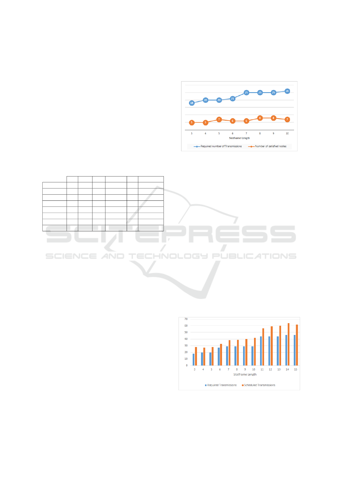
As mentioned in the previous section, when the

network has to satisfy higher data rates the expected

number of transmissions climbs considerably due to

the slotframe length increment and the high packet

rate of nodes. Figure 6 shows an example of this in-

crease in the expected number of transmissions for

the case of a topology consisting of 10 sensor nodes

and a range of slotframes between 3 to 10. The ex-

pected number of transmissions climbs considerably

due to the slotframe length (which basically increases

the time of the slotframe) and the high packet rate of

the nodes. At higher slotframe lengths, the nodes gen-

erate more packets, as a consequence, the associated

number of required transmissions grows accordingly

and the assigned number of slots is not sufﬁcient any-

more.

The ﬁgure also shows the number of satisﬁed

nodes in each slotframe length as the optimization

progresses. The optimization will continue until the

number of transmissions is satisﬁed by all the nodes

in the network, which in this example topology is 10.

We illustrated a portion of the optimization process

only as the solution a slotframe size of 25 or 26 de-

pending on the maximum number of iterations.

Figure 6: Total number of required transmissions in slot-

frame length between 3 and 15 for packet rate higher than 1

packet/sec and the number of satisﬁed nodes.

6.3 Analysis of over Scheduling

The schedule that is created by the optimization al-

gorithm is a conservative schedule with more slots

scheduled than required due to the round up of the

number of required transmissions. The advantage of

over scheduling is that the schedule is less suscepti-

ble to data losses because there are extra time slots

scheduled to accommodate for the re-transmission of

the data. The drawback of over scheduling can be

higher energy consumption as the time slot will con-

sume more energy if scheduled to transit or receive

than if it is in an idle mode.

We calculated the average of the total number of

required transmissions of each node for a network

topology of 10 nodes for different slotframe sizes

ranging from 3 to 15 and compared this to the number

that was scheduled. The results are depicted in Figure

7. The average percentage of overscheduling is 11.6

% for this scenario.

Figure 7: Total number of required transmissions vs. as-

signed number of transmissions for slotframe length be-

tween 3 and 15 for a network consisting of 10 nodes.

TSCH Slotframe Optimization Using Differential Evolution Algorithm for Heterogeneous Sensor Networks

7 CONCLUSION

In this paper we proposed a novel slotframe length

optimization approach using a customized DE opti-

mization algorithm that considers possible packet col-

lisions and interference. It also supports different

packet generation rates. The presented method ﬁnds a

schedule with minimum slotframe length which will

minimize the average delay in the network. The

performance analysis using the TSCH-Sim simulator

conﬁrm that the DE optimized schedule is working

without any collision and interference. We conducted

several experiments using different scenarios to anal-

yse the performance of the algorithm.

As future work, we are planning to include an

adaptive component to the scheduler that can react

to changes in the routes of the network as the cur-

rent static schedule is not ideal as it assumes a static

route. It is also worth investigating how much fur-

ther can the schedule be optimized since the current

approach results in an over-scheduled solution which

can result in scheduled cells that are not being utilized

although it helps to transmit all the packets generated

successfully in case there is a packet loss due to the

unexpected conditions.

REFERENCES

Abu-Khzam, F. N., Bazgan, C., Haddad, J. E., and Sikora,

F. (2015). On the complexity of QoS-aware service

selection problem. In Service-Oriented Computing,

Lecture notes in computer science, pages 345–352.

Springer Berlin Heidelberg, Berlin, Heidelberg.

Elsts, A. (2020). TSCH-Sim: Scaling up simulations of

TSCH and 6TiSCH networks. Sensors, 20(19):5663.

Fafoutis, X., Elsts, A., Oikonomou, G., Piechocki, R., and

Craddock, I. (2018). Adaptive static scheduling in

IEEE 802.15. 4 TSCH networks. In 2018 IEEE 4th

World Forum on Internet of Things (WF-IoT), pages

263–268. IEEE.

Howitt, I. and Gutierrez, J. (2003). IEEE 802.15.4 low rate -

wireless personal area network coexistence issues. In

2003 IEEE Wireless Communications and Network-

ing, 2003. WCNC 2003., volume 3, pages 1481–1486

vol.3.

IEEE Std 802.15.4-2011 (2011). IEEE Standard for

Local and metropolitan area networks–Part 15.4:

Low-Rate Wireless Personal Area Networks (LR-

WPANs). IEEE Std 802.15.4-2011 (Revision of IEEE

Std 802.15.4-2006), pages 1–314.

Javan, N. T., Sabaei, M., and Hakami, V. (2019). IEEE

802.15. 4. E TSCH-based scheduling for throughput

optimization: A combinatorial multi-armed bandit ap-

proach. IEEE Sensors Journal, 20(1):525–537.

Jin, Y., Kulkarni, P., Wilcox, J., and Sooriyabandara, M.

(2016). A centralized scheduling algorithm for IEEE

802.15. 4e TSCH based industrial low power wireless

networks. In 2016 IEEE Wireless Communications

and Networking Conference, pages 1–6. IEEE.

Kharb, S. and Singhrova, A. (2018). Slot-frame length

optimization using hill climbing for energy efﬁ-

cient TSCH network. Procedia Computer Science,

132:541–550.

Khouﬁ, I., Minet, P., and Rmili, B. (2017). Schedul-

ing transmissions with latency constraints in an IEEE

802.15. 4e TSCH network. In 2017 IEEE 86th Vehic-

ular Technology Conference (VTC-Fall), pages 1–7.

IEEE.

Minet, P., Soua, Z., and Khouﬁ, I. (2018). An adaptive

schedule for TSCH networks in the Industry 4.0. In

2018 IFIP/IEEE International Conference on Perfor-

mance Evaluation and Modeling in Wired and Wire-

less Networks (PEMWN), pages 1–6. IEEE.

Ojo, M. and Giordano, S. (2016). An efﬁcient centralized

scheduling algorithm in IEEE 802.15.4e TSCH net-

works. In 2016 IEEE Conference on Standards for

Communications and Networking (CSCN). IEEE.

Palattella, M. R., Accettura, N., Dohler, M., Grieco,

L. A., and Boggia, G. (2012). Trafﬁc aware schedul-

ing algorithm for reliable low-power multi-hop ieee

802.15. 4e networks. In 2012 IEEE 23rd International

Symposium on Personal, Indoor and Mobile Radio

Communications-(PIMRC), pages 327–332. IEEE.

Soua, R., Minet, P., and Livolant, E. (2016). Wave: a dis-

tributed scheduling algorithm for convergecast in ieee

802.15. 4e tsch networks. Transactions on Emerging

Telecommunications Technologies, 27(4):557–575.

Storn, R. and Price, K. P. (1997). Differential evolution a

simple and efﬁcient adaptive scheme for global opti-

mization over continu. Journal of Global Optimiza-

tion.

Teles Hermeto, R., Gallais, A., and Theoleyre, F. (2017).

Scheduling for IEEE802.15.4-TSCH and slow chan-

nel hopping MAC in low power industrial wireless

networks: A survey. Computer Communications,

114:84–105.

Urke, A. R., Kure, Ø., and Øvsthus, K. (2021). A survey of

802.15.4 TSCH schedulers for a standardized indus-

trial internet of things. Sensors, 22(1):15.

Vatankhah, A. and Liscano, R. (2022). Differential evolu-

tion optimization of TSCH scheduling for heteroge-

neous sensor networks. In 2022 IEEE Wireless Com-

munications and Networking Conference (WCNC),

pages 1491–1496.

Watteyne, T., Handziski, V., Vilajosana, X., Duquennoy, S.,

Hahm, O., Baccelli, E., and Wolisz, A. (2016). In-

dustrial Wireless IP-Based Cyber –Physical Systems.

Proceedings of the IEEE, 104(5):1025–1038.

SENSORNETS 2023 - 12th International Conference on Sensor Networks