Local Reﬂectional Symmetry Detection in Point Clouds Using a Simple

PCA-Based Shape Descriptor

Luk

s Hruda

1 a

, Ivana Kolingerov

1 b

and David Podgorelec

2 c

Department of Computer Science and Engineering, Faculty of Applied Sciences, University of West Bohemia,

Univerzitn

ı 8, 301 00 Plze

n, Czech Republic

Faculty of Electrical Engineering and Computer Science, University of Maribor, Koro

ska cesta 46, 2000 Maribor, Slovenia

Keywords:

Symmetry, Local, Reﬂectional, PCA, Descriptor.

Abstract:

Symmetry is a commonly occurring feature in real world objects and its knowledge can be useful in various

applications. Different types of symmetries exist but we only consider the reﬂectional symmetry which is

probably the most common one. Multiple methods exist that aim to ﬁnd the global reﬂectional symmetry of

a given 3D object and although this task on its own is not easy, ﬁnding symmetries of objects that are merely

parts of larger scenes is much more difﬁcult. Such symmetries are often called local symmetries and they

commonly occur in real world 3D scans of whole scenes or larger areas. In this paper we propose a simple

PCA-based local shape descriptor that can be easily used for potential symmetric point matching in 3D point

clouds and, building on previous work, we present a new method for detecting local reﬂectional symmetries in

3D point clouds which combines the PCA descriptor point matching with the density peak location algorithm.

We show the results of our method for several real 3D scanned scenes and demonstrate its computational

efﬁciency and robustness to noise.

1 INTRODUCTION AND

RELATED WORK

Many objects in real world contain some form of

symmetry. By symmetry we understand a geometric

transformation that leaves a given object unchanged

excluding identity. Having a 3D object X a transfor-

mation T ̸= I is a symmetry of X if T (X) = X, i.e.

when after T is applied on X each point of the trans-

formed X ends up in any point of the original X . There

are different types of symmetry according to which

types of transformations are considered. In this pa-

per we only consider reﬂectional symmetry where the

transform T is a reﬂection over a plane and can be

represented by the reﬂection plane itself - the sym-

metry plane. Also, in reality, there is never a perfect

symmetry which means that we are ultimately inter-

ested in approximate reﬂectional symmetries where

the transform does not match the object onto intself

perfectly but only approximately. The term approx-

imate symmetry, however, does not seem to have an

https://orcid.org/0000-0002-9477-7464

https://orcid.org/0000-0003-4556-2771

https://orcid.org/0000-0002-0701-9201

exact formal deﬁnition.

The knowledge of symmetry has various appli-

cations, mostly in computer vision, such as incom-

plete object reconstruction (Sipiran et al., 2014), ob-

ject alignment (Li et al., 2016) or symmetrical editing

(Martinet et al., 2006). But before any application is

possible the symmetries ﬁrst need to be found.

The ﬁeld of symmetry detection has advanced a

lot in the past decades providing numerous methods

that aim to ﬁnd the symmetry plane(s) of a given in-

put object. Such a task is difﬁcult on its own but es-

pecially the modern methods are able to provide a ro-

bust, reliable and fast solutions that are often capable

of ﬁnding visually plausible symmetry planes in ob-

jects with very weak reﬂectional symmetries or with

missing geometry (like those in Fig. 2), they can work

with various types of data and can often solve the task

at hand in matters of seconds, sometimes even hun-

dreds or tens of milliseconds. Examples of such meth-

ods are (Martinet et al., 2006; Comb

es et al., 2008;

Sipiran et al., 2014; Li et al., 2016; Nagar and Raman,

2020; Hruda et al., 2022;

Zalik et al., 2022). Still, like

in most ﬁelds, there is room for further improvements

since even the most advanced methods cannot handle

everything.

Hruda, L., Kolingerová, I. and Podgorelec, D.

Local Reﬂectional Symmetry Detection in Point Clouds Using a Simple PCA-Based Shape Descriptor.

DOI: 10.5220/0011622200003417

In Proceedings of the 18th International Joint Conference on Computer Vision, Imaging and Computer Graphics Theory and Applications (VISIGRAPP 2023) - Volume 1: GRAPP, pages

52-63

ISBN: 978-989-758-634-7; ISSN: 2184-4321

 2023 by SCITEPRESS – Science and Technology Publications, Lda. Under CC license (CC BY-NC-ND 4.0)

Figure 1: Examples of scenes that exhibit one or more reﬂectional symmetries in their subparts - local symmetries (data

source: (Funk et al., 2017)).

Figure 2: Examples of weakly symmetrical objects with

plausible symmetry planes marked by the red line (source:

(Hruda et al., 2022)).

However, in this case the task is somewhat simpli-

ﬁed by the fact that the whole object is anticipated to

be symmetric and the methods aim to ﬁnd the plane

that best captures its symmetry. The problem be-

comes remarkably more difﬁcult when the input ob-

ject or scene is not globally symmetric but merely

contains some noticeably symmetric area as its sub-

part. This is often referred to as local symmetry and

it is quite common in real 3D scans where the sym-

metric object is often surrounded by other geome-

try or sits on a larger ﬂat surface that represents the

ﬂoor/ground (see Fig. 1 for speciﬁc examples). There

can also be multiple symmetric objects in the scene.

The methods that aim to solve this type of problem

are not as plentiful and those that exist often require

some form of pre-segmentation (Ecins et al., 2017),

use a local shape descriptor that requires a mesh on

the input (often a manifold one) (Mitra et al., 2006;

Shi et al., 2016) or seem to be very slow even for

scenes with a rather low point count (Lipman et al.,

2010).

In this paper we propose a very simple PCA-

based local shape descriptor and we present a new

method for ﬁnding local reﬂectional symmetries in

point clouds that uses this descriptor for point match-

ing. Our work builds on the previous work of (Mitra

et al., 2006), (Hruda et al., 2019) and (Hruda et al.,

2022).

2 METHOD DESCRPTION

Let X = {x

, x

, ..., x

}, x

∈ E

be a set of 3D points

(point cloud) that represents the input scene and let

r(P, x) be a transformation that represents an arbitrary

point x ∈ E

reﬂected over a given plane P. The goal

of our method is to extract local reﬂectional symme-

tries from X, i.e. a set of planes {P

, P

, ..., P

} where

each plane P

represents a reﬂectional symmetry de-

scribed by a transformation r(P

, x).

We represent a general plane P by its implicit

equation ax + by + cz + d = 0 with a, b, c, d being the

plane coefﬁcients. We consider all planes to always

have unit normals, i.e. ||[a, b, c]

|| = 1. We further

denote r

vec

(P, v) a function that represents a general

vector v ∈ E

reﬂected over a given plane P where

v is a direction without position. The function r

vec

is computed in the same way as r only ignoring the

plane position, i.e. as if d = 0.

2.1 PCA-Based Shape Descriptor

Various symmetry detection methods use local shape

descriptors to ﬁnd potentially symmetric pairs of

points throughout the input object/scene, e.g. (Mitra

et al., 2006; Shi et al., 2016; Sipiran et al., 2014). In

most cases, these descriptors are curvature/Laplacian-

based and are generally difﬁcult to compute on point

clouds or even non-manifold meshes because robust

estimation of the principal curvatures or the Laplacian

mostly requires connectivity information and mani-

fold surface.

In contrast, we use a very simple local shape de-

scriptor based on the Principal Component Analysis

(PCA) (Wold et al., 1987) that can be computed on a

general set of points (i.e. requires neither connectivity

nor manifoldness) and we show that it can be used for

symmetric point matching as well. The descriptor is

computed as follows.

Let us take an arbitrary point x ∈ E

(not nec-

Local Reﬂectional Symmetry Detection in Point Clouds Using a Simple PCA-Based Shape Descriptor

essarily contained in X ) and select a radius r. The

set of points N

= {x

: x

∈ X, ||x

− x|| ≤ r} is de-

ﬁned to be the neighborhood of the point x. By

computing the PCA for the points in N

we get the

three orthogonal eigenvectors v

x,1

, v

x,2

, v

x,3

, ||v

x,i

|| =

1, that correspond to the principle directions of N

and three eigenvalues λ

x,1

, λ

x,2

, λ

x,3

where each λ

x,i

corresponds to the variance of N

in the direction

of v

x,i

. The eigenvectors and eigenvalues are in-

dexed in such a way that |λ

x,1

| ≥ |λ

x,2

| ≥ |λ

x,3

| which

means that v

x,1

always represents the direction with

the largest variance. The PCA-based shape descrip-

tor for point x can then be simply described by

the eigenvectors v

x,1

, v

x,2

, v

x,3

and by a vector λ

[

|λ

x,1

norm

|λ

x,2

norm

|λ

x,3

norm

]

where λ

norm

is a normalization

constant set so that it equals the variance of all points

lying on a line segment of length 2r which is the

maximum distance of any two points in any neigh-

borhood. This way λ

norm

simulates an eigenvalue for

points distributed uniformly across the entire neigh-

borhood in the direction of a corresponding eigenvec-

tor. The variance of a discrete set of k 1-dimensional

points x

, x

, ..., x

∑

i=1

(µ − x

)

where µ is the

mean of the points. For a continuous case of a line

segment of length 2r we can take the interval ⟨−r, r⟩

and compute its variance by integration. The mean of

the interval is zero so we get

norm

−r

(0 − x)

dx =

Given r is chosen relative to the input scene size,

the normalization makes λ

independent of the scene

scale.

The vector λ

holds information about the shape

of the neighborhood that is invariant under both rota-

tion and translation. This means that for two different

points x, y, if λ

and λ

are similar there is a good

chance that the points in the two neighborhoods N

represent similar shapes just differently positioned

and oriented which in turn implies that there could be

symmetry between them. The λ

vector values can

also be easily visualized as shown in Fig. 3 where

each point x of the scene is assigned a color whith

RGB values corresponding respectively to the coordi-

nates of λ

computed with r =

avrg

where l

avrg

is the

average distance of the points in the scene from the

scene’s centroid. It can be seen that the symmetric

counterparts of the couch in the middle are very sim-

ilarly colored, i.e. the λ

λ vectors in them are similar.

However, the similarity of λ

and λ

does not im-

ply in any way that the potential symmetry between

and N

is reﬂectional. This information can be

derived from the eigenvectors v

x,i

and v

y,i

, i = 1, 2, 3.

Speciﬁcally, having a general plane P, if the neighbor-

Figure 3: A scene with a reﬂecionally symmetric couch in

the middle colored using the eigenvalues of the PCA de-

scriptor as RGB values (data source: (Funk et al., 2017)).

hood N

is reﬂectionally symmetric with the neigh-

borhood N

w.r.t. the plane P then each eigenvector

x,i

will be the same as or opposite to r

vec

(P, v

y,i

These properties of the PCA descriptor can be

used to ﬁnd potentially symmetric pairs of points as

will be described in the following text. Note that the

descriptor can also be computed for points that are not

directly contained in the input point cloud X , this will

be shown useful later.

2.2 Descriptor Computation

To start matching potentially symmetric neighbour-

hoods using the PCA descriptor it ﬁrst needs to be

computed but doing so for all points in the input scene

X could easily get computationally overwhelming as

real 3D scanned scenes often consist of hundreds of

thousands of points. Also, when computing the de-

scriptor for a given point, the points in the neighbour-

hood of the selected radius ﬁrst need to be extracted

and doing so while avoiding brute-force computation

is more than desirable.

2.2.1 Simpliﬁcation

Instead of computing the descriptor for all points of

the input scene X we create a simpliﬁed version of

the scene denoted X

′

= {x

′

, x

′

, ..., x

′

}, x

′

∈ E

. We

use the same grid-based point cloud simpliﬁcation al-

gorithm as used in (Hruda et al., 2022) which stems

from putting the points of the point cloud into cells

of a uniform grid and averaging points in every cell.

Therefore, each cell provides a single point of the

new point cloud which is generally not contained in

the original point cloud. The process is repeated sev-

eral times with decreasing cell size until a target point

count is reached approximately. We use this algo-

rithm with target point count 10, 000 which is then

the rough number of points of X

′

GRAPP 2023 - 18th International Conference on Computer Graphics Theory and Applications

Since the PCA descriptor can be computed for

points outside of X but still represent its local features

we compute it at the m (roughly 10, 000) points of X

′

but for its computation at a given point x

′

∈ X

′

use the neighbourhood extracted from X in the cor-

responding region. This not only reduces computa-

tional cost but also ensures that the points used for

symmetric matching (see Section 2.4) are more uni-

formly distributed over the scene.

2.2.2 Neighbourhood Extraction

To efﬁciently extract points of X lying in a given

neighbourhood of radius r we again use a grid-based

approach from (Hruda et al., 2022). At the beginning

the points of X are stored in a uniform grid with cell

size r ×r ×r. Then, when a neighbourhood of a given

point x

′

needs to be extracted, we search for points

whose distance from x

′

is ≤ r only among points that

are in the same cell as x

′

and cells adjacent to this cell.

This is, of course, signiﬁcantly faster than brute-force

iterating over all points of X, at least when r is rea-

sonably small. We use r =

avrg

as the default value

where the number 5 was chosen experimentally.

Other data structures, such as K-d tree, BSP tree

or octree, could be used as well. However, we believe

that the grid-based approach provides similar boost

in performance and is simpler to implement than the

tree-based structures.

2.3 Finding Planar Points

The PCA descriptor at points that lie in roughly pla-

nar neighbourhoods (ﬂoor, walls, etc.) does not re-

ally provide useful information in terms of symmetry.

First, because the ﬁrst two eigenvectors have basically

random direction at planar points. Second, because

planar areas are usually quite plentiful in real world

scenes and could easily cause too many false positive

symmetric matches - this can be easily seen in Fig.

3 where the planar points are colored yellow. This

is why we ﬁrst detect the points of X

′

that have ap-

proximately planar neighbourhoods so that we could

exclude them from the later steps.

For a given point x

′

∈ X

′

we decide whether it is

planar in the following way. We construct a plane that

passes through x

′

and whose normal vector is given

by v

′

×v

′

. We then compute the average distance

of points in N

′

from this plane and denote it ∆

⊥

′

this value will be the smaller the points in N

′

ﬁt the

plane. We also project each point in N

′

orthogonally

on the same plane and compute the average distance

of these projected points from x

′

. We denote it ∆

∥

′

and it serves as a normalization value. Now the point

′

is marked as planar if

∆

⊥

′

∆

∥

′

< ε

∆

where ε

∆

= 0.1 and

its value was experimentally chosen.

2.4 Symmetric Point Matching

After the PCA descriptor has been computed in all

points of the simpliﬁed point cloud X

′

and planar

points were found we start searching for potentially

symmetric neighbourhoods. First, we ﬁnd pairs of

non-planar points with similar λ

λ vectors and then we

verify their potential reﬂectional symmetry using the

PCA eigenvectors.

2.4.1 λ

λ Similarity Matching

For every non-planar point x

′

∈ X

′

, i = 1, ..., m we ﬁnd

a non-planar point x

′

∈ X

′

, j = 1, ..., m, i ̸= j such

that ||λ

′

−λ

′

|| ≤ ε

, where ε

= 0.05, and we add

the pair (x

′

, x

′

) to a set Q of potentially symmetric

point pairs. If there are multiple points x

′

satisfying

these conditions we only use the one with the smallest

distance ||λ

′

−λ

′

||. To avoid brute-force computa-

tion we again use the grid-based approach described

in Section 2.2.2, only this time we store the λ

λ vec-

tors in the grid with cell size ε

× ε

, and use it

to efﬁciently ﬁnd other vectors up to the distance ε

from a given λ

λ vector. The value of ε

was chosen

experimentally.

In the end the set Q contains pairs (x

′

, x

′

) where

each such pair of points could potentially provide ev-

idence for symmetry.

2.4.2 Symmetry Veriﬁcation

For each of the pairs acquired in the previous step we

need to check whether it truly presents evidence of

potential reﬂectional symmetry. This is done using

the eigenvectors of the PCA descriptor as suggested

in Section 2.1.

Since the ﬁrst eigenvector bears the most relevant

information about the shape of the local neighbor-

hood (it corresponds to the largest eigenvalue), for

simplicity, we do not use the second and third eigen-

vectors for the symmetry veriﬁcation, only the ﬁrst

one. Therefore, we denote v

′

= v

′

the relevant

eigenvector of the PCA descriptor computed at point

′

. However, both the second and third eigenvectors

could be included in the veriﬁcation step but our ex-

periments do not suggest that it would cause a signif-

icant improvement.

For each one of the point pairs (x

′

, x

′

) ∈ Q we con-

struct a plane P such that r(P, x

′

) = x

′

and perform a

Local Reﬂectional Symmetry Detection in Point Clouds Using a Simple PCA-Based Shape Descriptor

Figure 4: A scene with the PCA-based descriptor symmetric matching - the symmetrically matched pairs of points of X

′

are

connected by the black lines, the coloring corresponds to the descriptor eigenvalues computed on X

′

, the grey color indicates

planar areas.

simple test. The pair of points is accepted as poten-

tially reﬂectionally symmetric if

min(||r

vec

(P, v

′

) − v

′

||, ||r

vec

(P, v

′

) + v

′

||) ≤ ε

where ε

= 0.1 and its value was chosen based on vast

experiments. When the pair of points passes the test

the plane P is added to a set C. As a result we ac-

quire a set C = {P

, P

, ..., P

} of candidate symmetry

planes.

Fig. 4 shows the symmetric matching for the

scene with the couch in the middle. The black lines

connect pairs of points of X

′

that were matched to-

gether and passed the veriﬁcation step, i.e. their sym-

metry plane is in C. The coloring now reﬂects eigen-

values of the PCA descriptor computed for X

′

- the

color of a given point of X

′

was transferred to all

points of the input scene X that were in the same cell

of the simpliﬁcation grid in the last iteration of the

simpliﬁcation process (see Section 2.2.1). The grey

colored areas correspond to points that were marked

as planar (see Section 2.3). Among others, the ﬁgure

reveals numerous symmetric matches between the re-

ﬂectionally symmetric counterparts of the couch indi-

cating that there are many planes in C that capture its

symmetry.

2.5 Mode Seeking

We follow the theory, used e.g. in (Mitra et al., 2006;

Shi et al., 2016; Hruda et al., 2019), that the sig-

niﬁcant symmetries should now form modes in the

space of candidate transformations - planes in our

case. Finding the modes is often solved by clustering

(Mitra et al., 2006; Shi et al., 2016) but we believe

that clustering algorithms might become unnecessar-

ily complex and computationally expensive. Also, a

cluster of points might not necessarily correspond to

a local mode since a mode is represented by a sin-

gle point but a cluster is a set of points. Therefore,

with clustering, there would be some further actions

required regarding selecting a proper point from each

cluster to represent the mode.

Instead, we use the density peak location algo-

rithm proposed in (Hruda et al., 2019) modiﬁed to

serve our purpose. In general, the algorithm can be

described as follows. Let ρ(P

) be the density at a

given candidate P

∈ C. The density at a given point

in the space of planes corresponds to how many simi-

lar candidates there are to this point, i.e. the points

of high density should correspond to the modes in

the candidate space. The most signiﬁcant mode, and

therefore the strongest symmetry candidate, would be

simply identiﬁed as argmax

∈C

ρ(P

2.5.1 Density Function

The density function is deﬁned as

ρ(P

) =

∑

∈C

K(D(P

, P

))

where D(P

, P

) is a distance measure between P

and

and K(l) is a kernel which in (Hruda et al., 2019)

was originally set to the standard Gaussian function

but we instead use the modiﬁed Wendland’s function

from (Hruda et al., 2022). We denote it ϕ(x), it has a

very similar shape to the Gaussian function but is lo-

cally supported and smoothly goes to 0 at x = 2.6.

We set K(l) = ϕ(αl) where α is a spread parame-

ter and l represents distance. We experimentally set

α as α = 25. The local support property of the ker-

nel draws a direct boundary between candidates that

contributed to the density of P

and those that did not

which will be used later.

Denoting p

= [a

, b

, c

avrg

]

a representative co-

efﬁcient vector of candidate plane P

, the distance

GRAPP 2023 - 18th International Conference on Computer Graphics Theory and Applications

(a) P

(b) Initial Sym(P

) (c) Area(P

)

Figure 5: A plane P

(the black rectangle) detected by the density peak location algorithm - (a), the initial set Sym(P

) - (b),

the ﬁnal symmetric subpart of X, Area(P

) (marked by the green color) - (c).

measure D is deﬁned as

D(P

, P

) = min(||p

− p

||, ||p

+ p

|||) (1)

which, according to (Hruda et al., 2020), is usable for

this purpose but only when the input object is cen-

tered at the origin which is why, at the beginning, we

translate the input scene X such that its centroid lies

at the origin and at the end we translate the detected

symmetry planes back. The division of the d coefﬁ-

cient by l

avrg

ensures its normalization by the scene

size which, according to (Hruda et al., 2020), is also

required for the distance measure to be meaningful.

2.5.2 Density Peak Location

In (Hruda et al., 2019) the density peak location al-

gorithm was only used to ﬁnd the most signiﬁcant

mode in the transformation space and, due to usage

of a non-Euclidean distance metric, the Vantage Point

Tree (Yianilos, 1993) data structure was used for ef-

ﬁcient computation of the density function. However,

we can have multiple symmetries in a single scene

which means we should be able to ﬁnd multiple lo-

cal modes, not just the largest one. Since our distance

function D is Euclidean, when computing the density

for a candidate P

, we can use any standard data struc-

ture to quickly ﬁnd only the candidates whose dis-

tance from P

is not larger than the radius of the sup-

port region of the kernel K. We again use a grid as

the auxiliary data structure, only this time in 4 dimen-

sions, as previously used in (Hruda et al., 2022) for

ﬁnding similar planes.

We ﬁrst ﬁnd the candidate P

∈ C that maximizes

the density function ρ(P

) and add it to a set S of pre-

liminary symmetries. Then, we remove from C all

candidates that had non-zero contribution to the den-

sity in P

, i.e. were inside the support region of the

kernel K at P

. We can now repeat this process to ﬁnd

the second most signiﬁcant mode etc. We can either

do this a certain predeﬁned number of times or, as we

do, keep repeating the process as long as the density

at each newly located mode is above a given thresh-

old. We keep ﬁnding new modes and adding them to

S as long as their density value is at least half of the

density that the ﬁrst located mode had. At the end the

set S ⊂ C contains the preliminary reﬂectional sym-

metries.

2.6 Finalizing Symmetries

The planes in the set S extracted in the previous step

might not be accurate and not all of them actually rep-

resent plausible symmetries. For each plane in S we

now need to extract the subpart of X which is actually

symmetric w.r.t. the plane and reﬁne the symmetry for

the corresponding subpart. At last, we need to discard

symmetries that are too weak to be meaningful.

2.6.1 Extracting Symmetric Areas

For each of the planes in S we ﬁnd the symmetric sub-

part of X in the following way. For a given plane

∈ S we take all the planes that contributed by a

non-zero value to its density in the density peak lo-

cation step in which it was added to S (see Section

2.5.2). For each of these contributing planes we take

the pair of points that initially created the plane (see

Sections 2.4.1 and 2.4.2) and add them to a set de-

noted Sym(P

) - a set of points of X

′

that contributed

to locating P

as a mode in the candidate space. The

points in Sym(P

) provide a rough information about

the position and size of the subpart of X that is sym-

metric w.r.t. P

. Fig. 5a shows an example of a plane

(the black rectangle) found by the density peak lo-

cation process and Fig. 5b shows the points in the

corresponding Sym(P

) set.

We compute the centroid of Sym(P

) and use PCA

to compute its principal axes - PCA eigenvectors v

, v

- and the variance in the direction of each of

these axes - eigenvalues λ

, λ

. We express each

point x

∈ Sym(P

) as a point in the local coordinate

system with the origin at the centroid of Sym(P

) and

basis directions of v

, v

. This local expression

of point x

is denoted

= [ˆx

, ˆy

, ˆz

]

. We consider

a point

an outlier if the absolute value of one of

Local Reﬂectional Symmetry Detection in Point Clouds Using a Simple PCA-Based Shape Descriptor

its coordinates is larger than double of the standard

deviation of the points of Sym(P

) (its square is larger

than quadruple of the variance) in the corresponding

direction, i.e. we only keep points x

for which the

expression

ˆx

≤ 4λ

and ˆy

≤ 4λ

and ˆz

≤ 4λ

(2)

is true and remove all other points from Sym(P

). We

repeat this process one more time (compute centroid

and PCA of the new Sym(P

) and remove outliers) and

then we create a point set Area(P

) ⊂ X that contains

all points from the input point cloud X that satisfy the

expression in Eq. (2) only this time with x

∈ X and

the centroid, principal axes and variances being com-

puted for the ﬁnal Sym(P

) point set. The set Area(P

)

is now considered the subpart of X that is symmetric

w.r.t. the preliminary symmetry plane P

∈ S. Fig. 5c

depicts the extracted Area(P

) (colored green) for the

plane from Fig. 5a.

2.6.2 Symmetry Reﬁnement

We now reﬁne the preliminary symmetries with re-

spect to their corresponding subparts of the input

point cloud X. For each plane P

∈ S we use the op-

timization step for global reﬂectional symmetry from

the method of (Hruda et al., 2022) where P

is the ini-

tial plane and Area(P

) is the expected globally sym-

metric object. This method uses a differentiable sym-

metry measure that represents the symmetry of the in-

put object w.r.t. the given plane and a gradient-based

optimization to ﬁnd its local maximum. We also in-

clude the simpliﬁcation process described in Section

3.3 in (Hruda et al., 2022) where the input object is

simpliﬁed to roughly 1000 points before the optimiza-

tion is started.

We replace each plane P

∈ S by a plane that was

converged to by the optimization started from P

Area(P

). As a result the accuracy of the symmetry

planes in S should increase.

2.6.3 Excluding Bad Symmetries

The density peak location in the space of candidate

planes created by the PCA-based descriptor point

pairing can produce false positives and even the re-

ﬁnement from the previous step does not guarantee

that all the planes in S are meaningful.

We use the symmetry measure from the reﬁne-

ment step to determine the plausibility of a given

plane. The symmetry measure is computed by trans-

forming each point of the object by the given trans-

form (in our case reﬂection over a plane) and comput-

ing similarity (in terms of distance) of the transformed

point to all points of the object. All the similarities

are summed together to provide the measure value

(for more details we refer to (Hruda et al., 2022)).

The problem is that this value is not normalized in

any way and does not only depend on the strength of

the symmetry but also on various properties of the in-

put object. Therefore, we use a modiﬁed version of

the symmetry measure where we divide its value by

a symmetry measure value that would be achieved by

perfect symmetry. We simulate the perfect symme-

try measure by computing the symmetry measure of

the identity transform. We call this modiﬁed version

Relative Symmetry Measure (RSM).

For each plane P

∈ S we now compute the RSM

of the reﬂection over P

transform on Area(P

). All

planes with RMS greater than 0.4 are accepted as the

resulting symmetry planes of the input scene X.

3 RESULTS

Our method was implemented in C# and the results

were acquired on a computer with CPU Intel® Core

i7-10700F (frequency: 2.9GHz, turbo boost: 4.8GHz,

8 cores, L1 cache: 512kB, L2 cache: 2MB, L3 cache:

16MB) and 32GB memory (frequency: 3.2GHz) run-

ning a Windows 10 operating system.

We tested the method on several real 3D scenes

from the dataset (Funk et al., 2017). The results can

be seen in Fig. 6, the black rectangles indicate the

detected planes. We note that although the objects in

the ﬁgure are represented by triangle meshes, we only

used the vertices as the input point cloud X for our

method. Triangle meshes are much easier to visualize

and most likely the objects were originally scanned

as point clouds and meshing was done in post pro-

cessing which means that the vertices we use actually

represent the original raw point clouds. It seems that

the strongest symmetries are detected correctly in all

of these 12 scenes but is should be noted that some

of the scenes also contain some weaker symmetries

that were not identiﬁed by our method, this is espe-

cially noticeable in Scene 12. On the other hand, the

method sometimes ﬁnds symmetries that are techni-

cally correct but would not be expected by a human

observer. An example of this case is Scene 7 where

two symmetries were found on the long edge of the

couch seat on the right side. Such symmetries are not

meaningful for a person but it is understandable that

the method detects them since there are many points

symmetric w.r.t. both these planes. In Scene 9 our

method also identiﬁed a plausible symmetry plane of

the partial chair/couch in the top right corner. Some-

times, mostly when there are multiple objects in dif-

ferent places that are symmetric w.r.t. the same plane,

GRAPP 2023 - 18th International Conference on Computer Graphics Theory and Applications

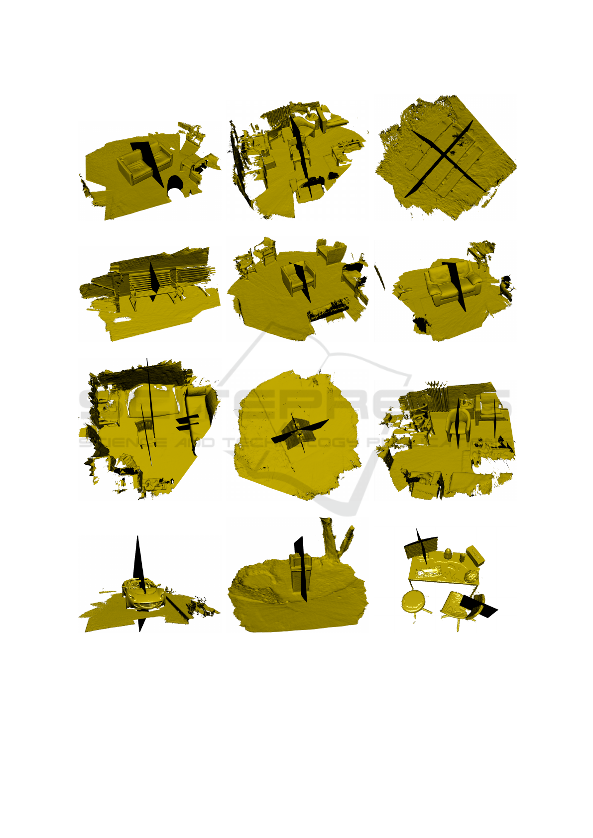
(a) Scene 1 (b) Scene 2 (c) Scene 3

(d) Scene 4 (e) Scene 5 (f) Scene 6

(g) Scene 7 (h) Scene 8 (i) Scene 9

(j) Scene 10 (k) Scene 11 (l) Scene 12

Figure 6: The results of our method on several 3D scanned scenes from the (Funk et al., 2017) dataset, the detected symmetry

planes are marked by the black rectangles.

the method covers a larger area with a single sym-

metry. This can be seen in Scene 2 where we have

a single symmetry plane for the chair in the middle

and the partial chair in front of it because both these

objects were included in a single symmetric area.

For demonstration of the quality of the detected

Local Reﬂectional Symmetry Detection in Point Clouds Using a Simple PCA-Based Shape Descriptor

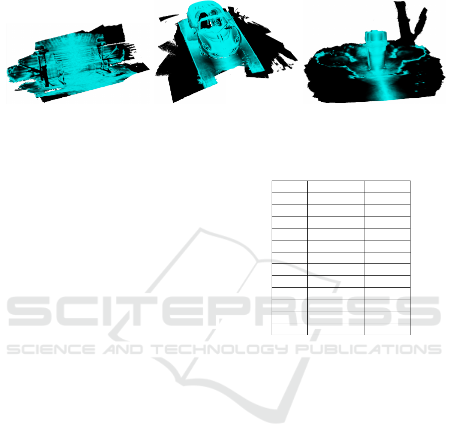
(a) Scene 4 (b) Scene 10 (c) Scene 11

Figure 7: Symmetry coloring from (Hruda et al., 2022) for the one detected plane in three different scenes - the lighter the

color the stronger the symmetry of the given point.

symmetries we used the symmetry coloring proposed

in (Hruda et al., 2022) to show how strong a given

symmetry is for different points of the scene. We used

this for scenes 4, 10 and 11 where we always took the

one detected plane (see Fig. 6) and we colored all

the points in the input scene in correspondence to the

symmetry of this plane. The coloring is depicted in

Fig. 7. The lighter the color the stronger the symme-

try of the given point. The symmetry mostly covers

the object for which it was detected but, of course,

partially also includes some other regions of the scene

such as the ground.

Tab. 1 shows the number of points and computa-

tion time of our method for each scene. Although the

point counts of the scenes are quite large (hundreds of

thousands) the computation time ranges around 20s,

and sometimes gets under 10s, which can be consid-

ered rather fast. The exception is Scene 10 which has

almost 2 million points. We use a single-threaded im-

plementation of the method but its most time consum-

ing stages (descriptor computation and point pairing)

could be easily parallelized which would make the

overall method potentially several times faster.

Our method should work on point clouds with

even larger point counts (tens of millions / billions)

but the computational cost would probably become

overwhelming.

3.1 Noisy Data

In order to test robustness to noise of our method and

the PCA-based descriptor we selected two scenes and

added a vector [rand

, rand

]

· l

avrg

· mag to

each of their points where rand

, rand

are uni-

form random values from −1 to 1 and mag is the noise

magnitude. Fig. 9 shows the detected planes for the

two scenes with added noise with mag = 0.025 and

mag = 0.05. We colored the objects in the same way

as in Fig. 4 to show what effect the noise has on the

λ vectors of the PCA descriptor. The detected sym-

metry planes are very similar to those detected on the

Table 1: The computation time of our method in seconds

for each one of the scenes from Fig. 6.

Scene Point count Time [s]

1 387540 12.3

2 598324 18

3 439089 12.5

4 287875 8.6

5 515496 18.7

6 380592 10.5

7 559905 24.4

8 321052 10.6

9 566153 16.1

10 1891185 133.7

11 288759 9.3

12 233600 7.7

noiseless versions of the scenes and the λ

λ vectors of

the descriptor seem to still well represent similarities

of the local neighborhoods that could be symmetric.

The planar area detection step seems to start fail-

ing under the inﬂuence of the noise but it apparently

does not impact the symmetry detection results very

much. This might partially be because the noise also

makes the PCA eigenvectors a little more random in

the planar regions which probably also lowers the po-

tential for false positive matches.

Note that, although the ﬁrst step of our method

is simpliﬁcation which partially suppresses the noise,

the simpliﬁed point set is only used for point pair-

ing but the PCA-based descriptor is computed for the

points of the original point set and is therefore fully

affected by the noise.

Fig. 8 shows how the noise changes the detected

plane for different scenes. For this experiment we

only used scenes where the method ﬁnds exactly one

symmetry plane. For each scene we kept increas-

ing the noise magnitude and for each magnitude level

we used the density peak location algorithm to ﬁnd

the single most pronounced plane in the candidate

space regardless of its RSM value. We then used

the plane distance function from Eq. (1) to measure

GRAPP 2023 - 18th International Conference on Computer Graphics Theory and Applications

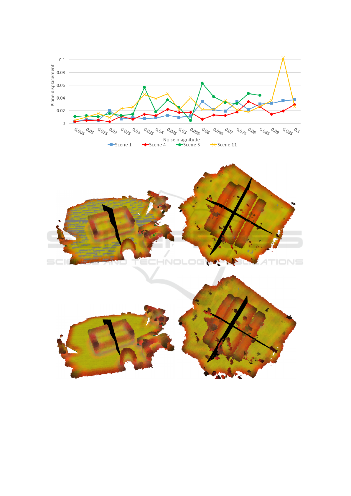
Figure 8: Displacement of the symmetry plane detected on different scenes with different magnitude of added noise from the

plane detected on the noise free version of the scene expressed in terms of the distance function from Eq. (1).

(a) Scene 1, mag = 0.025 (b) Scene 3, mag = 0.025

Figure 9: Results of our method for two different scenes with added noise with mag = 0.025 and 0.05, the colors indicate

eigenvalues of the PCA descriptor, grey corresponds to detected planar areas.

the displacement of the detected plane from the plane

that was found on the original noise free scene. For

Scenes 1 and 4 there seems to be roughly linear de-

pendency between the noise magnitude and the plane

Local Reﬂectional Symmetry Detection in Point Clouds Using a Simple PCA-Based Shape Descriptor

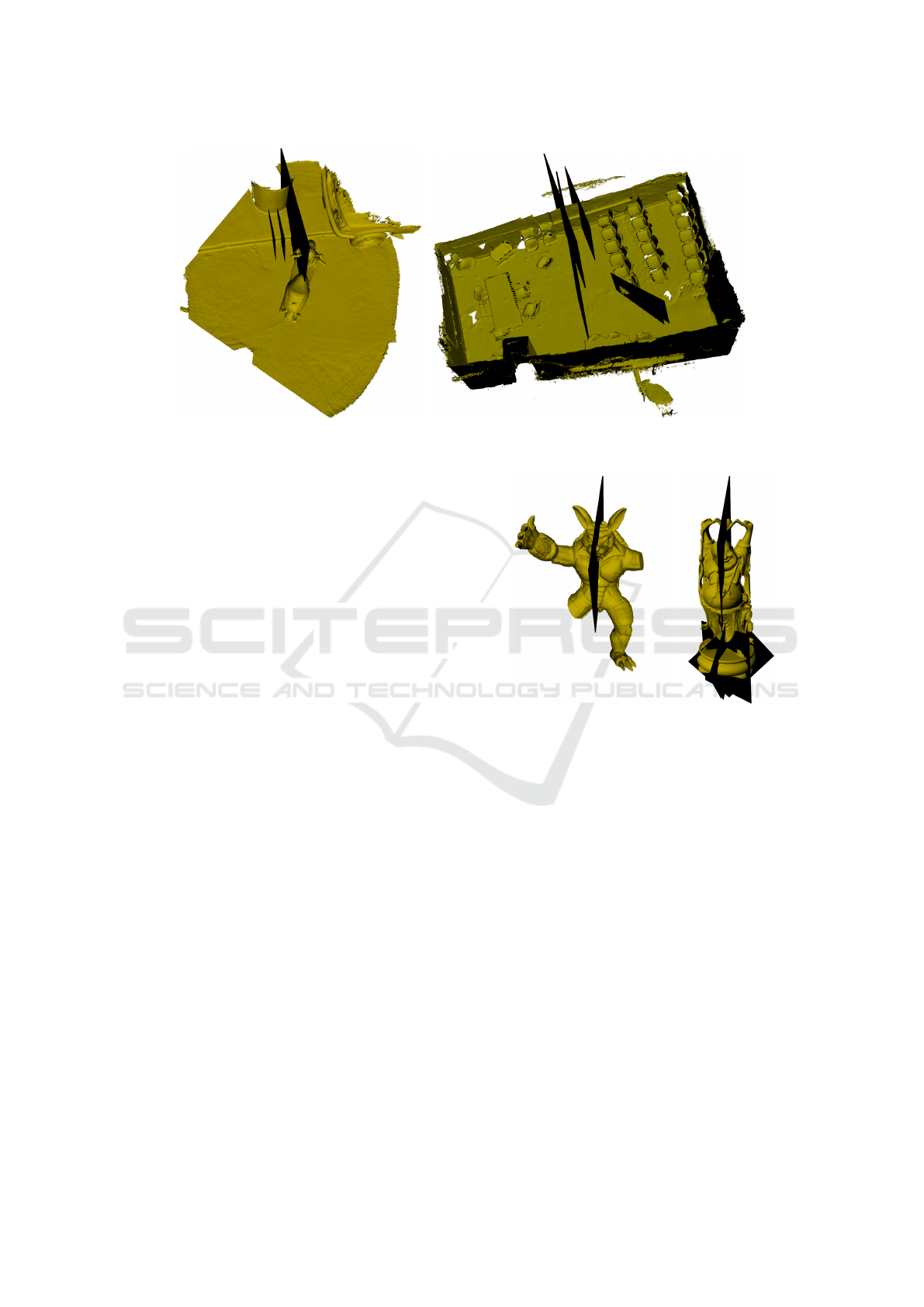
(a) Fail 1 (b) Fail 2

Figure 10: Examples of two input scenes where the method fails to detect plausible symmetry planes.

displacement which increases rather slowly showing

that the noise does not inﬂuence the function of the

PCA descriptor and the density peak location step

signiﬁcantly. In Scenes 5 and 11 the displacement

appears to be much more random and oscillates a

lot. For Scene 5 we do not include the displacement

for mag > 0.085 because for larger magnitudes the

method stops detecting the corresponding plane com-

pletely and the displacement increases by an order of

magnitude which would make the graph unreadable.

3.2 Globally Symmetric Objects

Since a method designed to detect local symmetries

should also somewhat work for detecting global sym-

metries, in Fig. 11 we show the results of our method

for two selected globally symmetric objects. The

method correctly identiﬁed the symmetry of the Ar-

madillo despite its missing parts. For the Buddha ob-

ject the method detected its overall global symmetry

and also several local symmetries of the pedestal.

4 LIMITATIONS

Our method also has some weaknesses and limitations

some of which were already indicated in the previous

section. The method can be easily confused by sit-

uations where long edges appear in the scene. This

was already shown in Fig. 6, Scene 7 but a more ex-

plicit example of this problem can be seen in Fig. 10a

where, instead of ﬁnding the dominant symmetry of

the scooter in the middle, the method ﬁnds multiple

visually insigniﬁcant symmetries along the long edge

in the upper part of the scene.

(a) Partial Armadillo (b) Buddha

Figure 11: Results of our method for two selected globally

symmetric objects.

Our method also has problems with detecting

symmetries on objects that are very small in compari-

son to the overall size of the input scene. An example

is shown in Fig. 10b where the method ﬁnds several

nonsensical symmetries instead of ﬁnding symmetries

of the chairs because the chairs are too small. This is-

sue might be ﬁxable by different parameter settings

but we were unable to ﬁnd a setting that would work

for this particular scene.

5 CONCLUSION

We proposed a very simple PCA-based local shape

descriptor and we have shown how it can be used

for reﬂectional symmetric point matching in 3D point

clouds. We presented a new method for ﬁnding lo-

cal reﬂectional symmetries that is based on this idea

GRAPP 2023 - 18th International Conference on Computer Graphics Theory and Applications

in combination with the density peak location algo-

rithm and we have shown its results on several real

3D scanned scenes. We demonstrated the robustness

to noise of both the PCA descriptor and the overall

method as well as its computational efﬁciency. The

limitations of the method described in the previous

section are to be addressed in the future.

ACKNOWLEDGEMENTS

This work was supported by the Czech Science Foun-

dation, project GACR 21-08009K Generalized Sym-

metries and Equivalences of Geometric Data. Luk

Hruda was also funded by Ministry of Education,

Youth and Sports of the Czech Republic – the stu-

dent research project SGS-2022-015 New Methods

for Medical, Spatial and Communication Data.

REFERENCES

Comb

es, B., Hennessy, R., Waddington, J., Roberts, N., and

Prima, S. (2008). Automatic symmetry plane estima-

tion of bilateral objects in point clouds. In 2008 IEEE

Conference on Computer Vision and Pattern Recogni-

tion, pages 1–8. IEEE.

Ecins, A., Fermuller, C., and Aloimonos, Y. (2017). Detect-

ing reﬂectional symmetries in 3d data through sym-

metrical ﬁtting. In Proceedings of the IEEE Inter-

national Conference on Computer Vision Workshops,

pages 1779–1783.

Funk, C., Lee, S., Oswald, M. R., Tsogkas, S., Shen, W.,

Cohen, A., Dickinson, S., and Liu, Y. (2017). 2017

iccv challenge: Detecting symmetry in the wild. In

Proceedings of the IEEE International Conference on

Computer Vision, pages 1692–1701.

Hruda, L., Dvo

ak, J., and V

sa, L. (2019). On evaluating

consensus in ransac surface registration. In Computer

Graphics Forum, volume 38, pages 175–186. Wiley

Online Library.

Hruda, L., Kolingerov

a, I., and L

avi

cka, M. (2020). Plane

space representation in context of mode-based sym-

metry plane detection. In International Conference

on Computational Science, pages 509–523. Springer.

Hruda, L., Kolingerov

a, I., and V

sa, L. (2022). Robust,

fast and ﬂexible symmetry plane detection based on

differentiable symmetry measure. The Visual Com-

puter, 38(2):555–571.

Li, B., Johan, H., Ye, Y., and Lu, Y. (2016). Efﬁcient 3d re-

ﬂection symmetry detection: A view-based approach.

Graphical Models, 83:2–14.

Lipman, Y., Chen, X., Daubechies, I., and Funkhouser, T.

(2010). Symmetry factored embedding and distance.

In ACM SIGGRAPH 2010 papers, pages 1–12.

Martinet, A., Soler, C., Holzschuch, N., and Sillion,

F. X. (2006). Accurate detection of symmetries in

3d shapes. ACM Transactions on Graphics (TOG),

25(2):439–464.

Mitra, N. J., Guibas, L. J., and Pauly, M. (2006). Partial

and approximate symmetry detection for 3d geometry.

ACM Transactions on Graphics (TOG), 25(3):560–

568.

Nagar, R. and Raman, S. (2020). 3dsymm: robust and accu-

rate 3d reﬂection symmetry detection. Pattern Recog-

nition, 107:107483.

Shi, Z., Alliez, P., Desbrun, M., Bao, H., and Huang, J.

(2016). Symmetry and orbit detection via lie-algebra

voting. In Computer Graphics Forum, volume 35,

pages 217–227. Wiley Online Library.

Sipiran, I., Gregor, R., and Schreck, T. (2014). Approximate

symmetry detection in partial 3d meshes. In Computer

Graphics Forum, volume 33, pages 131–140. Wiley

Online Library.

Wold, S., Esbensen, K., and Geladi, P. (1987). Principal

component analysis. Chemometrics and intelligent

laboratory systems, 2(1-3):37–52.

Yianilos, P. N. (1993). Data structures and algorithms for

nearest neighbor. In Proceedings of the fourth annual

ACM-SIAM Symposium on Discrete algorithms, vol-

ume 66, page 311. SIAM.

Zalik, B., Strnad, D., Kohek,

S., Kolingerov

a, I., Nerat, A.,

Luka

c, N., and Podgorelec, D. (2022). A hierarchical

universal algorithm for geometric objects’ reﬂection

symmetry detection. Symmetry, 14(5):1060.

Local Reﬂectional Symmetry Detection in Point Clouds Using a Simple PCA-Based Shape Descriptor