Random Quasi Intersections with Applications to Instant

Machine Learning

Alexei Mikhailov and Mikhail Karavay

Institute of Control Problems, Russian Acad. of Sciences, Profsoyuznaya Street, 65, Moscow, Russia

Keywords: Machine Learning, Inverse Sets, Inverse Patterns, Pattern Indexing, Quasi Intersections.

Abstract: Random quasi intersections method was introduced. The number of such intersections grows exponentially

with the increasing amount of pattern features, so that a non-polynomial problem in some machine learning

applications emerges. However, the paper experimentally shows that randomness allows finding solutions to

some visual machine learning tasks using a random quasi intersection-based fast procedure delivering 100%

accuracy. Also, the paper discusses implementation of instant learning, which is, unlike deep learning, a non-

iterative procedure. The inspiration comes from search methods and neuroscience. After decades of

computing only one method was found able to deal efficiently with big data, - this is indexing, which is at the

heart of both Google-search and large-scale DNA processing. On the other hand, it is known from

neuroscience that the brain memorizes combinations of sensory inputs and interprets them as patterns. The

paper discusses how to best index the combinations of pattern features, so that both encoding and decoding

of patterns is robust and efficient.

1 INTRODUCTION

Most machine learning methods make use of iterative

training, gradient descend and many adaptive

coefficients resulting in slow learning. At the same

time, human brain can often memorize new visual

patterns at first glance. This paper investigates how to

build non-iterative, instant learning by partly

borrowing ideas from text search engines (Brin and

Page, 1998). For some previous work on numerical

data indexing please refer to (Sivic and Zisserman,

2009, Mikhailov et al., 2017, Mikhailov and

Karavay, 2021). However, the novelty of the

approach discussed in this paper comes from the

suggested method of random quasi intersections,

which makes indexing of noisy, numerical patterns a

possibility. Random quasi intersections (hereinafter

referred to as quasi intersections) emerge as a result

of random pairing of close elements of two sets that

are defined in a metric space. Depending on

applications, quasi intersections can aid machine

learning leading up to 100% accurate classification.

Besides, quasi intersections allow for pattern

inversion that drastically cuts down the

computational complexity leading to instant non-

iterative learning. Similar to deep learning, quasi

intersections can work on raw features for some

computer vision application. Whereas the classical

intersection size of sets

, XYis defined as the

number of pairs of identical elements

|| |{ (, ): }|

YxXyYxy=∈∈=

the quasi intersection size is defined as the number of

pairs of close elements

|| |{ (, ): | - | }

YxXyYxye=∈∈ ≤ (1)

The definition (1) simultaneously produces many

potential quasi intersections of different sizes

between sets

, XY

since many combinations of

mating pairs are possible.

Example 1. Let

{1, 2}, {2, 3}, 1

Ye===

Here, there exist two quasi intersections:

- single pair (2, 2) quasi intersection is all there is

since the pair (1, 3) does not qualify: |1 - 3| > 1;

- two pair quasi intersection is also possible since both

pairs (1, 2), (2, 3) do qualify.

The specific intersection size emerges only after a

specific pairing of elements of two sets is completed,

that is, one combination of pairs is created. Here, the

222

Mikhailov, A. and Karavay, M.

Random Quasi Intersections with Applications to Instant Machine Learning.

DOI: 10.5220/0011622000003411

In Proceedings of the 12th International Conference on Pattern Recognition Applications and Methods (ICPRAM 2023), pages 222-228

ISBN: 978-989-758-626-2; ISSN: 2184-4313

 2023 by SCITEPRESS – Science and Technology Publications, Lda. Under CC license (CC BY-NC-ND 4.0)

exclusion rule applies, which states that each element

in one set cannot pair simultaneously with more than

one element from the other set.

Another reason for introduction of the non-

standard definition (1) is as follows. In machine

learning applications, when patterns are classified in

accordance with their similarities, the intersection

sizes must be stable. The term

specifies acceptable

variability of sets’ elements. With classical

intersections, even though the identity

|{ } { }| |{ }|

xx= is true, a small noise

can

render the classical intersection empty:

|{ } { }| 0xxe+= . But, the quasi intersection

{} { }

xe+ can restore the original intersection

size

|{ } { }| |{ }|

xe x+= if elements are

properly paired. Then, for instance, the Jaccard

similarity

(,)| |/| |

XY XY XY= (Jaccard, 1901)

can be used for classification purposes.

Example 2. For intuitively similar sets

{100,150,200}X =

and

{199, 151, 101}Y =

classical intersection size is equal to 0. However the

non-standard definition (1) restores the intersection

size to

|| 3 at 1

Ye== .

The main results of the paper are provided in

Section 2. The Section 3 describes basics of

applications of quasi intersections to machine

learning, which is illustrated by two examples.

Section 3.3 presents an introductory example of

classification of visual patterns and Section 3.4

considers using quasi intersections for 1100

commercial trademarks image classification. Finally,

the Appendix Section discusses the basics of pattern

inversion techniques that are employed together with

the quasi intersections method.

2 RESULTS

a) A novel definition of the quasi intersection was

introduced, which is a specific pairing of close

elements.

b) At an arbitrarily large

, the number of quasi

intersections grows exponentially as

c) Two pattern recognition experiments of quasi

intersection-based machine learning show 100%

accuracy achieved at testing (ref. to Section 3.3, Table

1, and Section 3.4, Table 2).

3 QUASI INTERSECTIONS IN

MACHINE LEARNING

With the objective of pattern recognition by

classification that is based on set similarities, it might

seem reasonable to look for maximum or minimum

quasi intersection sizes as a measure of set similarity.

However, such approach is not feasible. Indeed, for

two sets with

elements each, there exist

ways

of pairing the sets’ element. This number can easily

grow bigger than the number of atoms in the

Universe. But, importantly, experiments show that

as the feature set size goes beyond some

50 – 100 features, the quasi intersection-based

classification accuracy may approach 100

%. It is a

consequence of experimental results showing that the

pairing of elements subject to condition

ye−≤

can often be chosen randomly.

3.1 Classification of Feature Sets

Let

{}

be a set and { } , 1,...,

xn N==, be a

collection of sets, where

-th set represents the

-th

pattern class. Also, let the following non-standard

intersection Jaccard measure

(, )| |(| || |- | |)

en en n en

XX XX X XXX=+

(2)

be used to evaluate the similarity between patterns

X . Note that 0(,)1

JXX≤≤. Then the

unknown pattern

is assigned to the class

, such

that

1,...,

( , ) max ( , ), if ( , )

en ei en

XX J XX J XX t

=≥

where

is a threshold at training. Otherwise, a new

class name 1NN=+ is incrementally created and

the unknown pattern

, which is now indexed as

, becomes its representative. Note that the above

procedure amounts to an unsupervised learning.

3.2 Intersections vs. Frequencies

Direct matching of an input pattern

to all patterns

, 1,...,

nN= , is computationally expensive.

Fortunately, pattern indexing by pattern inversion

provides way of calculating occurrence frequencies

, 1,...,

nN= , of pattern classes in inverse data,

e.g., inverse files, inverse patterns, inverse sets, etc.

A strict formal definition of inverse data structures is

provided in Appendix Section. The following identity

| | , 1,...,

en n

Xfn N== (3)

Random Quasi Intersections with Applications to Instant Machine Learning

223

makes possible the replacement of quasi intersection

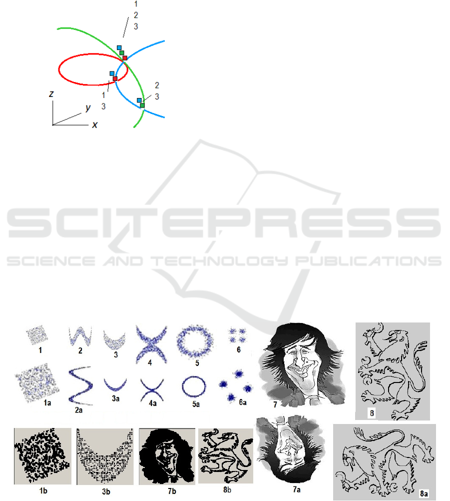
sizes for frequency. The identity is illustrated by the

example provided in Figure 1 that shows red (R),

green (G) and blue (B) curves intersecting at 3 points,

where columns emerge that contain names of these

curves. Obviously, the intersection size of G, B and

G, R patterns is

|| 2GB= and || 1GR= .

Figure 1: Red (1), green (2) and blue (3) intersecting curves

on (

)- coordinate plane.

At the same time, a histogram h of names

contained in the columns {2, 3} and {1, 2, 3], where

the green curve intersects the other lines, has the

samples

() 2hB =

and

() 1hR =

Hence,

|| ()GB hB= and || ()GR hR= ,

as it is stated in (3). Importantly, when columns

are available, all intersection sizes can be obtained by

scanning only three columns (in this example), even

though curves may be represented by thousands of

dots. Note that the above approach is similar to TF-

IDF method (Jones, 2004) developed for document

search or information retrieval, where inverse

document frequencies of the word across a set of

documents are calculated. This is a typical method

employed in search engines, where document name

frequencies in fully inverted files are calculated.

However, search engines will not work for pattern

recognition applications where textual inputs are

replaced with noisy numerical data. That is, not just

inverse document frequency of the word may change

depending on the currently available document

collection, but the word itself may completely

disappear because of even a small noise.

In case of numeric patterns, the objective is to

index each pattern by its features, for instance, the

edge pattern on the plain – by

(, )

- coordinates of

its dots. Then pattern identities would replace page

numbers of the back-of-book-index, where each set

, y

{}

contains identities of patterns that share the

coordinate pair

(, )

3.3 Introductory Example of

Indexing-Based Pattern

Recognition

Let consider a pattern recognition example where

elements of feature sets are 2D-features, which are

(, )

- coordinates of dark (below a certain grey

level) dots, that is, pixel coordinates are used as raw

features of image objects. Figure 2 shows an example,

where the shapes 1 - 8 are used for training and the

distorted shapes 1a - 8a are used for testing. Note that

for recognition of distorted objects 1a - 8a the

classification system should be invariant with respect

to scaling and orientation.

Figure 2: Pictures 1 – 8 (Wikipedia, 2022) were used for learning (single image per pattern class), pictures 1a – 8a (Wikipedia,

2022) are used for testing. Pictures 1b, 3b, 7b, 8b show outputs of a scale normalization algorithm when it takes in pictures

1, 3, 7, 8, respectively.

ICPRAM 2023 - 12th International Conference on Pattern Recognition Applications and Methods

224

Invariance with respect to scaling was achieved

by the normalization, whereby left-hand, right-hand,

upper and lower boundary coordinates

min max min max

,,,

xyy

were found and (

) -

coordinates of object’s dots were normalized to the

range

128D =

as follows

min max min

*( )/( )

Dxx x x=- -

min max min

*( )/( )yDyy y y=- -

Invariance with respect to orientation was

achieved by learning the objects 1 – 8 at a single view

angle and multiple recognition of objects 1a – 8a at

angles 0º through 360°, step 1º.

A notation for inverse patterns was introduced,

which is an indexed set

{}

n or

, y

{}

, where the set

element

is the name of a pattern class and the

indexes

are the feature values. The notation

, y

{}

helps to conveniently represent the algorithm

that calculates occurrence frequencies

, 1,...,

nN=

, of names in columns. Let , , 1,...,

yl L= be the

coordinates of dark dots, where L is the number of

dark dots in the current image (image 1 through 8).

Then name occurrence frequencies are best obtained

as samples of the histogram

Algorithm 1: Name histogram evaluation.

1,..., , , [ , ], { } :

ry s

lLrseenn

=∀∈−∀∈

ff=+

If classification of the current input image fails,

that is,

1,...,

max ( ) <

, then the new image class is

introduced, 1NN= + , and the columns are updated

using the Algorithm 2.

Algorithm 2: Updating of columns.

, ,

{} {} , 1,...,

ll ll

xy xy

nnNlL==

Here the initial conditions are

1N = ,

, ,

{} {1} , 1,...,

lll

xy xy

nlL==

But, the algorithm 1 cannot work properly as it

violates the exclusion rule from Section 1. That is, the

element

y of the current input pattern may be

accidentally compared within the loop

,[,]rs ee∀∈−

to more than one element of a previously stored

pattern (and visa versa). This is why columns and

class names must be inhibited once they have been

accessed, which is achieved by replacing histogram

algorithm 1 with the algorithm that inhibits patterns

by flagging dirty names

flag flag=→ = and

columns

, ,

0 = 1

xy xy

col col=→

. Then the

algorithm 1 can be re-written as Algorithm 3.

Algorithm 3: Histogram evaluation with inhibition.

1,..., , , 0, , [ , ],

l L n flag r s e e=∀ =∀∈−

{}

ry s

∀∈

if 0 and 0

xrys

col flag

1, 1, 1

nn n

xrys

f f col flag

=+ = =

Recognition accuracy (%) for distorted patterns 1a -

8a (Figure 2) at different neighborhood radiuses e is

provided in Table 1

Table 1: Recognition accuracy %.

e (pixels) 0 1 2 3 4

% 50 100 100 100 87.5

Figure 3: Some typical examples of commercial trademarks. Upper row images were used for training and bottom row images

were used for testing.

Random Quasi Intersections with Applications to Instant Machine Learning

225

Table 2: Recognition accuracy at testing of 1100 distorted commercial trademarks retrieved from (GoogleDrive, 2022).

e 0 1 2 3 4

% 98 100 100 100 99.2

3.4 Using Quasi-Intersections for

Commercial Trademark Image

Database

The same system was also trained on a database of

commercial trademarks, retrieved from

(GoogleDrive, 2022), which contains 1100 edge

images, each comprising 160 x 120 pixels (upper row

on the Figure 3 shows a few typical images out of

1100 images from this database). The training was

performed at

0e = . Next, 1100 distorted images

were used for testing (bottom row on the Figure 3

shows typical examples of distorted images and Table

2 shows the recognition accuracy.

The training time was shown to be about 3

seconds per 1000 images (pre-stored in RAM) on a

single core 1.6 GHz Intel Pentium CPU, which

amounts to 3 milliseconds per image. Although this

indexing-based non-iterative learning is impressively

fast, the burden of rotational invariance slows down

the recognition time by the factor of 360 amounting

to about 1 second per image).Pattern clustering may

emerge at learning if 0e > . But, the discussion of it is

beyond the scope of this paper

4 DISCUSSION

Whereas a classic intersection of two sets always

produces a single set, the quasi intersection definition

produces a multitude of possible intersections. But,

there is no way of knowing in advance which one of

them will emerge. Analogously, in quantum

mechanic, it is the quantum measurement that

localizes a particle, whose potential positions are

described by the wave function. And it is impossible

to predict, which slit the photon will go through until

a detector tells which way the particle had chosen.

Besides, the exclusion rule, whereby no two elements

of one set can simultaneously pair with one element

of the other set, reminds of Pauli Exclusion Principle

according to which no two identical fermions in any

quantum system can be in the same quantum state.

The discussed instant learning, like deep learning,

can work on raw features, which are image pixels,

meaning that no feature engineering is needed.

However, the scope of possible applications of

instant learning is not known as yet.

Implementation of quasi intersections implies

inhibition. Without inhibition the pattern scores

easily overflow expected levels, which resemble

brain circuitry organization, where excitatory neurons

are often accompanied by inhibitory neurons.

The objective of this paper is not a discussion of a

best way of implementing an image learning system,

but a proof-of-the-concept of quasi intersections

method. A better way of image recognition would be

a two or more level approach, where level 1 classifies

local features and level 2 classifies histograms of

classes of local features. Then subsets of histogram

samples will represent parts of input objects, which

resembles the activation pattern of the inferotemporal

brain region (Tsunoda et al., 2001). However, when

patterns are represented by feature vectors, rather

than feature sets, inhibition is not needed. The basics

of feature vectors’ indexing are provided in the

Appendix section.

REFERENCES

Brin S.and Page L.(1998). The Anatomy of a large-scale

hypotextual web search engine. In Computer Networks

and ISDN Systems Volume 30, Issues 1–7. Stanford

University, Stanford, CA, 94305, USA. Retrieved from

https://doi.org/10.1016/S0169-7552(98)00110-X

Sivic, J., Zisserman, A. (2009). Efficient visual search of

videos cast as text retrieval. ”. In IEEE Transactions on

Pattern Analysis and Machine Intelligence, Volume:

31, Issue: 4. doi: 10.1109/TPAMI.2008.111

Mikhailov A., Karavay M., Farkhadov M. ( 2017). Inverse

Sets in Big Data Processing. In Proceedings of the 11th

IEEE International Conference on Application of

Information and Communication Technologies

(AICT2017, Moscow). М.: IEEE, Vol. 1

https://www.researchgate.net/publication/321309177_

Inverse_Sets_in_Big_Data_Processing

Mikhailov, A., Karavay, M. (2021). Pattern Inversion as a

Pattern Recognition Method for Machine Learning. In

https://arxiv.org/abs/2108.10242.

Jaccard, P. (1901). Distribution de la flore alpine dans le

bassin des Dranses et dans quelques régions voisines.

In Bulletin de la Société Vaudoise des Sciences

Naturelles 37, 241 - 272.

Jones, K. (2004). A statistical interpretation of term

specificity and its application in retrieval . Journal of

ICPRAM 2023 - 12th International Conference on Pattern Recognition Applications and Methods

226

Documentation: MCB University: MCB University

Press, Vol. 60, no. 5. - P. 493 - 502. - ISSN 0022-0418.

Wikipedia. https://en.wikipedia.org/wiki/CorrelationGoogl

eDrive. https://drive.google.com/drive/u/0/folders/1t

ZmR7le1zbZb1Jpl_j4FYS5E-sjyVDVQ

Tsunoda K., Yamane Y., Nishizaki M., Tanifuji M. (2001).

Complex objects are represented in macaque

inferotemporal cortex by the combination of feature

columns. In Nat. Neurosci. 4 (8). pp.832-838.

doi:10.1038/90547. PMID 11477430

Mikhailov, A., Karavay, M. (2018). Inverse sets in Pattern

Recognition. Inverse Sets in Pattern Recognition.

Proceedings of IEEE East-West Design & Test

Symposium (EWDTS'2018). Kazan. IEEE EWDTS,

2018. С. 323-330.

APPENDIX

A.1 Patterns are Represented by

Feature Vectors

For feature vectors, there is no need to inhibit

accessed columns, even though the non-standard

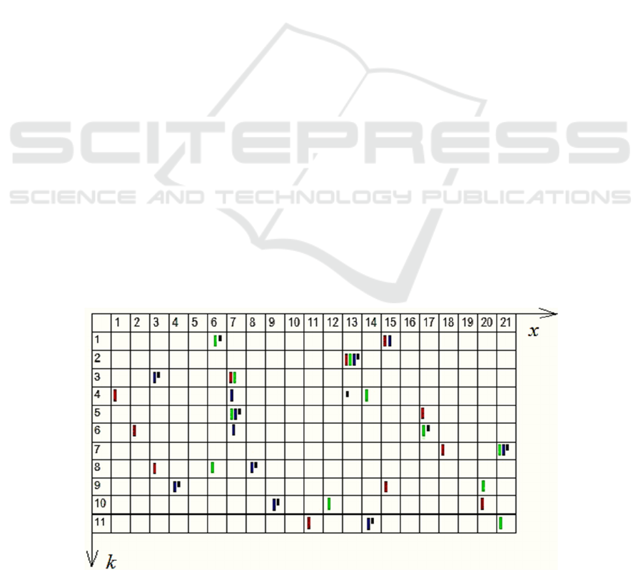
intersection definition (1) is used. Figure A.1

illustrates the above statement

In Figure A.1 example, x-coordinates of colored

marks represent component values of red, green and

blue 11-dimensional vectors, and k-coordinates

represent vectors’ component indexes. For instance,

the cell (15, 1) contains two vector names

, 15, 1

{} {1,3}

n =

. The cell (14, 4) contains the name

of the 2

vector and the cell (7, 3) contains names of

and 2

vectors.

The vector coordinate values are

(15,13,7,1,17,6,18, 3,15,20,11)

red

x =

)

(6,13,7,14,7,17,21,6, 20,12,21)

green

x =

)

(15,13,3,7,7,7,21,8,4,8,14)

blue

x =

)

(6,13,3,13,7,17,21,8,4,9,13)

black

x =

-dimensional space, the similarity between

vectors ,



can be evaluated as the intersection with

the size | | , 1,...,

en n

XX fn N== . For vectors,

this is always a single intersection because there

exists only one way of counting coordinate pairs. It is

an implication of the following two properties of

distinct vectors with integer components (

is the

range of component values, any cell and its content is

referred to as a column). Given

memorized vectors

(a) For each dimension

(for each horizontal

line), any two columns do not intersect

{} {} , ,

xk yk

nn xyD=∅ ∀ <



(b) For each dimension

, the sum of column

heights is equal to the number

of memorized vectors

|{ } |

−



It follows from (a), (b) that intersection sizes



 of the input vector

( ,..., ,..., )

xx x x=



with

memorized vectors , 1,...,

xn N=



, are equal to

frequencies

f of vector indexes in corresponding

columns

| | , 1,...,

xx fn N==





Computation of frequencies requires a definition

of inverse patterns that contain names of pattern

classes, feature sets or feature vectors.

Figure A.1: Feature vectors plain.

Random Quasi Intersections with Applications to Instant Machine Learning

227

A.2 Inverse Sets Definition

Given a collection of distinct sets

{ } , 1,...,

xn N==, inverse set

{}

contains

indexes of sets that share the element

{} { : },

nnxXxX

=∈ ∈



The sets/inverse sets transform

{ } , 1,..., { } ,

nxn

nNnxX

=↔ ∈



is a one-to-one correspondence.

Example. Given a collection of two sets

{,,}, {,, }abc bcd , inverse sets are

{1} , {1, 2} , {1, 2} , {2}

abcd

A.3 Inverse Patterns Definition

Let vectors in a K-dimensional space

, 1,..., , 1,...,

kKnN==

, differ in, at least, one

component

, : | |

nk mk

nm k x x e∀∃ − >

. Given N

such vectors, the inverse patterns are defined as

{ } { : | | }, , 1,...,

xk k

nnxxexDkK=−≤∈=

Here D is the range of vector components’ values.

Calculation of frequencies can be done by scanning

the content of

columns only, – even though

millions of base vectors may be given. This

replacement of similarities for frequencies minimizes

computational complexity of classification.

Frequencies are best obtained as samples of the

histogram of names found in inverse sets. In vector

case

, [ , ], { } : 1

xrk

kr ee nn f f

∀∀∈− ∀∈ = +

(A.1)

Here

( , 1,..., )

xk K==



is the input vector. The

input vector



is assigned to the most similar, that is,

most frequent class

1,...,

: max ( ), if

nin

nf f f t

(A.2)

where

is the recognition threshold. Properties

(a), (b) imply that, in vector case, maximal frequency

cannot exceed

A.4 Unsupervised Learning

Unsupervised learning starts with recognition. If

input vector



is successfully recognized using the

algorithm (A.1) and the expression (A.2), then

proceed to next input vector. If recognition fails, then

the number of classes is increased by 1 and the

collection of inverse patterns is updated by inserting

into the collection the name of the new class

1) 1NN=+

, ,

{ } { } , 1,...,

xk x

nnNkK==

Initial conditions are: 1N = ,

, ,

{ } {1} , 1,...,

xk xk

nkK==

Once the learning is done, the columns are no

longer updated. In case of supervised learning, the

teacher can introduce a look-up table

( ), 1,...,mclassnn N==

that relates created and

given classes.

A.5 Computational Complexity

Computational complexity of the frequency

algorithm (A.1) is proportional to the average height

of non-empty columns

, ,

(,)

|{ } |, {( , ):{ } }

xk xk

xk C

hnCxkn

∈

==≠∅



In turn, column height is inverse proportional to

variability radius e. The greater the radius e, the

bigger the generalization ability. As a result, less

classes N will be created, the average column height

will be reduced, which, in turn, decreases the

computational time. But, on the other hand, this

positive trend is limited by the declining

discriminating power of the system.

ICPRAM 2023 - 12th International Conference on Pattern Recognition Applications and Methods

228