Classiﬁcation and Embedding of Semantic Scene Graphs for Active

Cross-Domain Self-Localization

Yoshida Mitsuki, Yamamoto Ryogo, Wakayama Kazuki, Hiroki Tomoe and Tanaka Kanji

Graduate School of Engineering, University of Fukui, Fukui, Japan

Keywords:

Active Cross-Domain Self-Localization, Semantic Scene Graph, Scene Graph Classiﬁer, Scene Graph

Embedding.

Abstract:

In visual robot self-localization, semantic scene graph (S2G) has attracted recent research attention as a valu-

able scene model that is robust against both viewpoint and appearance changes. However, the use of S2G in the

context of active self-localization has not been sufﬁciently explored yet. In general, an active self-localization

system consists of two essential modules. One is the visual place recognition (VPR) model, which aims to clas-

sify an input scene to a speciﬁc place class. The other is the next-best-view (NBV) planner, which aims to map

the current state to the NBV action. We propose an efﬁcient trainable framework of active self-localization

in which a graph neural network (GNN) is effectively shared by these two modules. Speciﬁcally, ﬁrst, the

GNN is trained as a S2G classiﬁer for VPR in a self-supervised learning manner. Second, the trained GNN

is reused as a means of the dissimilarity-based embedding to map an S2G to the ﬁxed-length state vector. To

summarize, our approach uses the GNN in two ways: (1) passive single-view self-localization, (2) knowledge

transfer from passive to active self-localization. Experiments using the public NCLT dataset have shown that

the proposed framework outperforms other baseline self-localization methods.

1 INTRODUCTION

Cross-domain visual robot self-localization is the

problem of predicting the robot pose from on-board

camera image using an environment model (e.g.,

map), which was previously trained in different do-

mains (e.g., weathers, seasons, times of the day).

A large body of self-localization literature focuses

on designing or training the models that are ro-

bust to changes in appearance and viewpoint. Most

of them assume a single-view self-localization sce-

nario and do not consider viewpoint planning or ob-

server control issues. However, such a passive self-

localization problem is essentially ill-posed when cur-

rent live images are from a previously unseen do-

main. Existing solutions can be negatively inﬂuenced

by environmental and optical effects, such as occlu-

sions, dynamic objects, confusing features, illumi-

nation changes, and distortions. One promising ap-

proach to address this issue is to consider an active

self-localization scenario (Gottipati et al., 2019), in

which an active observer (i.e., robot) can adapt its

viewpoint trajectory, avoiding non-salient scenes that

provide no landmark view, or moving efﬁciently to-

wards places which are most informative, in the sense

of reducing the sensing and computation costs. This

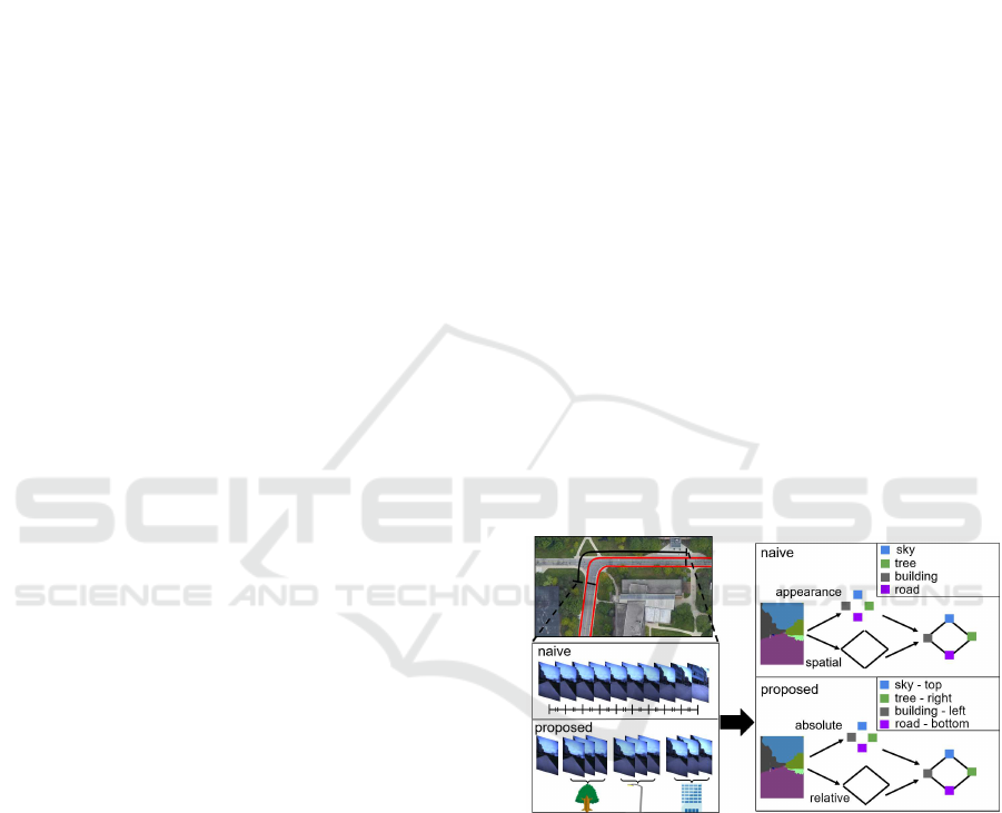
Figure 1: The nodes and edges in a semantic scene graph

represent the absolute attribute of an image region and the

relative attribute between a region pair, respectively.

is most closely related to the next-best-view (NBV)

problem studied in machine vision literature. How-

ever, in our cross-domain setting, a difﬁculty arises

from the fact that the NBV planner is trained and

tested in different domains. Existing NBV methods

that do not take into account domain shifts would be

confused and deteriorated by the domain-shifts, and

require signiﬁcant efforts for adapting them to a new

domain.

In this work, we present a novel framework for

active cross-domain self-localization based on the se-

562

Mitsuki, Y., Ryogo, Y., Kazuki, W., Tomoe, H. and Kanji, T.

Classiﬁcation and Embedding of Semantic Scene Graphs for Active Cross-Domain Self-Localization.

DOI: 10.5220/0011621200003417

In Proceedings of the 18th International Joint Conference on Computer Vision, Imaging and Computer Graphics Theory and Applications (VISIGRAPP 2023) - Volume 4: VISAPP, pages

562-569

ISBN: 978-989-758-634-7; ISSN: 2184-4321

 2023 by SCITEPRESS – Science and Technology Publications, Lda. Under CC license (CC BY-NC-ND 4.0)

mantic scene graph (S2G), as shown in Fig. 1. In

general, an active self-localization system consists of

two essential modules (Gottipati et al., 2019):

(1) Visual place recognition (VPR) model, to classify

an input scene to a speciﬁc place class;

(2) Next-best-view(NBV) planner, to map the current

state to the next-best-view action.

We are motivated by recent ﬁndings that S2G is a

valuable scene model that is robust to both view-

point and appearance changes (Gawel et al., 2018).

In our approach, a trainable S2G classiﬁer is effec-

tively shared by these two modules. Speciﬁcally, ﬁrst,

a graph neural network (GNN) is trained as the VPR

module in a self-supervised learning manner. Sec-

ond, the trained GNN is reused as an S2G embed-

ding model to transfer the state recognition ability of

the trained GNN to the NBV planner module. Ex-

periments using the public NCLT dataset (Carlevaris-

Bianco et al., 2016) have shown that the GNN clas-

siﬁer based on the semantic scene graph outperforms

other baseline self-localization methods. It was also

shown that the proposed dissimilarity-based graph

embedding generates good NBV action plans in the

NBV planning task.

2 RELATED WORK

2.1 Cross-Domain Self-Localization

Self-localization under changes in viewpoint and ap-

pearance is a challenging problem, and has been ex-

tensively studied (Lowry et al., 2016; Garg et al.,

2021; Zhang et al., 2021). Early works explored

local feature based self-localization approaches such

as bag-of-words (Cummins and Newman, 2011), in

which a query/map image is described by a collection

of local visual features. However, such a local feature

approach ignores contextual information (e.g., spatial

information) of the entire image, and is vulnerable to

changes in appearance caused by weather or seasonal

changes. To address this issue, some works employ

global features to improve robustness against appear-

ance changes. For example, GIST (Oliva and Tor-

ralba, 2001), a representative global feature, uses a

ﬁxed-length feature vector to precisely describe and

match the contextual information of the entire im-

age. However, since global features depend on the

information of the entire image, they are vulnerable

to viewpoint changes. Recently, attempts have been

made to improve the discriminative power of local

and global features using deep learning techniques

(Zhang et al., 2021). However, the vulnerability to

change is inherent in local and global visual features

and has not been overcome yet.

2.2 Semantic Scene Graphs

In recent years, semantic scene graphs (S2G) have

attracted attention from researchers as a robust self-

localization method under both appearance and view-

point changes (Gawel et al., 2018). A semantic scene

graph is an attributed graph whose nodes and edges

describe semantically attributed image regions and

relationship between them. Many studies have for-

mulated the S2G-based self-localization as a graph

matching problem (Kong et al., 2020). For exam-

ple, the X-View method in (Gawel et al., 2018) em-

ploys a graph matching algorithm based on random

walk to obtain improved robustness under appearance

and viewpoint changes. However, graph matching

techniques rely on structured pattern recognition al-

gorithms, and thus suffer from increasing computa-

tion cost. On the other hand, graph embeddings have

gained attention as a way to reduce the costly graph

matching problem to an efﬁcient machine learning

problem (Cai et al., 2018). However, its preprocess-

ing typically requires supervised learning of a graph

embedding model, which limits its applicability to

autonomous mobile robots. Recently, graph neural

network (GNN) has emerged as a means of machine

learning directly on general graph data without requir-

ing graph embedding. This has motivated us to use

the GNN classiﬁer as a method for visual place clas-

siﬁer.

2.3 Graph Embedding

The graph embedding formulation considered in our

study is most closely related to the dissimilarity-based

graph embedding scheme, one of representativegraph

embedding approaches in the ﬁeld of computer vi-

sion and pattern recognition (Borzeshi et al., 2013).

The dissimilarity-based embedding aims to describe

an input graph by its dissimilarity to a set of pre-

deﬁned prototype graphs. However, the choice of

dissimilarity measure is application dependent and

no general solution exists. Some methods employ

graph edit distance as a means of dissimilarity mea-

sure (Wang et al., 2021). However, such a structured

pattern recognition algorithm suffers from high com-

putational cost. Several recent works attempt to train

efﬁcient graph embedding models by deep learning.

However, they follow a supervised learning protocol

and require costly supervision, which is not available

in our autonomous robot applications. In contrast, our

approach reuses the pre-trained passive GNN classi-

Classiﬁcation and Embedding of Semantic Scene Graphs for Active Cross-Domain Self-Localization

563

ﬁer as the dissimilarity model. This approach is ap-

pealing in terms of training efﬁciency and real-time

performance. Speciﬁcally, the GNN classiﬁer can be

a novel computationally-efﬁcient dissimilarity mea-

sure, because it does not require costly structured-

pattern recognition nor supervised graph embedding

networks.

2.4 Next-Best-View Planners

Several researchers have studied the problem of next-

best-view planning for active robot self-localization.

In (Burgard et al., 1997), an active self-localization

task was addressed by extending the Markov local-

ization framework for action planning. In (Feder

et al., 1999), an appearance-based active observer

for a micro-aerial vehicle was presented. In (Chap-

lot et al., 2018), a deep neural network-based exten-

sion of active self-localization was addressed using

a learned policy model. In (Gottipati et al., 2019),

the policy model and the perceptual and likelihood

models were completely learned. In (Chaplot et al.,

2020), a neural network-based active SLAM frame-

work was investigated. However, these existing stud-

ies suppose in-domain scenarios, where the changes

in appearance and viewpoint between the training

and test domains was not signiﬁcant. The availabil-

ity of domain-invariant landmarks was often assumed

(e.g., (Tanaka, 2021)). In contrast, in our work, the

challenging cross-domain active self-localization sce-

nario is addressed by utilizing a deep graph neural

network in two ways: passive self-localization (i.e.,

visual place recognizer) and active self-localization

(i.e., next-best-view planner).

2.5 Relation to Existing Works

To our knowledge, this work is the ﬁrst to study se-

mantic scene graph (S2G) in the challenging sce-

nario of active cross-domain self-localization. Ex-

isting machine learning approaches require as input

ﬁxed-length feature vectors such as local and global

features. However, they had the limitation of being

vulnerable to changes in viewpoint and appearance.

Our approach employs a new scene model, the se-

mantic scene graph (S2G), which is robust to both

types of change. However, S2G is no longer a ﬁxed-

length feature vector, and thus cannot be dealt with by

most machine learning frameworks. The graph neu-

ral network (GNN) used in our research is a valuable

recently emerging machine learning framework that

can directly process graph data. Moreover, we ex-

plore to reuse the trained GNN as a means of embed-

ding an S2G to a ﬁxed vector, which is then used as

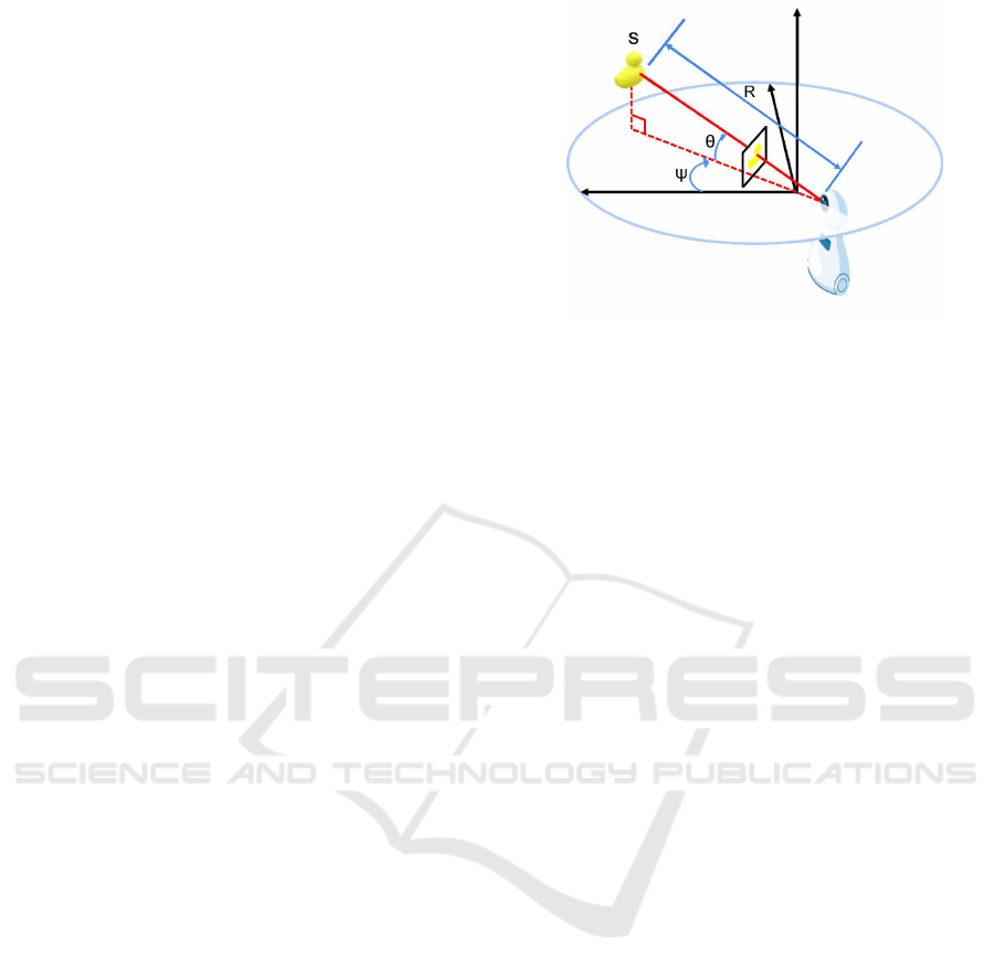
Figure 2: Bearing-range-semantic (BRS) measurement

model. The bearing, range, and semantics are observed in

an image, as the location, area, and semantic label, respec-

tively, of an object region. Then, the three-dimensional B-

R-S space is quantized to obtain a compact 189-dim 1-hot

vector (i.e., an 8-bit descriptor).

the discriminative state vector for training the view-

point planner. Consequently, in our approach, GNNs

are utilized not only as passive S2G classiﬁers, but

also as a means of knowledge transfer from passive to

active self-localization.

3 APPROACH

The proposed framework consists of two main mod-

ules: (ofﬂine) training module and (online) test mod-

ule. In addition, a scene graph descriptor sub-module

is employed by the both modules. These modules are

detailed in the following subsections.

3.1 Semantic Scene Graph

We employ a simple bottom-up procedure for scene

parsing, to generate a semantic scene graph from a

given query/map image. First, semantic labels are

assigned to pixels using DeepLab v3+ (Chen et al.,

2018), which was pretrained on Cityscapes dataset.

Then, regions smaller than 100 pixels are regarded as

not characterizing the input scene, and removed. Sub-

sequently, connected regions with the same semantic

labels are identiﬁed using a ﬂood-ﬁll algorithm (He

et al., 2019), and each region is assigned a unique re-

gion ID. Next, each region is connected to each of

its adjacent regions by a graph edge. As a result, a

semantic scene graph with the nodes and edges de-

scribed above is obtained.

We observe that not only semantic information but

also spatial information is important in the robotic

applications. This spatial information is particularly

important in the SLAM ﬁeld, and existing SLAM

frameworks are classiﬁed into several categories ac-

VISAPP 2023 - 18th International Conference on Computer Vision Theory and Applications

564

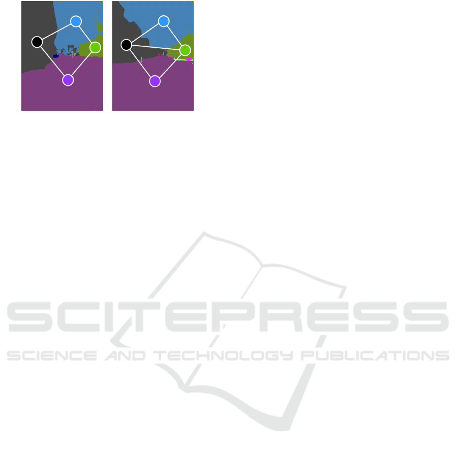
Figure 3: Using edges enables to distinguish between two

similar but different scene layouts, as in this example.

cording to the type of spatial information, such as

range-bearing SLAM (Ramezani et al., 2020), range-

only SLAM (Song et al., 2019), and bearing-only

SLAM (Bj et al., 2017). Our problem formulation

falls into an alternative category of bearing-range-

semantic (BRS) -based self-localization (Fig. 2).

Speciﬁcally, in our approach, a semantic scene

graph is computed in the following procedure.

First, the semantic labels output by a seman-

tic segmentation network in (Ronneberger et al.,

2015) were re-categorized into seven different se-

mantic category IDs: “sky,” “tree,” “building,”

“pole,” “road,” “trafﬁc sign,” and “the others”

which respectively correspond to the labels {“sky”},

{“vegetation”}, {“building”}, {“pole”}, {“road,”

“sidewalk”}, {“trafﬁc-light,” “trafﬁc-sign”}, and

{“person,” “rider,” “car,” “truck,” “bus,” “train,” “mo-

torcycle,” “bicycle,” “wall,” “fence,” “terrain”} in the

original label space. The location of the region center

was quantized into nine “bearing” category IDs by a

3×3 regular grid imposed on the image frame. Area

of the region was quantized into three “range” cate-

gory IDs: “short distance (larger than 150 K pixels),”

“medium distance (50 K-150 K pixels),” and “long

distance (smaller than 50 K)” for 616×808 image. Fi-

nally, these semantic, bearing and range category IDs

are combined to obtain a (7×3×9=) 189-dim 1-hot

vector as the node descriptor.

We observe that the nodes and edges represent two

different aspect of the spatial information, which can

act as error detection codes (C´orcoles et al., 2015) that

complement each other. Speciﬁcally, an edge is suit-

able for describing the relative feature (e.g., position-

relationship), while a node is suitable for describing

the absolute feature (e.g., position). Figure 3 illus-

trates an example showing how the use of edge infor-

mation helps to discriminate a near-duplicate scene

pair, which the node descriptor alone could not dis-

criminate.

We also adopted a region merging technique, in-

spired by a recent work in (Matejek et al., 2019).

Speciﬁcally, we remove regions smaller than 1,000

pixels (for 616×808 image). We noted this sim-

ple technique to be quite effective in improving self-

localization performance.

3.2 Visual Place Recognition

Self-localization from semantic scene graph is di-

rectly addressed by graph convolutional neural net-

work (GCN) (Wang et al., 2019) -based visual place

classiﬁer. GCN is one of most popular approaches to

graph neural networks. Speciﬁcally, we aim to train a

GCN as a visual place classiﬁer, which takes a single-

view image and predicts the place class.

For the deﬁnition of place classes, we follow the

grid-based partitioning in (Kim et al., 2019). In

the experimental environment, this yields 10×10 grid

cells and 100 place classes in total.

In this study, a GCN is trained by using the se-

mantic scene graphs as the training data. The graph

convolution operation takes a node v

in the graph and

processes it in the following manner. First, it receives

messages from nodes connected by the edge. The

collected messages are then summed via the SUM

function. The result is passed through a single-layer

fully connected neural network followed by a non-

linear transformation for conversion into a new fea-

ture vector. In this study, we used the rectiﬁed lin-

ear unit (ReLU) operation as the nonlinear transfor-

mation. The process was applied to all the nodes in

the graph in each iteration, yielding a new graph that

had the same shape as the original graph but updated

node features. The iterative process was repeated L

times, where L represents the ID of the last GCN

layer. After the graph node information obtained in

this manner were averaged, the probability value vec-

tor of the prediction for the graph was obtained by

applying the fully connected layer and the softmax

function. For implementation, we used the deep graph

library (Wang et al., 2019) on the Pytorch backend.

In the multi-view self-localization scenario, the

latest viewimage/odometry measurement at each time

is incrementally fused into the belief state. For the

information fusion, the standard Bayes ﬁlter-based

information fusion as in (Dellaert et al., 1999) is

adopted. The motion and perception models of the

Bayes ﬁlter are adopted to our speciﬁc application do-

main. Speciﬁcally, a motion corresponds to a forward

move along the viewpoint trajectory, and a percep-

tion corresponds to a class-speciﬁc probability den-

sity vector (PDV) output by the GCN. In implementa-

tion, a slightly simpliﬁed motion and perception mod-

els are used. First, the marginalization step associated

with the robot motion model was skipped by utiliz-

ing a noise-free motion model. Then, the Bayes rule

Classiﬁcation and Embedding of Semantic Scene Graphs for Active Cross-Domain Self-Localization

565

step associated with the robot perception model was

replaced with a reciprocal rank fusion operation in

(Cormack et al., 2009).

The spatial resolution of the Bayes ﬁlter state

space (e.g., 1 m) is required to be the same or higher

than that of the odometer sensor, which is much

higher than that of the state space of visual place clas-

siﬁer. Conversionbetween two state vectors with such

different spatial resolutions is simply implemented as

a marginalization operation.

3.3 Next-best-View Planning

The next-best-view planning is formulated as a

reinforcement-learning (RL) problem, in which a

learning agent interacts with a stochastic environ-

ment. The interaction is modeled as a discrete-time

discounted Markov decision process (MDP). A dis-

counted MDP is a quintuple (S, A, P, R, γ), where S

and A are the set of states and actions, respectively.

P denotes the state transition distribution, R denotes

the reward function, and γ ∈ (0, 1) denotes a discount

factor (γ = 0.9). The learning rate was set to α =0.1.

We denoted P(·|s, a) and r(s, a) as the probability dis-

tribution over the next state and the immediate reward

of performing an action a for a state s, respectively.

Speciﬁcally, the state s is deﬁned as the class-speciﬁc

reciprocal rank vector, output by the GCN classiﬁer.

The action a is deﬁned as a forward movement along

the route.

In the experiments, we use a speciﬁc implementa-

tion as shown below. The action set is a size 10 set of

candidates of forward movement along the predeﬁned

trajectories A ={1, 2, · ·· , 10} (m). Each training/test

episode is a length n = 4 perception-plan-action se-

quence. The RL is trained by the recently developed

efﬁcient RL scheme of nearest neighbor Q-learning

(NNQL) (Shah and Xie, 2018) with neighborhood

factor k = 4. The immediate reward is provided at

the ﬁnal viewpoint of each training episode, as the re-

ciprocal rank value of the ground truth place-class.

4 EXPERIMENTS

The proposed method was evaluated in an active

cross-domain self-localization scenario. The goal of

the evaluation was to validate whether the GCN-based

classiﬁer and embedding of semantic scene graph

could boost the performance in both the passive and

active self-localization modules.

Figure 4: Experimental environments. The trajectories

of the four datasets, “2012/1/22,” “2012/3/31,” “2012/8/4,”

and “2012/11/17,” used in our experiments are visualized in

green, purple, blue, and light-blue curves, respectively.

4.1 Dataset

The public NCLT long-term autonomy dataset

(Carlevaris-Bianco et al., 2016) was used in the ex-

periments (Fig. 4). The dataset was collected through

multi-session navigation under various weather, sea-

sons and times of day over multiple years using a

Segway vehicle at the University of Michigan North

Campus. While the vehicle travels seamlessly in-

doors and outdoors, the vehicle encountered various

geometric changes (e.g., object placement changes,

pedestrians, car parking/stopping) and photometric

changes (e.g., lighting conditions, shadows, and oc-

clusions).

In particular, we supposed a challenging cross-

season self-localization scenario, in which the self-

localization system is trained and tested in differ-

ent seasons (i.e., domains). Speciﬁcally, four sea-

sons’ datasets “2012/1/22 (WI),” “2012/3/31 (SP),”

“2012/8/4 (SU),” and “2012/11/17 (AU)” were used

to create four different training-test seasons pairs:

(WI, SP), (SP, SU), (SU, AU), and (AU, WI). Addi-

tionally, an extra season “2012/5/11 (EX)” was used

to train the visual place classiﬁer. That is, the clas-

siﬁer was trained only once in the season EX, prior

to the self-localization tasks, and then the learned

classiﬁer parameters were commonly used for all the

training-test season pairs. The number of training and

test episodes were 10,000 and 1,000, respectively.

4.2 Comparing Methods

Three different self-localization methods, GCN, naive

Bayes nearest neighbor (NBNN), and k-nearest

neighbor (kNN) were evaluated. The GCN is the

proposed method that uses GCN in two ways, VPR

and NBV from a semantic scene graph (S2G), as de-

scribed in Section 3. Other comparing methods are

non-S2G-based methods, which ignore graph edges

and represent an input image as a collection of image

VISAPP 2023 - 18th International Conference on Computer Vision Theory and Applications

566

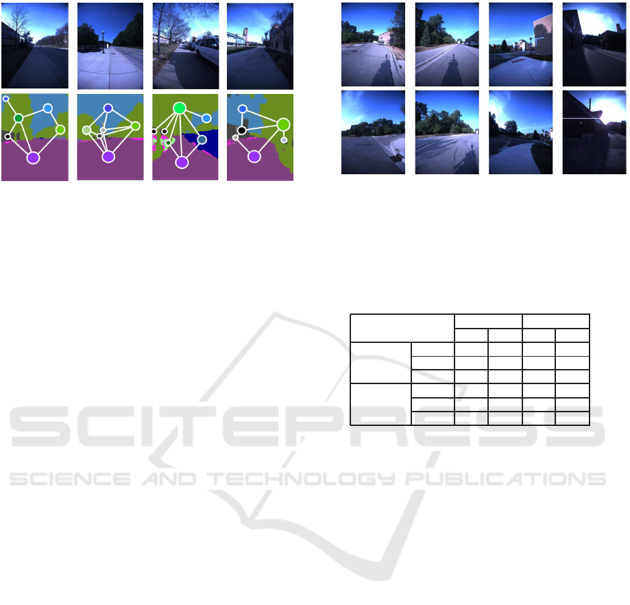
(a) (b) (c) (d)

Figure 5: Examples of semantic scene graph. Top: The in-

put scene. Bottom: The corresponding scene graphs over-

laid on the semantic label image.

regions. For fair comparison, the same node regions

used in the proposed method were used as the image

regions in the comparing methods. NBNN and kNN

methods are based on measuring dissimilarities in the

node feature set between a query-map pair of inter-

est. NBNN (Tommasi and Caputo, 2013) is one of

the best known methods to measure dissimilarities be-

tween such a feature set pair. In that, the L2 distance

from the nearest-neighbor map feature to each query

feature is computed, and then it is averaged over all

the query features, which yields the NBNN dissimi-

larity value. kNN is a traditional non-parametric clas-

siﬁcation method based on the nearest-neighbor train-

ing sample in the feature space, in which the class la-

bels most often assigned to the training samples of the

kNN (i.e., minimum L2 norm) are returned as classi-

ﬁcation results. In that, an image is described by a

189-dim histogram vector by aggregating all the node

features that belong to the image.

4.3 Performance Index

Self-localization performance was evaluated in terms

of top-1 accuracy. The evaluation procedure was as

follows. First, self-localization performance at all

viewpoints of the query episode, and not just the ﬁ-

nal viewpoint, were computed. Then, top-1 accuracy

at each viewpoint was computed from the latest Bayes

ﬁlter output based on whether the class with highest

belief value matches the ground-truth.

4.4 Results

Figure 5 shows semantic scene graphs used in the ex-

periments. Notably, the domain-invariant scene parts

(e.g., buildings and roads) of the input scenes tended

to be selected as the dominant parts.

Figure 6 shows examples of views before and after

(a) (b) (c) (d)

Figure 6: Next-best-view planning results. In each ﬁgure,

the bottom and top panels show the view image before and

after the planned next-best-view actions, respectively.

Table 1: Performance results.

“RM”: region merging, “S”: semantic, “BRS”: bearing-range-semantic,

“VPR”: visual place recognition (w/ random action planning),

“VPR+NBV”: VPR w/ next-best-view planning

w/ RM w/o RM

S BRS S BRS

GCN 11.7 18.9 12.0 19.1

VPR kNN 5.8 15.6 6.3 12.9

NBNN 1.3 3.4 1.4 3.5

GCN 19.9 31.4 19.5 32.3

VPR+NBV kNN 10.9 28.4 11.2 24.8

NBNN 2.2 4.7 2.7 4.6

planned next-best-view actions. Intuitively convinc-

ing behavior of the robot was observed. Before the

move, the scene was a non-salient one consisting only

of the sky, the road, and the trees (Fig. 6 a,b,c), or the

ﬁeld of view was very narrow due to occlusions (Fig.

6d). After the move, landmark objects came into view

(Fig. 6 a,c) or additional landmarks appeared (Fig. 6

b,d). Such behaviors are intuitively appropriate and

effective for seeking and tracking landmarks when a

human becomes lost and looks for familiar landmark

objects. Our approach enables the robot to learn such

an appropriate state-to-action mapping from available

visual experience.

Series of experiments were conducted to observe

the effects of individual components, including the

graph edges and the region merging. Table 1 lists

the results of the proposed next-best-view planner

(“VPR+NBV”) and a baseline planner with random

action planning (“VPR”). Moreover, we compared

the proposed BRS-based region descriptor (“BRS”)

with the baseline semantic label-based region descrip-

tor (“S”). Notably, the proposed method yielded a su-

perior performance compared to the other methods.

The technique of region merging contributed to re-

duce the number of nodes while retaining the self-

localization performance. The number of nodes was

reduced from 19.8 to 7.2 per semantic scene graph on

Classiﬁcation and Embedding of Semantic Scene Graphs for Active Cross-Domain Self-Localization

567

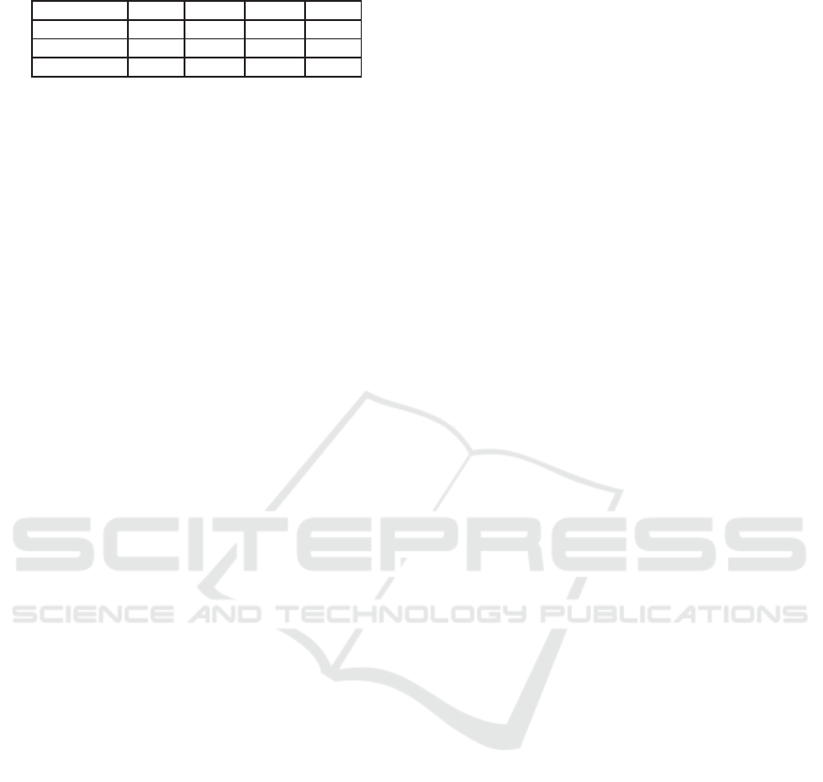
Table 2: Ablation studies.

Training-Test SP-SU SU-AU AU-WI WI-SP

BRS regions 23.8 14.8 15.3 21.7

BRS image 21.4 13.9 13.7 20.1

B-R-S regions 20.1 12.2 13.7 19.2

average, which results in the reduction of computa-

tion time for self-localization from 0.82 ms to 0.16

ms. Particularly, the use of edge feature and the next-

best-view planner often signiﬁcantly boosted the self-

localization performance.

Table 2 lists the results of additional ablation

studies. Here, we veriﬁed the importance of graph

topology and region descriptors. In the table, “BRS

regions” and “B-R-S regions” use semantic scene

graphs based on segmentation, but have different de-

scriptors for region nodes. “BRS regions” is the

proposed method that represents region nodes by a

1-hot vector in the discretized joint space of bear-

ing range semantics. “B-R-S regions” is an alterna-

tive method that ﬁrst computes 1-hot vectors inde-

pendently in each of the three discretized spaces of

bearing, range, and semantics, and then concatenate

the three 1-hot vectors to obtain a 3-hot state vector

(“B-R-S regions”). “BRS image” differs from “BRS

regions” only in terms of graph topology, and uses a

single-node semantic scene graph with the entire im-

age as a graph node. From this table, we can see that

the proposed method, which describes the semantic

scene graph consisting of region nodes using 1-hot re-

gion descriptors of the BRS joint space, outperforms

the other methods.

We observe that the descriptor compactness is

quite important in the training phase because the re-

inforcement learning procedure iterates the classiﬁ-

cation process for hundreds of thousands of times

through the training episodes. In our approach, suf-

ﬁciently compact scene descriptor was acquired by

the proposed approach, as shown bellow. The num-

ber of nodes per semantic scene graph was 7.2 on av-

erage. The node descriptor consumed 8-bit per node.

The space cost for nodes and edges were 57.8-bit and

12.5-bit per semantic scene graph, respectively, on

average. This a low space cost, even compared to

the most compact existing descriptors such as bag-

of-words. Notably, the current descriptors were not

compressed, i.e., they may be further compressed.

5 CONCLUDING REMARKS

In this paper, a new trainable framework for ac-

tive cross-domain self-localization by using the se-

mantic scene graph model is presented. In the pro-

posed framework, graph neural networks (GNNs) are

used in two ways. First, the GNN is trained as a

visual place classiﬁer for passive single-view self-

localization in the fashion of self-supervised learning.

Second, the trained GNN is reused as a means of em-

bedding S2G into a ﬁxed-length state vector, which is

then fed to the reinforcement learning module to train

the next-best-view planner. Experiments showed that

the proposed method is effective in both passive self-

localization and knowledge transfer from passive to

active self-localization. The proposed framework was

found to be robust to changes in both viewpoint and

appearance. In the future, we plan to clarify these ro-

bustness and limitations through further research us-

ing real robots as well as simulated environments.

REFERENCES

Bj, E., Johansen, T. A., et al. (2017). Redesign and analysis

of globally asymptotically stable bearing only slam.

In 2017 20th International Conference on Information

Fusion (Fusion), pages 1–8. IEEE.

Borzeshi, E. Z., Piccardi, M., Riesen, K., and Bunke,

H. (2013). Discriminative prototype selection meth-

ods for graph embedding. Pattern Recognition,

46(6):1648–1657.

Burgard, W., Fox, D., and Thrun, S. (1997). Active mobile

robot localization. In Proceedings of the Fifteenth In-

ternational Joint Conference on Artiﬁcial Intelligence,

IJCAI, pages 1346–1352. Morgan Kaufmann.

Cai, H., Zheng, V. W., and Chang, K. C.-C. (2018). A com-

prehensive survey of graph embedding: Problems,

techniques, and applications. IEEE Transactions on

Knowledge and Data Engineering, 30(9):1616–1637.

Carlevaris-Bianco, N., Ushani, A. K., and Eustice, R. M.

(2016). University of michigan north campus long-

term vision and lidar dataset. The International Jour-

nal of Robotics Research, 35(9):1023–1035.

Chaplot, D. S., Gandhi, D., Gupta, S., Gupta, A., and

Salakhutdinov, R. (2020). Learning to explore using

active neural SLAM. In 8th International Conference

on Learning Representations.

Chaplot, D. S., Parisotto, E., and Salakhutdinov, R. (2018).

Active neural localization. In 6th International Con-

ference on Learning Representations.

Chen, L.-C., Zhu, Y., Papandreou, G., Schroff, F., and

Adam, H. (2018). Encoder-decoder with atrous sepa-

rable convolution for semantic image segmentation. In

Proceedings of the European conference on computer

vision (ECCV), pages 801–818.

C´orcoles, A. D., Magesan, E., Srinivasan, S. J., Cross,

A. W., Steffen, M., Gambetta, J. M., and Chow, J. M.

(2015). Demonstration of a quantum error detection

code using a square lattice of four superconducting

qubits. Nature communications, 6(1):1–10.

Cormack, G. V., Clarke, C. L., and Buettcher, S. (2009).

Reciprocal rank fusion outperforms condorcet and in-

dividual rank learning methods. In Proceedings of

VISAPP 2023 - 18th International Conference on Computer Vision Theory and Applications

568

the 32nd international ACM SIGIR conference on

Research and development in information retrieval,

pages 758–759.

Cummins, M. and Newman, P. M. (2011). Appearance-

only SLAM at large scale with FAB-MAP 2.0. Int. J.

Robotics Res., 30(9):1100–1123.

Dellaert, F., Fox, D., Burgard, W., and Thrun, S. (1999).

Monte carlo localization for mobile robots. In 1999

International Conference on Robotics and Automation

(ICRA), volume 2, pages 1322–1328.

Feder, H. J. S., Leonard, J. J., and Smith, C. M.

(1999). Adaptive mobile robot navigation and map-

ping. The International Journal of Robotics Research,

18(7):650–668.

Garg, S., Fischer, T., and Milford, M. (2021). Where is

your place, visual place recognition? In Zhou, Z.-

H., editor, Proceedings of the Thirtieth International

Joint Conference on Artiﬁcial Intelligence, IJCAI-21,

pages 4416–4425. International Joint Conferences on

Artiﬁcial Intelligence Organization.

Gawel, A., Del Don, C., Siegwart, R., Nieto, J., and Cadena,

C. (2018). X-view: Graph-based semantic multi-view

localization. IEEE Robotics and Automation Letters,

3(3):1687–1694.

Gottipati, S. K., Seo, K., Bhatt, D., Mai, V., Murthy, K.,

and Paull, L. (2019). Deep active localization. IEEE

Robotics and Automation Letters, 4(4):4394–4401.

He, Y., Hu, T., and Zeng, D. (2019). Scan-ﬂood ﬁll(scaff):

An efﬁcient automatic precise region ﬁlling algorithm

for complicated regions. In IEEE Conference on

Computer Vision and Pattern Recognition Workshops,

pages 761–769. Computer Vision Foundation / IEEE.

Kim, G., Park, B., and Kim, A. (2019). 1-day learning, 1-

year localization: Long-term lidar localization using

scan context image. IEEE Robotics and Automation

Letters, 4(2):1948–1955.

Kong, X., Yang, X., Zhai, G., Zhao, X., Zeng, X., Wang,

M., Liu, Y., Li, W., and Wen, F. (2020). Semantic

graph based place recognition for 3d point clouds. In

2020 IEEE/RSJ International Conference on Intelli-

gent Robots and Systems (IROS), pages 8216–8223.

IEEE.

Lowry, S. M., S¨underhauf, N., Newman, P., Leonard, J. J.,

Cox, D. D., Corke, P. I., and Milford, M. J. (2016).

Visual place recognition: A survey. IEEE Trans.

Robotics, 32(1):1–19.

Matejek, B., Haehn, D., Zhu, H., Wei, D., Parag, T., and

Pﬁster, H. (2019). Biologically-constrained graphs for

global connectomics reconstruction. In Proceedings

of the IEEE/CVF Conference on Computer Vision and

Pattern Recognition, pages 2089–2098.

Oliva, A. and Torralba, A. (2001). Modeling the shape

of the scene: A holistic representation of the spatial

envelope. International journal of computer vision,

42(3):145–175.

Ramezani, M., Tinchev, G., Iuganov, E., and Fallon, M.

(2020). Online lidar-slam for legged robots with ro-

bust registration and deep-learned loop closure. In

2020 IEEE International Conference on Robotics and

Automation (ICRA), pages 4158–4164. IEEE.

Ronneberger, O., Fischer, P., and Brox, T. (2015). U-

net: Convolutional networks for biomedical image

segmentation. In Medical Image Computing and

Computer-Assisted Intervention, volume 9351 of Lec-

ture Notes in Computer Science, pages 234–241.

Springer.

Shah, D. and Xie, Q. (2018). Q-learning with nearest neigh-

bors. In Advances in Neural Information Processing

Systems 31: Annual Conference on Neural Informa-

tion Processing Systems, pages 3115–3125.

Song, Y., Guan, M., Tay, W. P., Law, C. L., and Wen, C.

(2019). Uwb/lidar fusion for cooperative range-only

slam. In 2019 international conference on robotics

and automation (ICRA), pages 6568–6574. IEEE.

Tanaka, K. (2021). Active cross-domain self-localization

using pole-like landmarks. In 2021 IEEE Interna-

tional Conference on Mechatronics and Automation

(ICMA), pages 1188–1194.

Tommasi, T. and Caputo, B. (2013). Frustratingly easy nbnn

domain adaptation. In Proceedings of the IEEE Inter-

national Conference on Computer Vision, pages 897–

904.

Wang, M., Yu, L., Zheng, D., Gan, Q., Gai, Y., Ye, Z., Li,

M., Zhou, J., Huang, Q., Ma, C., Huang, Z., Guo, Q.,

Zhang, H., Lin, H., Zhao, J., Li, J., Smola, A. J., and

Zhang, Z. (2019). Deep graph library: Towards ef-

ﬁcient and scalable deep learning on graphs. ICLR

Workshop on Representation Learning on Graphs and

Manifolds.

Wang, R., Zhang, T., Yu, T., Yan, J., and Yang, X. (2021).

Combinatorial learning of graph edit distance via dy-

namic embedding. In Proceedings of the IEEE/CVF

Conference on Computer Vision and Pattern Recogni-

tion, pages 5241–5250.

Zhang, X., Wang, L., and Su, Y. (2021). Visual place recog-

nition: A survey from deep learning perspective. Pat-

tern Recognition, 113:107760.

Classiﬁcation and Embedding of Semantic Scene Graphs for Active Cross-Domain Self-Localization

569