A Simulation Tool for Exploring Ammunition Stockpile Dynamics

Jean-Denis Caron, Robert Mark Bryce and Chad Young

Defence Research and Development Canada (DRDC) – Centre for Operational Research and Analysis (CORA),

Keywords:

Ammunition, Discrete-Event Simulation, Military, Stockpile.

Abstract:

The Canadian Armed Forces (CAF) uses ammunition of various types for both training and operations. We in-

troduce a Discrete-Event Simulation (DES) model, named Future Event Ammunition Stockpile Tool (FEAST),

to explore issues regarding anticipated stockpile drawdown and resupply. Schedules for military training and

operations and associated ammunition demands are stochastically deﬁned as inputs to FEAST, as are budgets,

various reorder policies and other inventory management parameters. Outputs of FEAST enable statistical

characterization of various performance attributes, including anticipated fulﬁllment of demands and costs over

time. FEAST is designed to be ﬂexibly used by practitioners to answer “what if” type questions. This paper

provides an overview of FEAST and illustrates a simpliﬁed scenario where a single nature of ammunition is

required to simultaneously fulﬁll demands from several training types and military missions, for which several

resupply options are to be explored.

1 INTRODUCTION

1.1 Background

Live ammunition is foundational for projecting mil-

itary power and it is used by modern militaries in

the context of Force Generation (FG) (i.e., military

training at individual and collective levels) and Force

Employment (FE) (i.e., during employment of mili-

tary forces in operational theatres). Adequate stocks

of ammunition are required to meet future demands,

which generally are only partially known. Procure-

ment of ammunition supply to meet this demand is

complicated by many factors: long procurement lead

times (of months to years), high costs, technological

obsolescence, ﬁnite shelf life, limited industry pro-

duction capacity, and stringent storage requirements

which limits storage capacity. Mindful of these un-

certainties and complicating factors, stockpiles of am-

munition help to ensure adequate fulﬁllment of am-

munition requirements over time by creating a buffer

between the receipt of incoming supplies and the al-

location of these supplies to meet demands. In so

doing, the costs of maintaining stockpile levels, as

well as management and storage constraints, must

also be balanced with risks associated with falling

below stock level thresholds. Taken together within

a dynamic system with multiple stakeholders that

changes over time all of these issues make it chal-

lenging for practitioners to understand and commu-

nicate the marginal impacts of changing conditions,

support decision making, and set new performance

targets, management policies, or forward plans.

To help improve the management of ammuni-

tion, the Centre for Operational Research and Anal-

ysis (CORA), part of Defence Research and Develop-

ment Canada (DRDC), undertook to aid the Depart-

ment of National Defence (DND) and the Canadian

Armed Forces (CAF) with determining the need for

various ammunition types (i.e., natures) and address

stockpiling questions pertinent to particular ﬂeets and

across the force structure where approximately 400

various natures are used. To support this we designed

a stockpile simulation tool, which is named Future

Event Ammunition Stockpile Tool (FEAST).

FEAST is a Discrete-Event Simulation (DES) tool

that aims to be ﬂexible and general, with parameters

being described by probability distributions where ap-

propriate, allowing both demand and supply to be

stochastic processes. Prices, including penalties for

stockout, are incorporated and parameters can change

over time. For example, annual budgets can be set,

and demands and procurement can be deﬁned in time

windows. FEAST intentionally has limited analysis

features built-in to keep focused scope, and outputs

sufﬁciently rich data for subsequent post-processing

and analysis.

Caron, J., Bryce, R. and Young, C.

A Simulation Tool for Exploring Ammunition Stockpile Dynamics.

DOI: 10.5220/0011620800003396

In Proceedings of the 12th International Conference on Operations Research and Enterprise Systems (ICORES 2023), pages 38-49

ISBN: 978-989-758-627-9; ISSN: 2184-4372

 2023 by His Majesty the King in Right of Canada as represented by the Minister of National Defence and SCITEPRESS – Science and Technology Publications, Lda. Under

CC license (CC BY-NC-ND 4.0)

1.2 Outline

This paper contains four more sections and one ap-

pendix. Section 2 provides an outline of the stock-

piling problem, related work, and the implementation

of FEAST, which touches upon the DES modelling

paradigm, the main assumptions and modeling fea-

tures, and the inputs and outputs. Section 3 intro-

duces a notional case study pertinent to a segment of

the CAF which has been simpliﬁed, altered and re-

stricted to a single ammunition nature for purposes of

presentation herein. For example, demand has been

modiﬁed from a subset of FG and FE requirements.

Section 4 includes a discussion on practical consid-

erations for usage of the tool, limitations and some

aspects under development. Concluding comments

are made in Section 5. Finally two veriﬁcation cases

are presented in the Appendix for which the simu-

lated output can be compared to the expected annual

steady-state demand for ammunition.

2 THE FUTURE EVENT

AMMUNITION STOCKPILE

TOOL

FEAST is driven in a “black box” manner by specify-

ing inputs. Here we sketch some approaches to stock-

piling and introduce the key features and elements of

FEAST.

2.1 Approaches to Stockpiling

Approximate Dynamic Programming (ADP) is a

widely used approach for operational research ques-

tions involving sequential decisions under uncer-

tainty. ADP has been applied to help optimize in-

ventory management policies (Powell, 2009) and to

address a variety of other challenges facing the mil-

itary (Rempel and Cai, 2021). At its core, ADP is

a discrete-time approach where the state of the sys-

tem transitions under a decision based on observed

information and there is a cost/reward associated with

how decisions play out. With these elements ADP

attempts to ﬁnd functions, or policies, that optimally

map the k-th state to the k-th decision. In terms of

stockpiling, the state encodes the stockpile, the infor-

mation is the (generally stochastic) demand over the

time period, the decision is the amount of ammuni-

tion to purchase in that time step, and the costs are

ordering, storage, and stockout penalty (real or vir-

tual) costs. While ADP is a powerful and general

framework, demand is required as an input, a suit-

able time step size selected, and constraints on good

policies to be searched for imposed. Here we will

be focusing on more primary concerns, considering

a rolling-horizon approach (Powell, 2009) to gener-

ate demand and ask “what if” questions, leaving opti-

mization concerns and approaches that further exploit

these elements for future work.

For ammunition stockpiling, more pedestrian ap-

proaches are often taken due to the numerous con-

straints, complicating factors, and unknowns in-

volved. For example, one complicating factor is

that a national stockpile is not a single reserve,

but is partitioned into several sub-stockpiles, includ-

ing those reserved for ongoing operations, train-

ing, war contingency, experiments and disposal (see

page 77 of (Brown, 2008)). Additionally, stock-

piles are physically partitioned and located in differ-

ent places geographically, e.g., at continental hold-

ings, off-continent support hubs, and deployed bases

(Bacot, 2009). Another complicating factor is man-

ufacturer stockpiles awaiting sale and partner stock-

piles are “potential” stockpiles as they are extant but

there may be limited visibility into, and uncertainty

ability to draw from, these sources and it is difﬁcult

to model such situations. Ref. (Guy, 2010) discusses

a number of issues for strategic stockpiling in a North

Atlantic Treaty Organization (NATO) context that can

pose severe modelling challenges. One issue, for

example, is that “engagements may not follow pre-

conceived doctrine”. This issue can result from the

evolution of asymmetric warfare capabilities and em-

ployment approaches, to include “overkill” weapons,

where precision or battle decisive munitions to engage

unmounted opponents may undercut existing battle

assumptions. A recent example of this is the use of

drones in Ukraine as loitering weapons, for recon-

naissance, and to improve artillery precision (see, for

example, Ref. (Vershinin, 2022)).

Since stockpiles sit between ammunition supply

and ammunition demand, these two fundamental as-

pects are often treated separately in the construction

of models. However, with FEAST we enable the

modeling of both aspects together.

To determine the demand there are two ap-

proaches used by NATO members, the Target Ori-

ented Methodology (TOM) and the Level of Effort

(LoE) methodology (Andrews and Hurley, 2004; Guy,

2010). TOM requires a precise list of targets, a list

of the targeting platforms, as well as probability of

single shot or multiple shot kills. As such TOM can

be onerous to work with and validity depends an the

adequacy of the lists and success models. On the

other hand LoE takes an intensity level, which sets

a usage rate, and duration to determine demand—

where the number of days at given intensity, multi-

A Simulation Tool for Exploring Ammunition Stockpile Dynamics

plied by the usage rates for the intensity levels, pro-

vides the overall demand. The overall demand for a

scenario mixture that falls under mandated capability

informs stockpiling questions, and procurement con-

straints will be contrasted with the expected demands.

We take an approach that is similar to LoE, in that

we look at demands over time, but we explicitly in-

clude supply side concerns in order to include time

dynamics and consider the full stockpile problem. We

chose this approach in order to capture the essence of

the stockpile problem, allowing “what if” questions

to be asked.

2.2 Approach: Discrete-Event

Simulation

The general stockpile problem, with interacting

stockpiles which sit between a (stochastic) demand

and a (stochastic) supply, can be modeled as a

Stochastic Proccess (SP), which in turn can be sim-

ulated using DES (Nance, 1996).

Systems that can be modelled such that they are

characterized by a state that changes at discrete times

can be simulated by a DES, where future events

are stored in a future event set and one moves be-

tween these events. An “event” denotes a process

that changes the state and, in general, events can

place other events on the future event set making

the approach powerful (as this allows recursion the

DES paradigm is Turing-complete). A DES initial-

izes events on the future event set and takes the ﬁrst

event from the set, changing state and jumping be-

tween events on the set until no more events are left in

the set. When multiple events occur at the same time

a priority associated with the event dictates which is

computed ﬁrst. Note that SPs can be implemented by

DES, as a SP is constructed from a collection of ran-

dom variables and instances of the SP can be created

by using an event set.

See Section 14.5 of (Devroye, 1998) for complex-

ity analysis of DES for various special cases; here,

regarding computational burden, we simply note that

large jumps can occur in time, and computations only

occur at state changes, and so DES can be computa-

tionally efﬁcient if the system can be modelled by a

limited number of events. Below, in Section 2.3, we

will describe the modelling choices FEAST makes to

maintain a measure of efﬁciency.

2.3 Demand Modelling Choice in

FEAST

DES can be highly effective, if one can model one’s

scenario with a limited number of events. For stock-

piling there are two main types of events: resupply

(i.e., orders) and demand. Resupply events, which in-

troduce new ammunition into a stockpile, are essen-

tially infrequent impulse events and therefore are well

suited to DES. Demand on the other hand is, gen-

erally, a sub-daily event which, if modelled on this

scale, would lead to voluminous events.

As future demand is often poorly understood and

a high resolution demand model is generally not sup-

ported by evidence or rational considerations we con-

sider a simpliﬁed, yet ﬂexible, approach. We model

demand as a train of impulses, where demand over a

duration is concentrated to the start of sub-intervals.

In the simplest case, the total demand for a full FG or

FE activity is placed at the start of the interval. When

an activity spans multiple years, and when placing

the demand only at the start of the interval does not

make sense (e.g., one is interested in annual bud-

gets), FEAST allows the duration of an activity to

be broken down into sub-intervals by setting an inter-

val attribute (e.g., a ﬁve-year operation with demand

changing annually). Setting this interval allows us to

increase the modelling ﬁdelity and time resolution,

as evidence allows and needs dictate, at a computa-

tional cost. Currently ﬁxed or random intervals can

be set to deﬁne sub-demands. In principle, FEAST

can be extended to allow additional modelling op-

tions such as Markov-Modulated Poisson Processes

(Ghanmi, 2016), which transitions between periods of

differing operational tempo, each of which are char-

acterized by an intensity level modelled by a Poisson

process.

2.4 Overview of FEAST

FEAST captures the essence of the stockpile prob-

lem as follows. Vignettes describe activities that have

a demand for ammunition. Ammunition demand is

ﬁlled from stockpiles. Stockpiles can hold various

types of ammunition. As discussed later, depending

on the scenario to be modelled, stockpiles can be re-

lated to one another other by encoding the relation-

ships between them. Stockpiles are ﬁlled via orders

and reorders. Orders and reorders can take place at

ﬁxed intervals, at ﬁxed instants in time, or they can be

triggered based on stockpile levels. Order and reorder

quantities can be set as inputs or determined based on

a predetermined logic that takes into account various

factors such as stock levels and orders awaiting ar-

rival. Lead times can also be associated with orders

and reorders.

Annual purchase budgets can be set. Order costs

are tracked and are constrained by these purchase

budgets. As such, orders and reorders will not oc-

ICORES 2023 - 12th International Conference on Operations Research and Enterprise Systems

cur once the annual budget is reached. Ammunition

storage costs and subjective penalty costs associated

with the occurrence of each stockout (and the amount

of demand that is unfulﬁlled each time a stockout oc-

curs) are also tracked, but they are not constrained by

a budget. This design decision is based on order costs

being a key discretionary variable, while storage costs

are more soft as facilities and stafﬁng are mandated by

CAF guidance while penalties are virtual costs used to

quantify costs of stockout risk.

Over the course of a FEAST simulation statis-

tics describing the state of the system and its vari-

ous stockpiles are tracked over time, this includes the

tracking of information about stock levels, stockouts,

costs, and the ability of each stockpile to meet de-

mand.

Time is modelled in terms of days and uniform

years (i.e., no leap years). The time horizon to sim-

ulate over is provided as an input, and the user can

optionally prescribe a burn-in duration to remove the

effect of initial conditions on steady-state simulation

results. See the Appendix for more information about

burn-in.

A key design choice in FEAST is to allow use

of probability distributions to describe input param-

eters, where appropriate. For example, the duration

of a vignette, the quantity of ammunition demanded,

and lead times for ammunition delivery can be pre-

scribed by setting a scalar or by selecting a Discrete

Choice, Poisson, Triangular, Program Evaluation and

Review Technique (PERT), or Uniform distribution

and setting the associated parameters. FEAST is de-

signed to facilitate extending to more distributions, as

required. Where appropriate parameters can be set

so as only to apply to particular temporal windows.

Using these temporal windows the nature of demand,

ordering parameters, and budgets can be prescribed to

change over time.

To facilitate “what if” questions the essential el-

ements are associated with a variation identiﬁer, al-

lowing differing scenarios to be bundled and simu-

lated together to facilitate analysis, documentation,

and archiving results. To improve precision the num-

ber of replications (per variation) is set (see the Ap-

pendix for some discussion related to precision). No-

tably, by running many replications the probability

distribution of various situations can be captured—

allowing risks to be quantiﬁed and assessed.

After running the DES, variations and replications

data can be saved for analysis and visualization, as

discussed in Section 2.6 below.

FEAST is written in Python, and makes use of

Pandas package. Figure 1 presents the algorithm

that underlies the FEAST simulation engine in pseu-

docode.

FEAST High Level Flow

for each variation:

reset_random_numbers

read_scenario_information

for each replication:

### Setup EventSet

initialize EventSet

push demand events

push budget reset events

push compute statistics events

....

### Process EventSet:

while EventSet is not empty:

pop events and process

save data

Figure 1: Pseudocode of FEAST logic.

2.5 Inputs and Essential Elements

Inputs to set up FEAST are collected in a Microsoft

Excel ﬁle with ten worksheets: Parameters, Stats,

Stockpiles, InitialStock, Vignettes, Orders, Reorders,

Pricing, Budget, and Events. Parameters and Stats

worksheets contain simulation control parameters,

while the rest specify details about the scenario being

modeled. Across many of these sheets individual en-

tries can be associated with a variation identiﬁer. Re-

garding variations, it is possible to indicate that some

parameters are speciﬁc to a particular single variation

and others apply to all variations.

The Parameters worksheet speciﬁes parameters

that pertain to the simulation itself such as the time

period to simulate over, burn-in period, the number of

replications, and setting a random seed to allow re-

producibility of results. Files and ﬂags can also be

speciﬁed to control the ingestion of certain input data

into the simulation engine and where to save simula-

tion results.

The Stats worksheet contains ﬂags to control the

generation of diagnostic plots when the simulation

runs, for sanity checking and initial exploratory ef-

forts. The statistics collected and plotted are mini-

mal and instead post-processing of saved output (Sec-

tion 2.6) is relied on for analysis proper.

In the Stockpiles worksheet stockpiles are given a

unique identiﬁer and associated with a list of appli-

cable ammunition natures and capacity levels. Each

stockpile can also be associated with a backup stock-

pile to indicate where to draw stock if the stockpile

becomes empty. “Next” stockpiles can also be spec-

iﬁed, with the fraction moving to the next stockpiles

set (if these do not sum to one loss occurs, in this way,

A Simulation Tool for Exploring Ammunition Stockpile Dynamics

for example, uncertain refurbishment can be mod-

elled). An expiry time is set which determines when

ammunition should move to the next stockpiles.

The InitialStock worksheet sets the initial stock-

pile levels, with an expiry set for movement to next

stockpiles.

The Vignettes worksheet describes the demand for

ammunition. Vignettes are given unique identiﬁers,

are associated with a stockpile, and have a number

of attributes that determine the demand. In terms of

localizing in time, an annual frequency is set, a date

range for the initial start, and a time range over which

demand can occur which allows a demand to apply

for part of a simulated time frame. The duration of

a vignette instance is also set, as is an interval which

breaks the demand into a chain of sub-demands (see

Section 2.3 above for discussion on details). To de-

termine the level of demand a quantity of ammunition

is set by type. To determine the level of demand as-

sociated with a vignette the quantity of ammunition

is speciﬁed using a set value or one of the probability

distributions included in FEAST.

Orders and Reorders worksheets describe resup-

ply. They are very similar, both with associated lead

times and time ranges over which they apply. The dis-

tinction is that orders occur at speciﬁed points in time

(which may be described via probability distribution)

while reorders are made based on stockpile level. Or-

ders describe their time localization similar to Vi-

gnettes, with an annual frequency, a date range for

in year occurrence. To determine how much to order

a threshold, target, and quantity are provided which

interact to determine the quantity ordered. These can

interact in intricate ways and a full discussion is out

of scope, but simple cases are easily described. To or-

der a set number only the quantity is set, or order up

to a quantity only the target is set, to order only if the

stockpile is below a given level the threshold is set as

well as the quantity, etc. Additionally, a strategy is

set which can be either the level or the position (the

level plus any ordered, but not yet received, ammu-

nition). This strategy can modify the order amounts

and timings (e.g., a reorder may be triggered when

level is considered, but position could keep the stock-

pile above the set threshold for reorder).

Pricing is broken up into three types: order, stor-

age, and stockout penalties. Order costs are associ-

ated with placing an order (or reorder) and can have

both a per unit cost and a ﬂat cost associated with

them. They are borne when an order is made. In con-

trast, storage costs are daily per unit costs which ac-

crue over time. Penalty costs are borne when a stock-

out occurs. As with ordering costs, they can also have

a per unit cost and a ﬂat cost associated with them.

Like orders, reorders and vignettes, the time range

over which each cost applies can also be speciﬁed.

Order and reorder costs have a Budget which ap-

plies to them (the budget can be set to be unlimited

for the unconstrained case). Once an annual budget

is exhausted any orders that would have happened are

prevented from occurring. Budgets also have a time

range over which they apply.

The ﬁnal worksheet is Events. It enables the

user to specify events to model special situations or

circumstances. The properties for specifying these

events include variation, event type (e.g., demand,

order, add to stockpile), ammunition type, ammuni-

tion quantity, associated stockpile, time of event, lead

time, and cost. An example use of the Events work-

sheet is for specifying orders that at have been placed

but not yet received when the simulation starts.

2.6 Outputs and Post-Processing

By design, FEAST only provides limited visualiza-

tion capability of the results. Instead, FEAST outputs

data as Microsoft Excel and comma separated values

(i.e., .csv) ﬁles for post-processing and analysis. Data

for every variation and replication including demand,

stock levels and costs can be saved. The aim is to cre-

ate a separation of concerns where FEAST performs

stockpile simulations while analysis and visualization

is done externally. An initial set of post-processing

scripts were developed by the authors. These scripts

span the following domains of interest and have been

used in the next section to visualize results from a

simpliﬁed case study.

Demand: Characterization of the demand by indi-

vidual vignette, vignette category, or collection across

vignettes.

Inventory Levels: Representation of stock levels

over time, when stockouts occur, and stock shortage

quantities.

Supply Versus Demand: Characterizations to indi-

cate how well stockpiles and supply replenishment

logic meet ammunition demands.

Costs: Distribution of cost by individual categories

(e.g., storage, acquisition, stockout penalties) or over-

all.

3 CASE STUDY

This section presents a case study to illustrate some

basic functionalities of FEAST. Of note, this case

study is notional and is not representative of a current

CAF ammunition.

ICORES 2023 - 12th International Conference on Operations Research and Enterprise Systems

3.1 Objective

The objective of this case study is to illustrate how

FEAST could be used to help a practitioner explore

and identify “good’ combinations of order quantities

and order frequencies for a single type of ammunition

and in accordance with approximated FG and FE de-

mands. As such, the impact of applying various com-

binations of order quantity and frequency on supply

vs demand performance, inventory levels and cost is

to be assessed.

3.2 Inputs and Assumptions

Ammunition: Single, notionally “Type A”.

Initial Stock: 1,800 units.

Storage Capacity: Maximum storage capacity of

2,500 units for Ammunition Type A.

Acquisition Strategy: It is assumed that the only

strategy available is “Periodic Strategy”, i.e., replen-

ishment occurs at ﬁxed intervals (up to a quantity).

Order Frequency: Orders can be placed at regular

intervals of 3, 6, 12, 18 or 24 months. Note that the

orders are equally spaced throughout the year (with

the ﬁrst order on April 1st, the start of CAFs ﬁscal

year).

Order Quantity: Order quantities are varied be-

tween 0 and 1,500 per year (incrementing by 100),

but constrained such that storage capacity is not ex-

ceeded. The quantity per year corresponds to an an-

nualized quantity, i.e., total quantity ordered in a year.

For example, if the frequency is 6 months, which cor-

responds to two orders per year, and if the annualized

quantity is 1,500, then it means that up to 750 will be

ordered twice a year.

Lead Times: When orders are placed, they will be

received between one and three months later, based

on a uniform distribution.

Variations: Given the assumed possibilities for or-

dering frequencies and the quantities, a total of 80

variations are considered. A subset of the variations

are listed in Table 1. Each variation corresponds to

a speciﬁc combination of a frequency and an annual-

ized quantity. For example, in Variation 16, up to 375

units would be ordered four times a year.

Approximated Costs: The estimated costs by cate-

gory used in this notional example are as follows:

• Acquisition – $10,000 ﬁxed cost per order, $75.00

per unit.

• Storage – $0.05 per unit per day.

Table 1: Subset of the 80 variations (combinations of order

frequency and quantity considered).

Variation Frequency Quantity

1 3 months 0

2 3 months 100

... ... ... ...

15 3 months 1400

16 3 months 1500

17 6 months 0

18 6 months 100

... ... ...

79 24 months 1400

80 24 months 1500

• Shortage – $150.00 per unit that is not fed from

inventory.

Demand: The demand for Ammunition Type A is

driven by 13 FG and 4 FE activities. Table 2 con-

tains the list of vignettes used in this case study. The

rows in white and grey represent the FG and FE ac-

tivities, respectively. For instance, “Ex Group 1” is an

exercise that occurs once or twice a year (with likeli-

hood of 0.8 and 0.2), anytime between beginning of

February (Day 32) and end of November (Day 335),

and lasts two weeks. For this exercise, the quan-

tity of ammunition used varies between 45 and 180

units. Recall that ﬁve probability distributions are im-

plemented in FEAST, i.e., Discrete Choice, Uniform,

Poisson, Triangular and PERT, which can be used,

when appropriate, to specify the input parameters in

the model.

Simulation Parameters: A total of 1,000 replica-

tions are to be executed for each variation. Each repli-

cation has a 10 year duration.

3.3 Results

3.3.1 Demand Characterization

The demand for Ammunition Type A, driven by FG

and FE activities, are not consistent from year to year.

It is important to understand how these cumulative de-

mands can vary from one year to the next. FEAST

collects data allowing the breakdown of demand by

individual vignette. Mindful of these facts, distribu-

tions of the estimated annual demand due to FG and

FE are computed from simulation results and shown

in Figure 2. Each plot contains a Probability Distribu-

tion Function (PDF) and an overlapping Cumulative

Distribution Function (CDF). On each CDF the 80%

level is demarcated, indicating that in 80% of simu-

lated cases the demand is less than the correspond-

ing amount. Results also indicate that the average

demands for FG, FE and FG+FE are approximately

1234, 74 and 1308 units, respectively. These results

A Simulation Tool for Exploring Ammunition Stockpile Dynamics

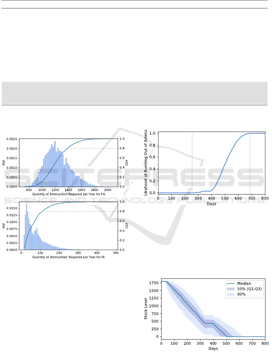
Table 2: Input parameters for Ammunition Type A demand for FG (unshaded rows) and FE (grey-shaded rows).

Name Frequency (per year) When Quantity Duration (in days)

Ex Group 1 DISCRETE(1:0.8, 2:0.2) UNIFORM(32;335) TRIANGULAR(45;90;180) 14

Ex Group 2 DISCRETE(1:0.8, 2:0.2) UNIFORM(32;335) TRIANGULAR(45;90;150) 14

Ex Group 3 DISCRETE(1:0.8, 2:0.2) UNIFORM(32;335) TRIANGULAR(30;60;120) 14

Ex Group 4 DISCRETE(1:0.8, 2:0.2) UNIFORM(32;335) TRIANGULAR(10;50;100) 14

Ex Group 5 DISCRETE(1:0.8, 2:0.2) UNIFORM(32;335) TRIANGULAR(45;60;90) 14

Ex Group 6 DISCRETE(1:0.8, 2:0.2) UNIFORM(32;335) TRIANGULAR(15;100;180) 14

Ex Group 7 0.125 UNIFORM(32;335) TRIANGULAR(20;30;40) 14

Ex Group 8 DISCRETE(1:0.8, 2:0.2) UNIFORM(32;335) TRIANGULAR(10;90;250) 14

Ex Group 9 0.5 UNIFORM(32;335) TRIANGULAR(30;90;135) 14

Ex Group 10 DISCRETE(1:0.8, 2:0.2) UNIFORM(32;335) TRIANGULAR(120;280;450) 14

Ex Group 11 0.125 UNIFORM(32;335) TRIANGULAR(10;20;30) 14

Ex Group 12 DISCRETE(1:0.8, 2:0.2) UNIFORM(32;335) TRIANGULAR(25;50;75) 14

Ex Group 13 DISCRETE(1:0.8, 2:0.2) UNIFORM(32;335) TRIANGULAR(40;50;60) 14

Op Type 1 DISCRETE(1:0.8, 2:0.2) UNIFORM(274;305) TRIANGULAR(10;25;62) TRIANGULAR(50;60;70)

Op Type 2 POISSON(0.1) UNIFORM(1;365) TRIANGULAR(30;48;65) TRIANGULAR(360;1080;1800)

Op Type 3 POISSON(0.125) UNIFORM(1;365) TRIANGULAR(40;80;200) TRIANGULAR(150;180;270)

Op Type 4 POISSON(0.125) UNIFORM(1;365) TRIANGULAR(20;60;100) TRIANGULAR(60;260;720)

conﬁrm that the majority of demand is generated from

FG (exercises) and that the annualized order quantity

should probably be greater than 1308.

Figure 2: Distribution of the demand per year for FG (top)

and FE (bottom).

3.3.2 Stock Level

A question often of interest to inventory management

practitioners is “How long can we expect the current

stock to last under various circumstances?” For exam-

ple, if no orders were made, how long would it take

before the stockpile is emptied? Figure 3 addresses

this question. It shows the CDF computed to illustrate

the likelihood that the stockpile will be emptied after

various time durations if no replenishment orders are

made. From this plot it is expected that with an initial

stock of 1,800 units, it would take between 253 and

686 days (indicated by dashed vertical lines) to reach

a stockout.

Figure 3: Stockout time of occurrence (1,000 replications).

To accompany Figure 3, Figure 4 depicts the evo-

lution in the distributions of stock level over time.

Shown are the median level, 10th-90th percentile lev-

els, and the 25th-75th percentile levels at each time

instant. (The latter of these percentile measures are

known as the ﬁrst and third quartiles, Q1 and Q3, re-

spectively.)

Figure 4: Stockpile level over time if no orders were made.

ICORES 2023 - 12th International Conference on Operations Research and Enterprise Systems

Another aspect of interest is how stock levels are

expected to vary if replenishment orders are placed.

Graphs like Figure 4 can be produced for each varia-

tion, where in this case individual variation represents

a unique combination of order frequency and order

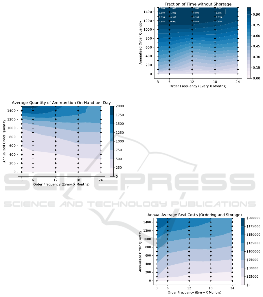
quantity. Alternately, a visualization that aggregates

expected results across all variations can be produced

as shown in Figure 5 where each “+” marker repre-

sents the result from a particular variation. The “+”

marker at the bottom left of the plot corresponds to

Variation 1 while the one at the top right corresponds

to Variation 80. The contours in this plot facilitate the

characterization of average stock levels across all 80

variations in a single graph.

Figure 5: Contour plot showing the average number of am-

munition on-hand per day for all 80 variations.

3.3.3 Supply vs Demand Performance

An ability to assess how well the ammunition sup-

plies are expected to meet the demand is important

if the long term performance of a particular stock-

piling scheme is to be determined. An associated

question posed by an inventory management practi-

tioner might be: “If implemented, how well do each

of the potential combinations of order quantity and or-

der frequency meet the estimated demand?” Several

performance measures can be considered to address

this question. One measure is the fraction of activi-

ties (i.e., exercises and operations) for which all de-

mands could be fulﬁlled from available stock. A sec-

ond measure is the fraction of simulation time over

which there are no ammunition shortfalls. An exam-

ple result showing the latter measure is presented in

Figure 6. Again, in this contour plot, the “+” mark-

ers represent the 80 variations. For illustrative pur-

poses white annotations are added to variations with

a fraction above 0.95. There are 16 variations in this

notional case study associated with a level above this

threshold.

Figure 6: Contour plot showing the fraction of time without

shortage for all 80 variations.

3.3.4 Cost

When choosing a good combination of order quantity

and order frequency, costs can be an important fac-

tor. As discussed earlier, the cost can be characterized

by various types in FEAST, i.e., storage cost, order-

ing cost and penalty cost. The user can drill-down or

aggregate-up to better understand the costs associated

with the combinations. Here we focus only on “real

costs” which are represented as the summation of or-

dering and storage costs. The average annual average

real costs for Variations 1 through 80 are shown in

Figure 7. As shown in this ﬁgure, the most expensive

variations (with costs greater than $150,000 per year)

are 14, 15, 16, 31 and 32.

Figure 7: Contour plot of the real costs (storage and order-

ing) for all 80 variations.

3.3.5 Cost vs Performance

The graphs and statistics shown thus far for our case

study are descriptive in nature, i.e., they illustrate

some of the basic information that can be gleaned

from FEAST. However, they can also aid in the pro-

vision of more in-depth analyses and provide insights

A Simulation Tool for Exploring Ammunition Stockpile Dynamics

to support decision-making.

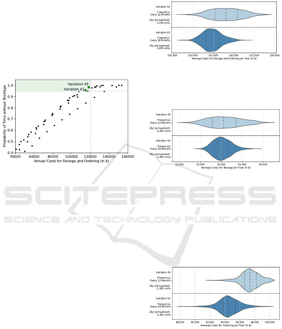
For example, assume that an average annual bud-

get of $120,000 is speciﬁed for Ammunition Type A,

and that the desired fraction of time without shortage

is set at 0.95. Figure 8 graphs real costs as a function

of the fraction of time without shortage. The markers

in this plot represent the variations tested in our case

study. The green-shaded area, delimited by Cost ≤

$120,000 and Time Without Shortage ≥ 95%, corre-

sponds to the region where both criteria are satisﬁed.

Figure 8: Scatter plot of the costs as a function of time with-

out shortage for all 80 variations.

Such graphs provide a basis for quickly compar-

ing variations and help to demarcate good options that

could be investigated in more detail. For our test case,

two viable variations exist within the shaded region

of Figure 8, i.e., Variation 45 (12 month ordering in-

terval and annualized order quantity of 1,200 units)

and Variation 61 (18 month ordering interval and an-

nualized order quantity of 1,200 units). These could

be further explored by an interested inventory man-

agement practitioner before one is selected for imple-

mentation.

3.3.6 Further Analysis

Once promising options like Variations 45 and 61 are

identiﬁed from Figure 8, more speciﬁc analysis can

be conducted. For example, from Figure 7, the av-

erage annual real costs for Variations 45 and 61 are

$118,187 and $114,757, respectively. Figure 9 illus-

trates the distribution of these annual real costs for the

two variations. Also shown in Figure 9 are the 25th a

75th percentiles of these cost distributions. From this

graph Variation 61 appears to be the less expensive of

the two options, with its median being located outside

of the region encompassing the 25-75th percentiles of

Variation 45.

For purposes of further investigation, Figure 10

shows the distribution of annual storage costs for each

of the two variations. Although the shapes of the dis-

Figure 9: Violin plots comparing the distribution of the av-

erage yearly costs for storage and ordering over the 1,000

replications for Variations 45 and 61.

tributions are slightly different, the storage costs for

both variations appear to be quite similar.

Figure 10: Violin plots comparing the distribution of the

average yearly costs for storage over the 1,000 replications

for Variations 45 and 61.

Figure 11 illustrates the distribution of average an-

nual ordering costs for both variations. Visual assess-

ment leads to the conclusion that signiﬁcant differ-

ences in the real costs for the two variations results

from differences in ordering costs. This can be ex-

plained from by the fact that there is a nontrivial ﬁxed

cost associated with each order regardless of the order

quantity, and more orders are made with Variation 45

than with Variation 61.

Figure 11: Violin plots comparing the distribution of the

average yearly costs for ordering over the 1,000 replications

for Variations 45 and 61.

The notional case study in this section illus-

trates some of the functionalities of FEAST, how-

ever FEAST has additional features not demonstrated

here (see Section 2). A practitioner is afforded rather

wide ﬂexibility to rerun the simulation with differ-

ICORES 2023 - 12th International Conference on Operations Research and Enterprise Systems

ing dynamics or alternate parameter settings. For ex-

ample additional budget constraints could be added,

additional logic could be introduced to represent the

behavior of multiple stockpiles, and other ammuni-

tion natures could be incorporated. Additional post-

processing scripts can also be composed.

4 LIMITATIONS AND

EXTENSIONS

A key limitation of FEAST is elements are consid-

ered independently, so common constraints or possi-

ble ammunition substitutions are not accounted for.

For example, artillery ammunition is complex (Pond

and Pittman, 2020) and is comprised of four compo-

nents (fuse, primer, propellant, and projectile)—all of

which are required and so cannot be modelled as inde-

pendent. Likewise, possible concurrency constraints

on operations are not imposed by FEAST despite

Canada’s defence policy explicitly providing concur-

rency expectations (Department of National Defence,

2017).

Incorporation of dependencies such as dependent

components, substitutional relationships, priorities on

usage, considering natures from a capabilities lens,

etc. are complex concerns that would be difﬁcult

to incorporate in FEAST’s inherently independent

framework. Despite this difﬁculty some progress can

be made. For example, FEAST has been built such

that demands can be externally generated and used as

input to FEAST. This feature enables concurrency

constraints to be imposed by an external, specialized,

program, and we will be exploring ingesting opera-

tion schedules generated by Force Structure Readi-

ness Assessment (FSRA), a Monte Carlo tool that in-

corporates CAF’s FE and platform deployment con-

straints (Dobias et al., 2019).

Contrariwise to FEAST ingesting demand gener-

ated elsewhere, demand generated by FEAST can be

used to feed other tools. For example, by binning

FEAST output, the demand on discrete time periods

could be used as input for an ADP model for the pur-

pose of generating improved ordering policies. While

stockpile capacity constraints and order lead times

make the simple unconstrained, immediate delivery

ADP formalism for stockpiles (Powell, 2009) inap-

propriate one can incorporate these factors and mod-

ify the formalism appropriately.

As the event set is fundamental to DES we re-

mark on potential efﬁciency gains. FEAST leverages

Python’s heapq (Python documentation, 2022) to im-

plement the event set as a priority queue, which has

O(log(n)) insert and remove costs. Note that sorting

n numbers can be achieved by inserting and removing

into an event set; as sorting has known O(n log(n))

bound this suggests that improved insert or remove

costs may be achievable. Indeed, pairing heaps (Fred-

man et al., 1986) have theoretical O(1) insert costs

and retain O(log(n)) removal costs and thus achieve

the efﬁciency bound in a tighter fashion. Importantly,

pairing heaps and related rank pairing heaps are em-

pirically demonstrated to be efﬁcient in practice, even

under adversarial testing (Stasko and Vitter, 1987;

Fredman, 1999). As heaps are abstract data structures

where implementation is hidden behind an interface,

switching the implementation is feasible in FEAST

with minimal changes to the code required.

Proﬁling results indicate Pandas and Python book

keeping operations, such as iterating through vi-

gnettes and copying objects, are dominant costs and

the event set contributes little to the total cost. For

example, insert and remove off the event set made

up roughly 5% of the computational costs of the in-

ner simulate module, for the scenarios we consider

here. For context regarding computational speed, to-

tal computations run on an order of minutes, for 1,000

replications of our single variant scenarios. The evi-

dence suggests mild efﬁciency gains can be achieved

by moving to a pairing heap implementation, and that

this gain will make up a larger fraction of the to-

tal if some refactoring of the Python code is made

to reduce costly approaches—for example, one ini-

tial trial change to reduce copying objects reduces

FEASTs bookkeeping costs such that the event set

makes closer to 10% of the total cost. As such, tri-

aling pairing heap or related heaps (Haeupler et al.,

2009; Stasko and Vitter, 1987) in FEAST, in combi-

nation with judicious code changes in FEAST itself,

constitutes practical follow on work that we will con-

sider in more detail.

5 CONCLUSION

FEAST is a DES model developed by DRDC CORA

to help practitioners within DND and the CAF ex-

plore questions regarding the supply, demand and re-

plenishment dynamics associated with ammunition.

The FEAST simulation engine has been implemented

in the Python programming language. Inputs and

outputs are managed using Microsoft Excel and ﬂat

comma separated value ﬁles. Stochastic demands for

ammunition are generated from lists of potential mil-

itary exercises and operations. Ordering and resupply

policies, which also incorporate stochastic variables,

are speciﬁed as inputs. Supply versus demand, tem-

poral dynamics and ﬁnancial considerations can be

A Simulation Tool for Exploring Ammunition Stockpile Dynamics

explored with FEAST. The tool is ﬂexible allowing

the user to quickly answer “what if” type questions.

In this paper, we provided an overview of FEAST and

demonstrated certain functionalities by way of a no-

tional case study consisting of independent demands

for the same type of ammunition from 13 military ex-

ercises and 4 military operations. The case study ex-

plored 80 resupply options, several of which were vi-

sualized and highlighted via post-processing of sim-

ulation outputs. Areas for extension and improve-

ment of FEAST include adding features so that: am-

munition substitutions and compositional dependen-

cies can be modelled; outputs from other Monte Carlo

models used by DND and the CAF can be ingested as

FEAST inputs; and improvements to computational

performance can be realized.

ACKNOWLEDGEMENTS

The authors would like to thank Mr. R

emi Gros-Jean

for his contribution and, in particular, for developing

FEAST in the Python programming language which

resulted in a solid and clean implementation. At the

time, Mr. Gros-Jean was a co-op student from the

University of Ottawa, Canada, employed in DRDC

CORA.

REFERENCES

Andrews, W. and Hurley, W. (2004). Approaches to deter-

mining army operational stockpile levels. Canadian

Military Journal, 5(2):37–46.

Bacot, R. (2009). Global movements and operational sup-

port hub concept: Global reach for the Canadian

Forces. The Canadian Air Force Journal, 2(3):8–17.

Brown, J. (2008). Conventional ammunition in surplus: A

reference guide. Small Arms Survey.

Department of National Defence (2017). Strong, Secure,

Engaged: Canada’s defence policy.

Devroye, L. (1998). Non-uniform random variate genera-

tion. Springer, London, 2nd edition.

Dobias, P., Hotte, D., Kampman, J., and Laferriere, B.

(2019). Modeling future force demand: Force Mix

Structure Design. In Proceedings from the 36th In-

ternational Symposium on Military Operational Re-

search. ISMOR.

Fredman, M. L. (1999). On the efﬁciency of pairing heaps

and related data structures. Journal of the ACM

(JACM), 46(4):473–501.

Fredman, M. L., Sedgewick, R., Sleator, D. D., and Tarjan,

R. E. (1986). The pairing heap: A new form of self-

adjusting heap. Algorithmica, 1(1):111–129.

Ghanmi, A. (2016). A stochastic model for military air-to-

ground munitions demand forecasting. In 2016 3rd

international conference on logistics operations man-

agement (GOL), pages 1–8. IEEE.

Guy, P. (2010). Strategic munitions planning in non-

conventional asymmetric operations. Technical re-

port, NATO C3 AGENCY THE HAGUE (NETHER-

LANDS).

Haeupler, B., Sen, S., and Tarjan, R. E. (2009). Heaps sim-

pliﬁed. arXiv preprint arXiv:0903.0116.

Nance, R. E. (1996). A history of discrete event simulation

programming languages. In History of programming

languages—II, pages 369–427.

Pond, G. and Pittman, J. (2020). Forecasting and costing of

a new 105mm modular propellant: In support of the

Royal Canadian Artillery regiment. In 2020 9th In-

ternational Conference on Industrial Technology and

Management (ICITM), pages 102–106. IEEE.

Powell, W. (2009). What you should know about approxi-

mate dynamic programming. Naval Research Logis-

tics, 56(3):239–249.

Python documentation (2022). heapq — heap queue algo-

rithm. https://docs.python.org/3/library/heapq.html.

Rempel, M. and Cai, J. (2021). A review of approximate dy-

namic programming applications within military op-

erations research. Operations Research Perspectives,

8:100204.

Stasko, J. T. and Vitter, J. S. (1987). Pairing heaps: ex-

periments and analysis. Communications of the ACM,

30(3):234–249.

Vershinin, A. (2022). The return of industrial warfare.

Royal United Services Institute (RUSI).

APPENDIX

Appendix A: Veriﬁcation in Steady-State

FEAST is highly ﬂexible. The ﬂexibility is required

to allow general “what if” questions to be asked which

is achieved at the cost of added complexity: as a re-

sult FEAST is approximately 1,500 lines of Python

code. As FEAST is intended to inform decisions, ver-

iﬁcation is important to increase conﬁdence that the

implementation works as intended. We consider var-

ious test cases to check features and critically assess

results. Here we present two related test cases.

Given the FG and FE vignettes to be simulated,

we can determine the expected annual demand under

steady-state conditions (i.e., distributions describing

frequencies, durations, and quantities are static over

time). For stochastically varying vignettes we note

that the expectation is simply the annual frequency

multiplied by the average quantity. An added nuance

occurs for “Op Type 2”, which, unlike other vignettes,

has multiple demands occurring over the operation.

In such cases, the overall demand is

D/Ie, where

Q is the average quantity demanded per interval,

ICORES 2023 - 12th International Conference on Operations Research and Enterprise Systems

is the average duration, and I is the sub-demand in-

terval. This holds, as demand in FEAST is modelled

as impulses that occur at the start of a demand period

and so d

D/Ie is the expected number of demands for

a vignette that has sub-intervals.

Another nuance in determining the expected an-

nual demand is that there are a mixture of stochasti-

cally occurring vignette demands, as well as vignettes

that occur with a ﬁxed frequency of 1 out of X years.

For example, “Ex Group 7” has a ﬁxed frequency of

0.125, or once every 8 years. The code is structured

such that, after an optional burn-in period, time starts

at zero, and so ﬁxed frequency vignettes will occur in

the ﬁrst year and reoccur every X years.

From the parameters in Table 2, supplemented

with “Op Type 2” having an interval of 360 days, we

can calculated the expected demand. As FEAST is

a DES implementation of a SP we know that, in re-

gions with ﬁxed parameters, ergodicity holds and the

average annual demand generated by the simulation

should match the calculated average. We can estimate

the standard error of the mean (SEM) as σ/

√

R, where

σ is the standard deviation of the measure (demand

here) and R is the number of replication-years.

We determine two cases to use as veriﬁcation

cases. For both we ﬁrst burn-in the simulation for ﬁve

years before collecting statistics to ensure that there

are no initial condition artifacts, as the vignette with

the longest duration (“Op Type 2”) can be up to al-

most ﬁve years long. In particular, note that we can-

not start the simulation with a vignette in progress and

therefore near t = 0 ergodicity does not hold; once

t > D

max

, where D

max

is the longest vignette duration,

ergodicity holds. After this burn-in we then consider:

1) a one year simulated period (where we know all

ﬁxed frequency vignettes will be active) where we de-

termine an expected annual demand of 1383.40, and

2) an “inﬁnite” year simulated period (where the ﬁxed

frequency vignettes will present their overall annual

average, i.e., 1/X) where we determine an expected

annual demand of 1306.68.

We ﬁx R = 10,000, so in case 1 we consider

10,000 replications and simulate for one year and in

case 2 we consider one replication and simulate for

10,000 years. For case 1 we ﬁnd that the average de-

mand is 1383.4 ±1.9, where we use the SEM to de-

termine precision. This has excellent agreement with

the expected value we calculate (1383.40), where the

strong agreement (better than estimated precision)

can be attributed to the ﬁxed frequency vignettes re-

ducing error over a purely stochastic case. For case

2 we ﬁnd that the average demand is 1307.7 ±2.0.

This also has excellent agreement with our calcu-

lated expected value (1306.68), and we attribute the

agreement within estimated precision to 1) the large

time interval indistinguishability between a ﬁxed fre-

quency event where events occur once every X years

and a stochastic (Bernoulli) process and 2) small ex-

pected correlation between samples, and so we expect

the SEM to be descriptive of the observed precision.

While veriﬁcation that the average annual demand

simulated by FEAST is equal to the expected value is

a simple test, it is a statistically exact one and there-

fore a strong test.

A Simulation Tool for Exploring Ammunition Stockpile Dynamics