Workforce Modelling with Experience Accumulation

Timo Lahteenmaa-Swerdlyk

, Franc¸ois-Alex Bourque

and Slawomir Wesolkowski

Centre for Operational Research and Analysis, Development Research and Defence Canada,

60 Moodie Drive, Ottawa, ON K1A 0K2, Canada

Royal Canadian Air Force, Department of National Defence, 101 Colonel By Drive, Ottawa, ON K1A 0K2, Canada

Keywords:

Discrete-Event Simulation, Mentoring, Population Dynamics, Population Model.

Abstract:

The purpose of this work is to investigate the population dynamics of on-the-job training in a military appli-

cation, a scenario where mentees enter the system to receive training under the supervision of mentors, before

becoming mentors themselves. This work builds on the two-level model which only considers the total mentee

(level 1) and mentor (level 2) populations. Accumulation of experience is used to denote training progression,

improving the tracking of mentees through their training. Two new models are considered: (1) A multi-stage

mentee training model, which sub-divides the training into stages the mentees must progress through, and

(2) A transport model, a limit case as the number of stages is increased to inﬁnity, resulting in a continuous

training medium mentees progress through. These two models are investigated by solving their respective an-

alytical models. To verify system behaviours, analytical solutions are compared to discrete-event simulations.

1 INTRODUCTION

For military occupations, an important aspect of pro-

fessional development is on-the-job training. In the

Canadian context, this takes the form of a system-

atic progression where personnel go through various

phases: they enter the system as mentees (e.g., ap-

prentices) and receive training under the supervision

of mentors (e.g., journeymen or masters), before be-

coming mentors themselves and productive members

of the workforce (Schaffel et al., 2021). To reduce

personnel costs while ensuring a necessary workforce

size and readiness, careful planning and modelling

must be undertaken on these training systems.

Bastian and Hall review approaches used in mili-

tary workforce planning and modelling (Bastian and

Hall, 2020). Prime examples of population dynam-

ics modelling include differential equations (Boileau,

2012; Vincent and Okazawa, 2019), Markov decision

models (Zais and Zhang, 2015; Diener, 2018; Su-

vorova et al., 2019) and system dynamics (Forrester,

1965) which utilizes continuous stocks and ﬂows as

well as feedback loops to examine how organizational

structure, policies and decisions interact. An exam-

ple of this last method was implemented to model

mentee-mentor dynamics for pilots (S

eguin, 2015).

Analysis of the composition of workforces as well

near-term projections of occupational requirements

also relied on statistical methods (Bryce and Hender-

son, 2020; Okazawa, 2020). Yet, the most common

approach is based on using discrete-event simulations

to track the progress of personnel through a military

training system (Novak et al., 2015; Henderson and

Bryce, 2019).

The military workforce population models usu-

ally capture only the upward rank ﬂow due to pro-

motion, not the experience accumulation due to the

mentee-mentor dynamics. A notable exception is a

system dynamics model which considers trainee pi-

lots and experienced pilots who mentor the trainees

eguin, 2015). In most of the research, the popu-

lation variables are continuous in order to generate

computationally-efﬁcient models that are easier to use

on large populations. These models are less accurate

when studying occupations with small populations.

This work builds on the two-level mentor-mentee

model derived from the ubiquitous “predator-prey”

model (Swift, 2002), which considers the total mentee

and mentor populations over time (Schaffel et al.,

2021). However, in this mentor-mentee model, indi-

vidual mentees cannot be distinguished from one an-

other in the total pool of mentees and thus a mentee

with minimal experience or time training as a mentee

may upgrade at any time to a mentor. Therefore, some

mentees may become mentors after completing only

a small amount of on-the-job-training, which is not

Lahteenmaa-Swerdlyk, T., Bourque, F. and Wesolkowski, S.

Workforce Modelling with Experience Accumulation.

DOI: 10.5220/0011620400003396

In Proceedings of the 12th International Conference on Operations Research and Enterprise Systems (ICORES 2023), pages 27-37

ISBN: 978-989-758-627-9; ISSN: 2184-4372

 2023 by His Majesty the King in Right of Canada as represented by the Minister of National Defence and SCITEPRESS – Science and Technology Publications, Lda. Under

CC license (CC BY-NC-ND 4.0)

realistic. Furthermore, the training progression of in-

dividual mentees is unclear as they form an indistin-

guishable pool from one another. In a realistic sce-

nario, mentees would accumulate experience through

their training. Modelling this experience accumula-

tion process allows for the tracking of the training

of each mentee in the system. Therefore, we intro-

duce a new experience accumulation mechanism to

resolve the issues encountered with the previous two-

level model.

In this paper, two new models are devised based

on the two-level model by dividing the total mentee

population into multiple stages to bin the training pro-

gression of mentees. First, we introduce a multi-

stage mentee training model that bins the mentee

pool into a generalized discrete number of stages,

forming a system of multiple ordinary differential

equations (ODEs). Second, we devise a “transport”

model, which is the result of increasing the number of

stages to inﬁnity, forming a partial differential equa-

tion (PDE). To verify the system dynamics of these

models, a discrete-event simulation (DES) of each

model is compared to their corresponding analytical

versions.

The remainder of this report is organized as fol-

lows. Section 2 gives an overview of the previously

introduced two-level model (Schaffel et al., 2021).

Next, Section 3 and Section 4 describe the multi-stage

and transport models respectively. In both instances, a

benchmark scenario is used to examine the analytical

solutions and corresponding DES’s are set up to ver-

ify the dynamics of each model. Section 5 compares

the analytical solutions of the three models discussed.

Finally, Section 6 concludes the paper.

2 TWO-LEVEL MODEL

In this section, the two-level mentor-mentee model

(Schaffel et al., 2021) is re-introduced. This model

considers the mentee and mentor populations to each

be a single pool of the corresponding type of person.

The previously described saturation effects (Schaffel

et al., 2021) are not considered, and the training ca-

pacity is assumed to be inﬁnite. The analytical equa-

tions for this model are described in Section 2.1. In

Section 2.2, a DES of the model is set up. Finally in

Section 2.3, the model is investigated with a bench-

mark scenario, which will be used throughout the pa-

per.

2.1 Analytical Model

The two-level model for an inﬁnite training capacity

is deﬁned as (Schaffel et al., 2021),:

˙x = a −bx (1)

˙y = bx −cy (2)

where x and y denote the mentee and mentor popula-

tions respectively, a is the intake rate of mentees into

the system, b is the upgrade rate of mentees to men-

tors, and c is the attrition rate of mentors. A mentee

will take an average of 1/b time units to upgrade to

a mentor, and a mentor will stay in the system for an

average of 1/c time units before leaving. The intake,

upgrade, and attrition rates are assumed to be con-

stant over time. For the model, the rate of change for

the mentee population ( ˙x) is equal to the intake rate

of mentees (a) minus the upgrade rate of mentees to

mentors (bx), while the rate of change of the mentor

population ( ˙y) is equal to the upgrade rate (bx) minus

the attrition rate of mentors (cy). In this model, the

fraction of the mentee and mentor populations chosen

to be upgraded or attrited is assumed to be propor-

tional to their respective sizes.

Solving the ODEs, the analytical solution is

shown in Eqn. (3) and Eqn. (4). The mentee and men-

tor populations decay exponentially from their initial

populations (x

and y

) to the target populations (x

and y

) of x

= a/b and y

= a/c respectively as time

(t) increases since the upgrade and attrition rates are

positive and real values. The system decays to the

target populations regardless of the size of the initial

mentee and mentor populations.

x(t) =x

+ (x

−x

−bt

(3)

y(t) =y

c −b

−x

−bt

(4)



−

c −b

−y

)



−ct

(5)

A drawback of this model is its inability to track

the progress of every mentee in the system (Schaffel

et al., 2021). The model only consists of two pools

for the mentees and mentors respectively. Once a

mentee is added into the mentee pool, it becomes in-

distinguishable from the other mentees in the system.

Since mentees cannot be distinguished from one an-

other and a constant proportion of the mentee pool is

always selected to upgrade, a mentee can be expected

to upgrade at any time. For example, a mentee could

be selected to upgrade after being added very recently,

staying in the mentee pool for a very small amount of

time, or a mentee could remain in the mentee pool

for a very large amount of time if it is never part

ICORES 2023 - 12th International Conference on Operations Research and Enterprise Systems

of the proportion of the population selected to up-

grade. Therefore, while the average training time for a

mentee is 1/b time units, a mentee can take anywhere

from zero to an inﬁnite amount of time to upgrade,

which is not realistic. Since a mentee may upgrade at

any time, there is no clear training progression for the

mentees to follow.

2.2 Discrete-Event Simulation

To verify the analytical equations, a DES of the two-

level model was set up. A Discrete-Event Simulation

permits the tracking of each mentee and mentor in the

system allowing for control and observance over the

simulation process and output. At each event within

the simulation, deﬁned processes may be triggered to

occur for a mentee or mentor, such as an addition or

attrition from the system, or an upgrade of a mentee

to a mentor.

To set up the simulation, mentees and mentors

were assigned a training time and a time to attrit,

randomly given from exponential probability distribu-

tions with means of 1/b and 1/c respectively (Schaf-

fel et al., 2021). A mentee would enter the system and

remain as a mentee for their assigned training time.

They would then upgrade to a mentor and further re-

main in the system for their assigned time until they

leave via attrition.

Another consideration of implementing a DES is

the handling of whole mentee and mentor popula-

tions instead of the continuously-variable populations

present in the analytical model. This is particularly

important when determining the intake procedure of

mentees into the system. In the analytical model, the

intake is a constant function over time (a). However,

this is not possible in a DES since individual mentees

(i.e., not fractions of a mentee) need to enter the sys-

tem at discrete points in time. Therefore, to replicate

the constant intake of the analytical model, the time

interval between when mentees enter the system was

randomly chosen, given by an exponential distribu-

tion with a mean of a (Schaffel et al., 2021). In the

current implementation, a mentee may enter the sys-

tem at any time while still maintaining the average

intake rate of a mentees per time unit.

Of note, because all holding and inter-arrival times

are exponentially distributed, this simulation models

a continuous-time Markov chain.

2.3 Results for a Benchmark Scenario

In the chosen benchmark scenario, the mentee and

mentor populations undergo a growth where their

populations are doubled. Transitioning from an initial

state (x

) to a target steady state (x

), the input

parameters are ﬁxed to the following values:

) = (25,100)

) = (50,200)

c = 0.05

The intake (a), upgrade (b) and attrition (c) rates are

assumed to be ﬁxed and not vary over time. There-

fore, a and b are calculated to reach the target popu-

lations:

a = cy

= 10

b =

= 0.2

From the deﬁned values, the system will transition

from initial mentee and mentor populations of 25 and

100 respectively, to target populations of 50 and 200.

To reach this target, 10 mentees must enter the sys-

tem on average each time unit, and each mentee will

require an average of 5 time units of training before

upgrading to a mentor. Finally, a mentor will stay in

the system for an average of 20 time units before ex-

iting the system.

Fig. 1 shows the statistics for the mentee (blue,

bottom curve) and mentor (green, top curve) popula-

tions from the DES model for 1000 experiments. The

mean of the two populations is given by the dashed

line, and the shaded region gives two standard devi-

ations of the results. The analytical solution is also

plotted with the benchmark scenario. The two popula-

tions begin at their initial values of 25 and 100 respec-

tively and decay exponentially to their ﬁnal values of

50 and 200. The analytical solution and the simulated

mean of the two populations lie on top of each other

for all time and are within two standard deviations of

the simulated results. The standard error near steady

state was found to be around 0.225 and 0.45 for the

mentee and mentor populations respectively. Since

the discrete model is a Poisson point process, the ex-

pected standard errors are

√

c and

√

b for the mentee

and mentor populations, which are roughly equal to

the values observed. Given this, we are conﬁdent the

discrete model is set up correctly and is producing ac-

curate results.

3 MULTI-STAGE MENTEE

TRAINING MODEL

In Section 2.1, it was noted that there is a lack of

training progression in the two-level model since the

mentees form an indistinguishable pool and may up-

grade at any time. In an attempt to resolve this issue,

Workforce Modelling with Experience Accumulation

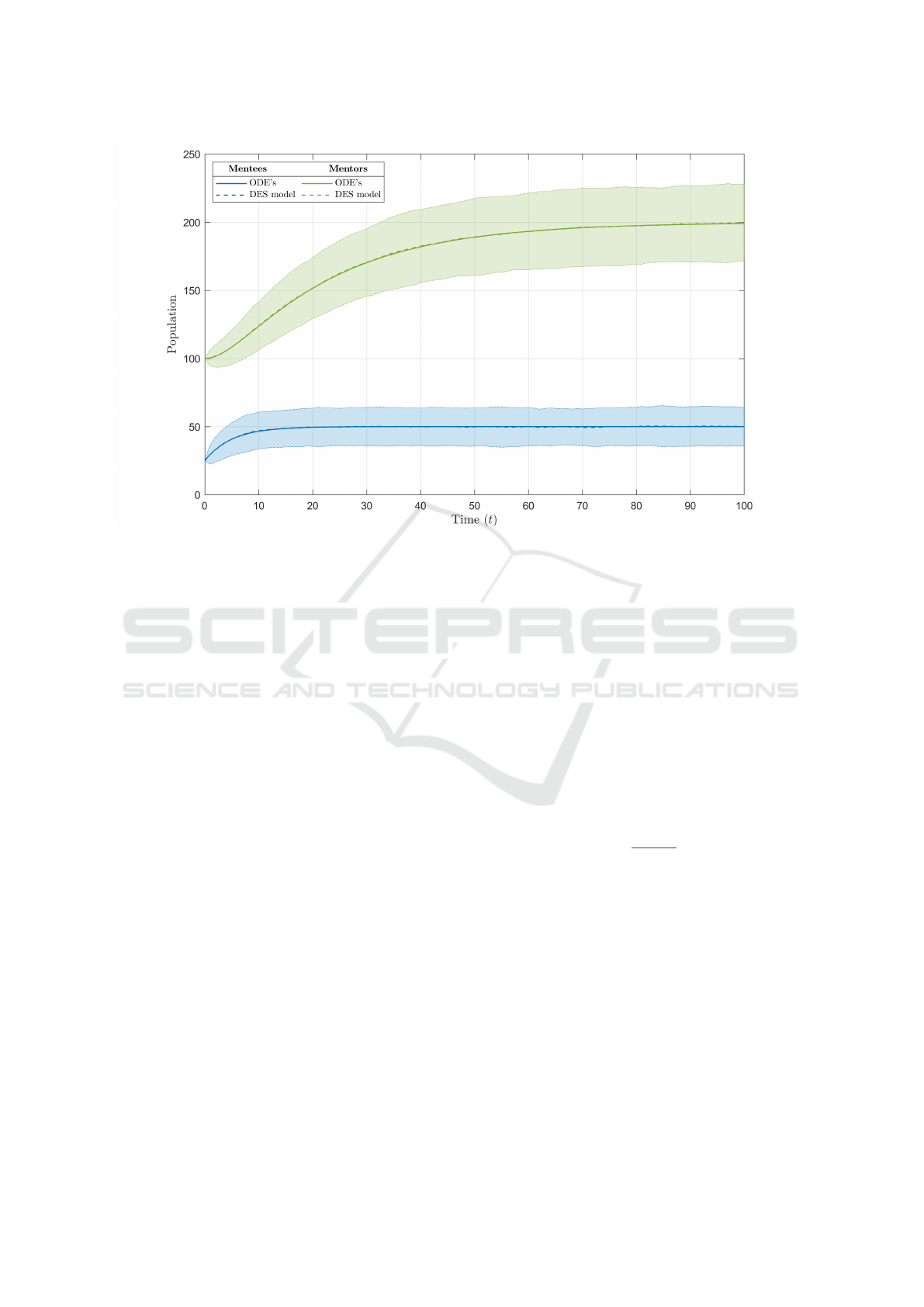
Figure 1: Analytical and DES implementations of the two-level model over time with the benchmark scenario.

the model was modiﬁed to split the mentee progres-

sion into multiple stages, which a mentee must pass

through to upgrade to a mentor. In this section, the

multi-stage mentee training model is introduced and

discussed. In Section 3.1, the analytical equations

for the multi-stage model are introduced, and in Sec-

tion 3.2, a DES implementation of the model is set

up. The results with the benchmark scenario are then

investigated in Section 3.3 for two scenarios: A ﬁve-

stage system and a 25-stage system.

3.1 Analytical Model

The system of equations for the multi-stage mentee

training model is shown as follows:

˙x

= a −bnx

˙x

= bn(x

−x

)

˙x

= bn(x

n−1

−x

)

˙y = bnx

−cy

(6)

where n denotes the number of mentee stages be-

fore upgrading to a mentor; and x

,··· , x

de-

note the mentee populations at each training stage

over time. In practical terms, the number of stages

is generally determined experimentally with a higher

number allowing us to model mentee training stages

with increasing granularity. The upgrade rate for

each mentee stage is proportional to the number of

stages in the system (nb) so that the total training time

through all the stages averages to 1/b. Like for the

two-level model, the fraction of the mentee popula-

tion chosen to upgrade from each stage is assumed to

be proportional to its total size. The mentor equation

remains the same as for the two-level model where its

rate of change is given by the difference in the men-

tors attrited and the mentees upgraded from the ﬁnal

stage. Finally, we will assume that the initial mentee

populations are evenly distributed between the stages.

Therefore, each stage will have an initial population

of x

/n.

The solution of the multi-stage analytical model is

as follows:

x(t) = e

−nbt

∑

j=1

∑

i=1

j−i

( j −i)!

+ e

−ct

+ x

(7)

The solution, x(t), is a column vector containing the

populations over time of the individual mentee stages

and the mentor population:

x(t) =







(t)

y(t)







(8)

The solution contains one degenerate eigenvalue,

−nb, with a multiplicity of n, a second distinct eigen-

value, −c, and a constant particular solution, x

. The

ICORES 2023 - 12th International Conference on Operations Research and Enterprise Systems

particular solution is the following column vector de-

noting the steady state values of each population:













(9)

For the generalized eigenvectors of the degener-

ate eigenvalue, v

, of length n + 1, its elements

1i,1

1i,2

,··· , v

1i,n+1

) are all zero except for the fol-

lowing:

1i,n−i+1

c −nb

(nb)

1i,n+1

(nb −c)

i−1

The eigenvector corresponding to the distinct eigen-

value of length n + 1 (the mentor solution) has the

following form:













(10)

Finally, the constants in the solution have the follow-

ing values:



−x



(nb)

c −nb

(11)

= y

−y

−

∑

j=1

(nb −c)

j−1

(12)

3.2 Discrete-Event Simulation

To set up a DES implementation of the multi-stage

mentee training model, the two-level discrete model

from Section 2.2 was modiﬁed so that the training for

a mentee was repeated n times to replicate the pro-

gression through each stage. For each repetition, a

mentee was assigned a training time given randomly

by an exponential probability distribution with a mod-

iﬁed mean of 1/nb. A mentee would enter the sys-

tem and remain in the ﬁrst stage for their ﬁrst as-

signed training period before upgrading to the second

stage. This process would repeat n times, simulating

a progression through each stage, until the mentee up-

graded to a mentor. Even with this modiﬁcation, the

overall simulation remains markovian.

One consideration faced with implementing a

DES was the handling of whole mentee populations to

determine the initial number of mentees at each stage.

For example, in a system with 10 mentee stages and

25 initial mentees, each stage would need to be pop-

ulated with 2.5 mentees to have an even distribution.

This is possible in the analytical model as the mentee

and mentor populations are continuous; however, this

cannot be done in a discrete implementation. To solve

this issue, the number of initial mentees at each stage

was randomly drawn from a discrete uniform distri-

bution with values between 1 to n. Therefore, given

enough experiments, the average distribution of initial

mentees should be even across all of the stages.

3.3 Results for the Benchmark Scenario

Fig. 2 shows the statistics for systems with 5 and 25

stages over time with the benchmark scenario. In both

cases, their respective DES simulations were run for

1000 experiments. Fig. 2a and Fig. 2c show their total

mentee and mentor populations over time. The mean

of the two populations is given by the dashed line,

and the shaded region gives two standard deviations

of the results. Fig. 2b and Fig. 2d show the population

of each stage over time with the dashed line indicat-

ing the mean. For all plots, their respective analytical

solutions are also plotted as solid lines in the same

colour.

From Fig. 2a, the mentee and mentor populations

are set initially at 25 and 100 respectively, and de-

cay exponentially to their target populations of 50

and 200. Compared to the two-level solution given in

Fig. 1, the mentee population for ﬁve training stages

decays quicker to steady state. Furthermore, the lower

number of mentees upgraded each time causes the

mentor population to spend more time near its ini-

tial population before beginning its exponential de-

cay. From Fig. 2b, each stage begins at its initial pop-

ulation of ﬁve mentees, then decays exponentially to

the same steady state populations of 10. It was ob-

served that each stage acts on the behaviour of the

previous stage: Stage 1 decays ﬁrst, then Stage 2, up

to Stage 5 which decays to steady state last. This was

interpreted as a progression of mentees through the

training stages: Mentees entering the system enter at

stage 1 ﬁrst, undergo training then upgrade to stage 2,

which gives an increase in the population of the sec-

ond stage. These mentees undergo training and up-

grade to stage 3, giving a population increase in stage

3. This process continues up the stages and into the

mentor population as mentees progress through the

system.

From Fig. 2d, each training stage begins at its

initial population of one mentee and decays expo-

nentially to the same steady state populations of two

mentees. Similar to a system with ﬁve stages, given

in Fig. 2b, each stage begins its decay in subsequent

order. However, the solutions decay to steady state

at a quicker rate and are much more bunched up in

Workforce Modelling with Experience Accumulation

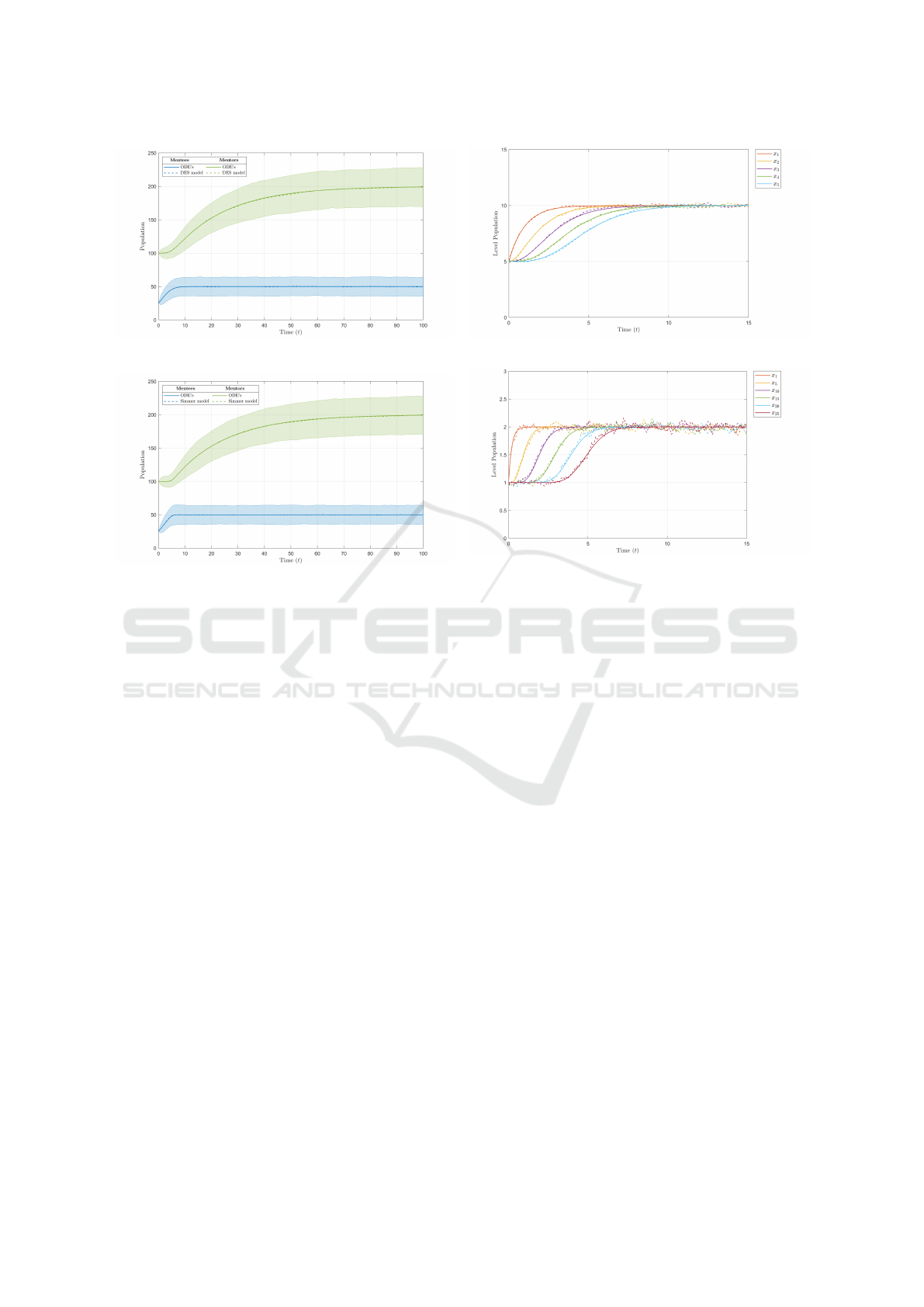
(a) Total mentee and mentor populations for ﬁve stages.

(b) Individual training stage populations for ﬁve stages.

(d) Individual training stage populations for selected stages

for 25 stages.

Figure 2: Analytical and DES implementations of the multi-stage model over time with the benchmark scenario. Total mentee

and mentor populations for (a) ﬁve stages; and (c) for 25 stages; and corresponding individual training stage populations for

(b) ﬁve stages; and (d) a sub-set of 25 stages.

time. This translates to the total populations given in

Fig. 2c, in which the decay to steady state for the to-

tal mentee population is also increased. The solutions

are more bunched up since the average time to steady

state for the total mentee population must still be 1/b

time units.

For all plots, the analytical solutions and the simu-

lated means of the populations lie on top of each other

and are within two standard deviations of the simu-

lated results. The standard error for the total popula-

tions near steady state was also identical to the val-

ues from the two-level model (0.225 and 0.45 for the

mentee and mentor populations respectively). The

standard error for the individual stages near steady

state was found to be around 0.1 and 0.045 for the

ﬁve- and 25- stage models respectively. These are

commensurate to the standard error of the total popu-

lation. Given this, we are conﬁdent the discrete mod-

els are set up correctly and are producing accurate re-

sults. Finally, it was noted that the population mean

of the individual mentee stages became noisier as the

number of stages is increased. This is believed to re-

sult from an ampliﬁcation of the discrete effects of

the model since the population size for the individual

stages decreases as more stages are added.

Overall, an improvement was observed over the

two-level model, in which there is now some form

of progression as mentees must pass through several

trackable stages. However, a similar drawback as the

two-level model is still present: The same proportion

of each stage is always selected to upgrade (nb), so a

mentee could be selected to upgrade to the next stage

at any time.

4 LIMIT CASE: TRANSPORT

MODEL

From Section 3.3, it was noted that a multi-stage

model showed some form of workforce progression

as mentees must pass through several stages of train-

ing before upgrading to mentors. However, each stage

suffered from the same issues as the two-level model,

as the mentees in each stage still could not be tracked

and may upgrade at any time. Therefore, in an at-

tempt to obtain the smallest interval of training which

could be tracked, the number of stages was increased

to inﬁnity, yielding a transport model. In this section,

this transport model is investigated and discussed. In

ICORES 2023 - 12th International Conference on Operations Research and Enterprise Systems

Section 4.1, the analytical equations for the transport

model are introduced, and in Section 4.2, a discrete

implementation of the model is set up. In Section 4.3,

the model is investigated with the benchmark sce-

nario.

4.1 Analytical Model

Two key issues arose when deriving the transport

model: (a) For an inﬁnite number of stages, each stage

must contain zero mentees on average to avoid a pop-

ulation of inﬁnity, and (b) Each mentee requires an

average upgrade time of zero time units through each

stage to avoid having an inﬁnite training time. To

solve these issues, the stages were redeﬁned a contin-

uous medium (l) and assigned an arbitrary total length

of one. For the new training regime, a mentee enters

the system at l = 0 and begins ﬂowing through the

medium undergoing training. Once a mentee reaches

l = 1, they upgrade to a mentor. The variable of

interest was also changed to the density of mentees

throughout the medium (u), which is more appropri-

ate for a continuous medium. The mentor equation

was modiﬁed to accommodate the use of density (u)

instead of a population size (x): the rate of change of

the mentor population is given by the difference in the

mentors’ attrition and the mentees exiting the medium

at l = 1.

The system of equations for the transport model is

deﬁned as:

∂

u(l,t) = −b∂

u(l,t) (13)

˙y = bu(1,t)−cy. (14)

The PDE for the mentee population was derived from

the multi-stage model, Eqn. (6).

For the initial condition of the PDE (u

), it was as-

sumed that the initial mentee density was evenly dis-

tributed throughout the medium. For the boundary

condition (u

), the density is ﬁxed to the ratio between

the intake rate (a) and the progression rate through the

medium (b) as given by:

. (15)

The boundary condition is assumed to turn on after

t = 0, preventing a conﬂict with the initial condition.

From (Novozhilov, 2020; Ko, 2020), the solution

of the transport PDE is given by the piecewise func-

tion:

u(l,t) =

(

if t ≤

if t >

(16)

The density across the medium begins at the initial

density (u

) and jumps up to the ﬁnal density (u

) at

the contour: l = bt.

To determine the analytical solutions for the total

mentee and mentor populations, the mentee solution

given in Eqn. (16) was rewritten using a Heaviside

step function:

u(l,t) = u

+ (u

−u



t −



, (17)

where H denotes the left-continuous Heaviside step

function, H(0) = 0. Using this representation, the

total mentee population was found by integrating

the mentee density across the medium, given by:

Eqn. (18).

x(t) = u

−b(u

−u

)





t −



−t



, (18)

where R denotes the ramp function. The solution

for the mentor population was found by substituting

Eqn. (17) into Eqn. (14) and solving the resulting

ODE. The equation for the mentor population is thus

given by:

y(t) = y

−ct



1 −e

−ct



−

−ct

−u

)



−e





t −



. (19)

4.2 Discrete-Event Simulation

To set up a DES implementation of the transport

model, the two-level discrete model from Section 2.2

was modiﬁed so that the training time for the mentees

is constant at 1/b instead of being drawn from an ex-

ponential distribution. This feature makes the simula-

tion non-markovian. To mimic an even distribution of

initial mentees throughout the medium (l), the initial

mentees were assigned a uniformly-distributed train-

ing time between zero and 1/b. This method repli-

cates the analytical system since all mentees progress

through the medium at a constant rate (b); therefore,

the initial position of a mentee along the medium was

inversely proportional to their training time.

4.3 Results for the Benchmark Scenario

To utilize the benchmark scenario with the transport

model, the initial and boundary conditions were ﬁxed

to the following values:

= 25

= 50.

With these deﬁnitions, the total mentee population,

found by integrating the mentee density over the

medium, still has an initial population of 25 mentees

and a ﬁnal population of 50.

Workforce Modelling with Experience Accumulation

For the DES, the density of mentees must be cal-

culated from the mentees present in the system over

time and their respective progression through their

training. Since mentees progress through the medium

at a constant rate, the location of a mentee in the

medium at a point in time can be inferred from their

training time (initial mentees) or arrival time into the

system (added mentees). To generate a surface plot

of mentee densities, mentees were binned together in

time and medium intervals. The bin in time was cho-

sen to be an interval of 1/12 time units, potentially

simulating a progression through the medium once

every month. The bin in the medium was chosen to be

1/60, matching the time interval so a mentee would

progress forward by one bin in the medium every time

interval.

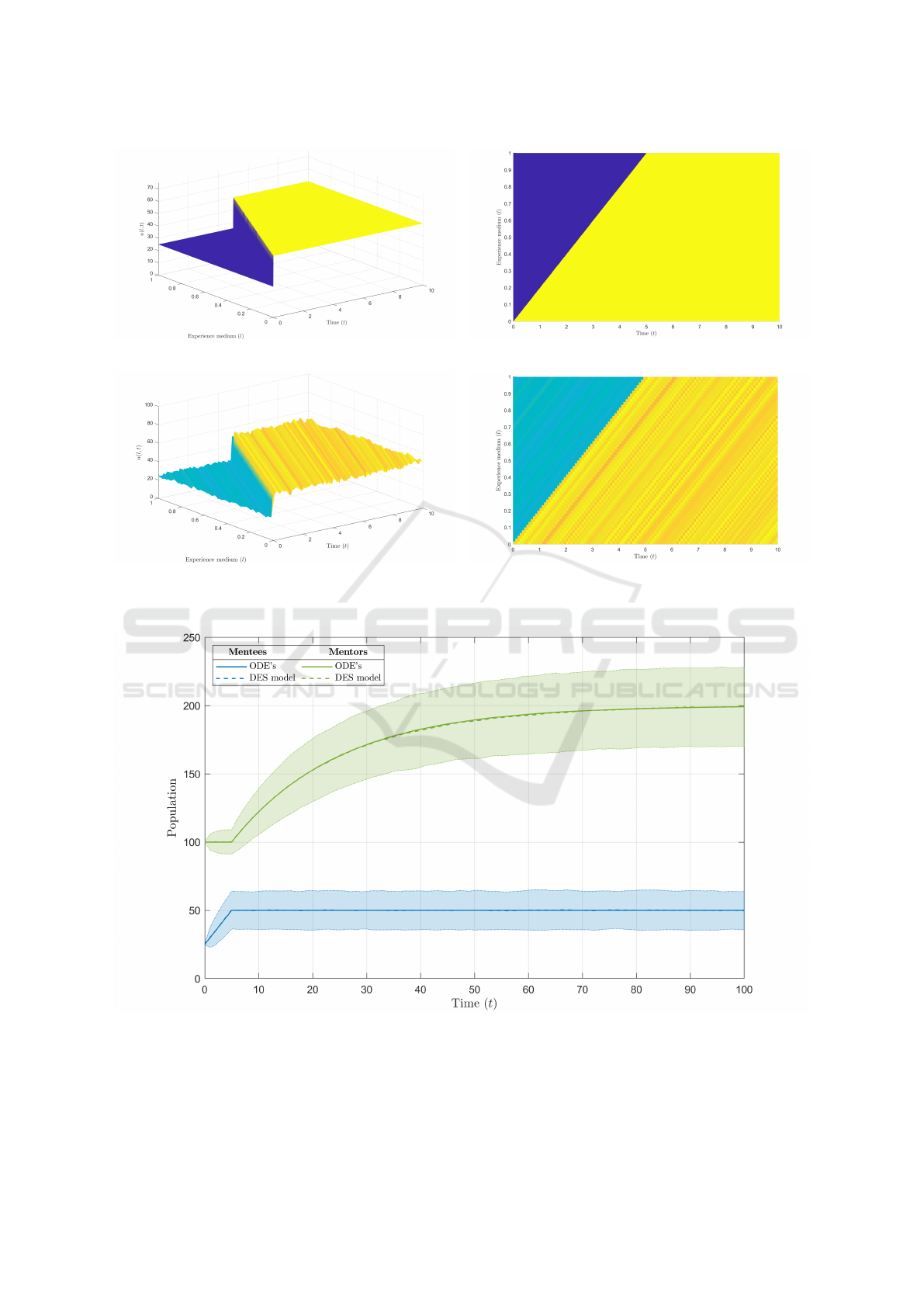
4.3.1 Surface Solution of the Mentee Population

Across the Medium

Fig. 3 shows the surface plot of densities for the an-

alytical PDE and DES with the benchmark scenario.

The simulation was run for 1000 experiments. From

the analytical solution, Fig. 3a and Fig. 3b, the den-

sity of mentees through the medium jumps from 25 to

50 after the contour l = bt. After 5 (1/b) time units,

the entire medium is populated at the ﬁnal density.

From (Novozhilov, 2020; Ko, 2020), the trans-

port PDE models a constant progression through the

medium at a rate of b. This gives straight-line con-

tours with a slope of b, as seen from the top-down

view in Fig. 3b. Therefore, in the transport model

each mentee has the same training time of 1/b. This

is different from the two-level and multi-stage models

given in Section 2 and Section 3, in which the training

time for mentees was exponentially distributed. This

constant training time between the mentees arises be-

cause as the number of stages is increased to inﬁnity

(n → ∞), the average time a mentee spends in each

stage approaches zero. For an average time of zero

in each stage, there must be no variance between the

training times for each mentee in the system, giving

the same training time for each. Finally, the loca-

tion of a mentee along the medium denotes how far

along they have progressed with their training. This

improves the tracking of mentees through their train-

ing as now a continuous medium is used to denote

their progression.

For the simulation output, Fig. 3c and Fig. 3d,

the initial density of mentees across the medium is

even around 25, and the ﬁnal density is even around

50. The surface plot also demonstrates nearly identi-

cal behaviour to the analytical solution, in which the

spike in density up to 50 occurs along the contour:

l = bt. From the top-down view, mentees progress

through the medium at a constant rate of b, like in

the analytical model. Given the similarities observed

between the analytical and discrete outputs, it is be-

lieved that the two versions of the transport model are

equivalent.

4.3.2 Solution of the Total Mentee and Mentor

Populations

The solutions for the total mentee and mentor pop-

ulations for the benchmark scenario are plotted in

Fig. 4. The analytical solutions given by Eqn. (18)

and Eqn. (19) are plotted as solid lines. The statistics

of the total populations from the DES model are also

plotted. The mean of the two populations is given

by the dashed line, and the shaded region gives two

standard deviations of the results. The mentee pop-

ulation linearly increases from the initial population

of 25 mentees to the ﬁnal population of 50. After 5

(1/b) time units, all initial mentees have upgraded to

mentors and the mentees now populate the system at

the ﬁnal density. Therefore, the mentee population

reaches steady state at this time. The mentor popula-

tion still undergoes its exponential decay at a rate of c.

However, the decay only begins once the mentee pop-

ulation reaches steady state and the incoming mentors

are at the ﬁnal density. The analytical solution and the

mean of the simulation results of the two populations

lie on top of each other, are within two standard de-

viations of the simulated results, and their standard

errors were found to be identical to the values from

the previous models (0.225 and 0.45 for the mentee

and mentor populations respectively). This gives fur-

ther conﬁrmation that the two versions of the transport

model are equivalent and the discrete model was set

up correctly.

5 COMPARISON BETWEEN THE

THREE MODELS

Fig. 5 shows the analytical solutions of the two-level

(one mentee stage), ﬁve- and 25- mentee stage, and

transport models plotted together with the benchmark

scenario for comparison.

From Fig. 5a, as the number of mentee stages is

increased, the decay rate of the ﬁnal population in-

creases. The transport model, shown in blue, is the

limit case, in which there is an inﬁnite decay rate and

simply reaches the ﬁnal population at 5 (1/b) time

units. From Fig. 5b, the exponential rise into the de-

cay to steady state for the mentor population also be-

comes sharper as the number of stages is increased.

Due to the varying sharpness in the rise, all solutions

ICORES 2023 - 12th International Conference on Operations Research and Enterprise Systems

(a) 3-D view, analytical PDE.

(b) Top-down view, analytical PDE.

(d) Top-down view, discrete simulation.

Figure 3: Surface plot of analytical and DES densities of the transport model.

Figure 4: Mentee and mentor populations over time for analytical and DES implementations of the transport model with the

benchmark scenario.

cross over each other as they decay to steady state at

the ﬁnal population of 200 mentors. From Fig. 5b at

20 time units, the two-level model, shown in purple,

has the lowest mentor population and is the furthest

from the steady state value, while the transport model

has the highest population and is the closest to the

Workforce Modelling with Experience Accumulation

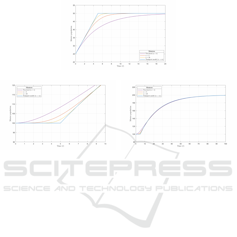
(a) Mentee population.

(b) Mentor population, zoomed in. (c) Mentor population, full decay.

Figure 5: Comparison of the analytical solutions of the two-level (one mentee stage), multi-stage (ﬁve and 25 mentee stages),

and transport models.

steady state value. Therefore, while all solutions have

the same decay rate (c) and a time to steady state of

inﬁnity, if a threshold value is used to denote the sys-

tem is at steady state, the transport model will always

have the quickest time to steady state, and the two-

level model will always be the slowest.

6 CONCLUSION

In this paper, the workforce population dynamics of

on-the-job training was investigated, building upon a

two-level model of the system given in (Schaffel et al.,

2021). In an effort to obtain a more realistic model,

two types of experiments were investigated: A multi-

stage model and a transport model. The analytical

solutions of these three models were investigated us-

ing a benchmark scenario in which the mentee and

mentor populations were doubled. The analytical so-

lutions and the model behaviours were veriﬁed using

a DES.

A drawback of the two-level model is that the

mentees are grouped in a pool and are indistinguish-

able from one another. A mentee could be expected to

upgrade to a mentor at any time, which is not realis-

tic and resulted in a lack of clear training progression

for each mentee. For the multi-stage model, some

training progression was observed as the population

of the individual stages changed over time. However,

each stages still suffered from the same issues as the

two-level model. The transport model was the limit

case of the multi-stage model as the number of stages

was increased to inﬁnity, in an attempt to track the

smallest portion of the mentee population which was

possible. In this system, all mentees had a constant

training rate. The tracking of mentees through their

training was greatly improved since their progression

was now represented by a continuous medium.

The transport model is essentially a pair of queues

in parallel where: (1) the mentee queue has a constant

service time to simulate a constant training rate, and

(2) the mentor queue has an exponentially distributed

service time to model attrition. This solves several is-

sues contained in the other two models: the mentees

in the transport model are much easier to track since

they will all progress through the medium at the same

rate, and only depart the mentee population once the

full medium is crossed, leading to a constant training

time. However, the equal training time and progres-

sion for all mentees in the system may not be realis-

tic. The mentor population is also still represented by

ICORES 2023 - 12th International Conference on Operations Research and Enterprise Systems

the same equation as the two-level model, which may

not be an accurate representation of a realistic sce-

nario when combined with the PDE for the mentee

population. Despite these issues, the formulation of

a transport model for the training scenario provides

a more ﬂexible and less complicated means of mod-

elling the progression of mentees to mentors than the

multi-stage model. This may aid in building up and

investigating more realistic workforce system imple-

mentations in the future. It is believed that a transport

model could be used as a limit case for more compli-

cated models of population dynamics allowing for a

quick veriﬁcation of their dynamic behaviour as well

as quick-turnaround tools to help plan workforce tran-

sitions.

REFERENCES

Bastian, N. D. and Hall, A. O. (2020). Military workforce

planning and manpower modeling. In Scala, N. M.

and Howard, J. P., editors, Handbook of Military and

Defense Operations Research. CRC Press, 1st edition.

Boileau, M. L. A. (2012). Workforce modelling tools used

by the canadian forces. pages 18–23.

Bryce, R. and Henderson, J. (2020). Workforce popula-

tions: Empirical versus markovian dynamics. In 2020

Winter Simulation Conference (WSC), pages 1983–

1993.

Diener, R. (2018). A solvable model of hierarchical work-

forces employed by the canadian armed forces. Mili-

tary Operations Research, 23:47–57.

Forrester, J. (1965). Industrial Dynamics. System dynamics

series. Pegasus Communications.

Henderson, J. and Bryce, R. (2019). Veriﬁcation methodol-

ogy for discrete event simulation models of personnel

in the canadian armed forces. In 2019 Winter Simula-

tion Conference (WSC), pages 2479–2490.

Ko, J. (2020). The transport equation. https://www.math.

toronto.edu/jko/APM346 summary 2 2020.pdf.

Novak, A., Tracey, L., Nguyen, V., Johnstone, M., Le, V.,

and Creighton, D. (2015). Evaluation of tender solu-

tions for aviation training using discrete event simu-

lation and best performance criteria. In 2015 Winter

Simulation Conference (WSC), pages 2680–2691.

Novozhilov, A. (2020). The linear transport equation.

https://www.ndsu.edu/pubweb/

∼

novozhil/Teaching/

483%20Data/02.pdf.

Okazawa, S. (2020). Methods for estimating incidence rates

and predicting incident numbers in military popula-

tions. In 2020 Winter Simulation Conference (WSC),

pages 1994–2005.

Schaffel, S., Bourque, F.-A., and Wesolkowski, S. (2021).

Modelling the mentee-mentor population dynamics:

Continuous and discrete approaches. In 2021 Winter

Simulation Conference (WSC), pages 1–10.

eguin, R. (2015). Parsim, a simulation model of the royal

canadian air force (rcaf) pilot occupation - an assess-

ment of the pilot occupation sustainability under high

student production and reduced ﬂying rates. In Pro-

ceedings of the 4th International Conference on Op-

eratinal Reserach and Enterprise Systems (ICORES).

Suvorova, S., Novak, A., Moran, B., and Caelli, T. (2019).

The use of markov decision processes for australian

naval aviation training schedules. Military Operations

Research, 24(2):31–46.

Swift, R. J. (2002). A stochastic predator-prey model. In

Bulletin of the Irish Mathematical Society, number 48.

Irish Mathematical Society.

Vincent, E. and Okazawa, S. (2019). Determining equilib-

rium stafﬁng ﬂows in the canadian department of na-

tional defence public servant workforce. In 2019 In-

ternational Conference on Operations Research and

Enterprise Systems (ICORES), pages 205–212.

Zais, M. and Zhang, D. (2015). A markov chain model of

military personnel dynamics. International Journal of

Production Research, 54:1–23.

Workforce Modelling with Experience Accumulation