Multimodal Unsupervised Spatio-Temporal Interpolation of Satellite

Ocean Altimetry Maps

eo Archambault

1,∗

, Arthur Filoche

, Anastase Charantonis

2,3

and Dominique B

eziat

LIP6, Sorbonne University, 4 place Jussieu, Paris, France

LOCEAN, Sorbonne University, 4 place Jussieu, Paris, France

ENSIIE, Evry, France

∗

Keywords:

Image Inverse Problems, Deep Neural Network, Spatio Temporal Interpolation, Multimodal Observations,

Unsupervised Neural Network, Satellite Remote Sensing.

Abstract:

Satellite remote sensing is a key technique to understand Ocean dynamics. Due to measurement difﬁculties,

various ill-posed image inverse problems occur, and among them, gridding satellite Ocean altimetry maps

is a challenging interpolation of sparse along-tracks data. In this work, we show that it is possible to take

advantage of better-resolved physical data to enhance Sea Surface Height (SSH) gridding using only partial

data acquired via satellites. For instance, the Sea Surface Temperature (SST) is easier to measure through

satellite and has an underlying physical link with altimetry. We train a deep neural network to estimate a time

series of SSH using a time series of SST in an unsupervised way. We compare to state-of-the-art methods and

report a 13% RMSE decrease compared to the operational altimetry algorithm.

1 INTRODUCTION

Due to their massive heat storage capacity, the oceans

play a crucial role in climate regulation. Under-

standing their dynamics is essential in many appli-

cations such as oceanography, meteorology, naviga-

tion, and others. This has motivated the establish-

ment of numerous satellite-based ocean-monitoring

missions. Among them, satellite altimetry is used

to retrieve the Sea Surface Height (SSH), a vari-

able conditioning ocean circulation. The recovery of

the global SSH from satellite imaging constitutes a

challenging Spatio-Temporal interpolation image in-

verse problem. SSH is currently measured by various

nadir-pointing altimeters, meaning that they can only

take measurements vertically, along their very sparse

ground tracks. The gridded SSH image is recon-

structed through the Data Uniﬁcation and Altimeter

Combination System (DUACS) (Taburet et al., 2019).

This algorithm performs a linear optimal interpolation

with a covariance matrix estimated on 25 years of ob-

servations. However, it has been shown that this prod-

uct misses mesoscales dynamics and eddies (Amores

et al., 2018; Stegner et al., 2021). To enhance SSH re-

covery, a new altimeter called SWOT (Surface Water

∗

Corresponding author

and Ocean Topography) will be launched in the close

future. It will provide two 60-km-wide swaths sepa-

rated 20-km gap instead of nadir observations. Even

with this additional coverage, the dynamics of small-

scale structures will still not be observable due to

the low measurement time frequency (Gaultier et al.,

2016).

In the past years, various mapping methods have

been proposed to improve DUACS optimal interpo-

lation including model-based approaches (Le Guil-

lou et al., 2020; Ballarotta et al., 2020; Ardhuin

et al., 2020) and data-driven approaches (Fablet et al.,

2021).

Deep neural networks, and especially convolu-

tional neural networks, have proven their ability to

solve ill-posed image inverse problems (Jam et al.,

2021; McCann et al., 2017; Ongie et al., 2020;

Qin et al., 2021; Wang et al., 2021; Fablet et al.,

2021). Among them, (Fablet et al., 2021) introduced a

deep learning network that outperforms model-driven

methods demonstrating the interest in using train-

able models. Furthermore, the ﬂexibility of deep

learning-based methods allows us to use information

from other sources than only the SSH, by learning the

underlying physical link between multimodal obser-

vations. For instance, the Sea Surface Temperature

(SST) can be retrieved at a much better resolution

Archambault, T., Filoche, A., Charantonis, A. and Béréziat, D.

Multimodal Unsupervised Spatio-Temporal Interpolation of Satellite Ocean Altimetry Maps.

DOI: 10.5220/0011620100003417

In Proceedings of the 18th International Joint Conference on Computer Vision, Imaging and Computer Graphics Theory and Applications (VISIGRAPP 2023) - Volume 4: VISAPP, pages

159-167

ISBN: 978-989-758-634-7; ISSN: 2184-4321

 2023 by SCITEPRESS – Science and Technology Publications, Lda. Under CC license (CC BY-NC-ND 4.0)

159

(1.1 to 4.4 km) than the SSH from the AVHRR in-

struments (Emery et al., 1989). These two variables

are physically linked (Leuliette and Wahr, 1999; Ciani

et al., 2020) and this link can be learned in a machine

learning framework. In several studies, using SST

leads to major improvements in SSH inverse prob-

lems (Archambault et al., 2022; Fablet et al., 2022).

However, learning physical dynamics in a su-

pervised framework requires high-resolution datasets

that are not available in a real-world scenario. There-

fore a solution is to use an Observing System Sim-

ulation Experiment (OSSE), a twin experiment that

simulates the satellite interpolation inverse prob-

lem (Gaultier et al., 2016). The dataset produced with

this method enables us to train a deep neural network

in a supervised way, and then perform a transfer learn-

ing to real-world data. Nevertheless, we have no guar-

antee that the simulation is truly realistic.

To overcome the issue raised by the lack of ground

truth data, we present in this work a method denoted

Multimodal Unsupervised Spatio-Temporal Interpo-

lation (MUSTI) able to train a deep neural network in

an operational scenario, i.e. with only the SST im-

ages and the SSH along-track measurements. The

main idea of this method is to estimate SSH images

from SST fully gridded images while supervising the

multimodal information transfer only at the location

where we have access to measurements. From the

cross-modal learning point of view, it can be seen

as a Weakly-Supervised task, but from the inpaint-

ing point of view, it is an unsupervised problem as

we have access to no fully gridded image. We test

our method with two different neural architectures

and on three datasets (two of them are simulated and

one remote-sensed). We show promising results to

include information from multimodal sources in im-

age inverse problems and compare MUSTI to the op-

erational product (DUACS), to fully supervised neural

networks, and to data assimilation methods.

2 PROBLEM STATEMENT

2.1 Satellite Tracks Interpolation

Satellite remote sensing involves numerous inverse

problems, such as denoising, super-resolution, or in-

terpolation. Among them, gridding altimetry maps is

a challenging ocean application combining an inter-

polation and a denoising image inverse problem. Let

us consider a time window of T days with multimodal

observations of SSH and SST. We denote hereafter

sst

and Y

ssh

respectively the SST and SSH observa-

tions at time t and X

ssh

the true SSH state i.e. the

gridded image that we aim to recover. Due to the

high resolution of the SST observations, we can con-

sider them as gridded images, even in a real-world

framework. The SSH observations, on the other hand,

can not be considered gridded images as the measure-

ments are sparse.

Formally we consider that SSH tracks are ob-

tained from the true SSH state image X

ssh

using an

observation operator H

Ω

such as in Eq. (1):

ssh

= H

Ω



ssh



+ ε

(1)

where Ω

is the support of the SSH observations at

time t and ε

is the observation noise well-detailed

by (Gaultier et al., 2016). These two parameters can

be simulated using a twin experiment software, but

in the real-world only Ω

is known where ε

must be

estimated.

To simplify the notations, in the following we re-

fer to the observations on the entire time window as

sst

= {Y

sst

, . . . , Y

sst

} and same with Y

ssh

. Eq. (1) is

now expressed in a compact way by Eq.(2):

ssh

= H

Ω

ssh

) + ε (2)

with ε = {ε

, . . . , ε

} and Ω =

t=1

Ω

2.2 Overview of Methods

2.2.1 Data Assimilation

In geosciences applications, the issue of ﬁtting and

validating methods is a challenging task as the ground

truth is never accessible. The community thus uses

data assimilation schemes combining physical infor-

mation together with observations to regularize the

inversion. A wide range of model-driven methods

has been proposed to inverse Eq. (2). For instance,

the operational product DUACS (Taburet et al., 2019)

relies on a Best Linear Unbiased Estimator (BLUE)

method (Bretherton et al., 1976). This linear inter-

polation requires estimating the covariance matrices

of the system state and noise. This statistical infor-

mation is hard to estimate in a geosciences context;

in the case of DUACS method, it involves 25 years of

data acquisition and a strong preprocessing physical

expertise. DUACS is challenged by other data assimi-

lation methods (Ardhuin et al., 2020; Ballarotta et al.,

2020; Le Guillou et al., 2020), combining a physi-

cal model of the Ocean with observations. These ap-

proaches use Surface Quasi-Geostrophic (SQG) the-

ory (Klein et al., 2009) to constrain the image inverse

problem, but also require the knowledge of the covari-

ance matrices.

VISAPP 2023 - 18th International Conference on Computer Vision Theory and Applications

160

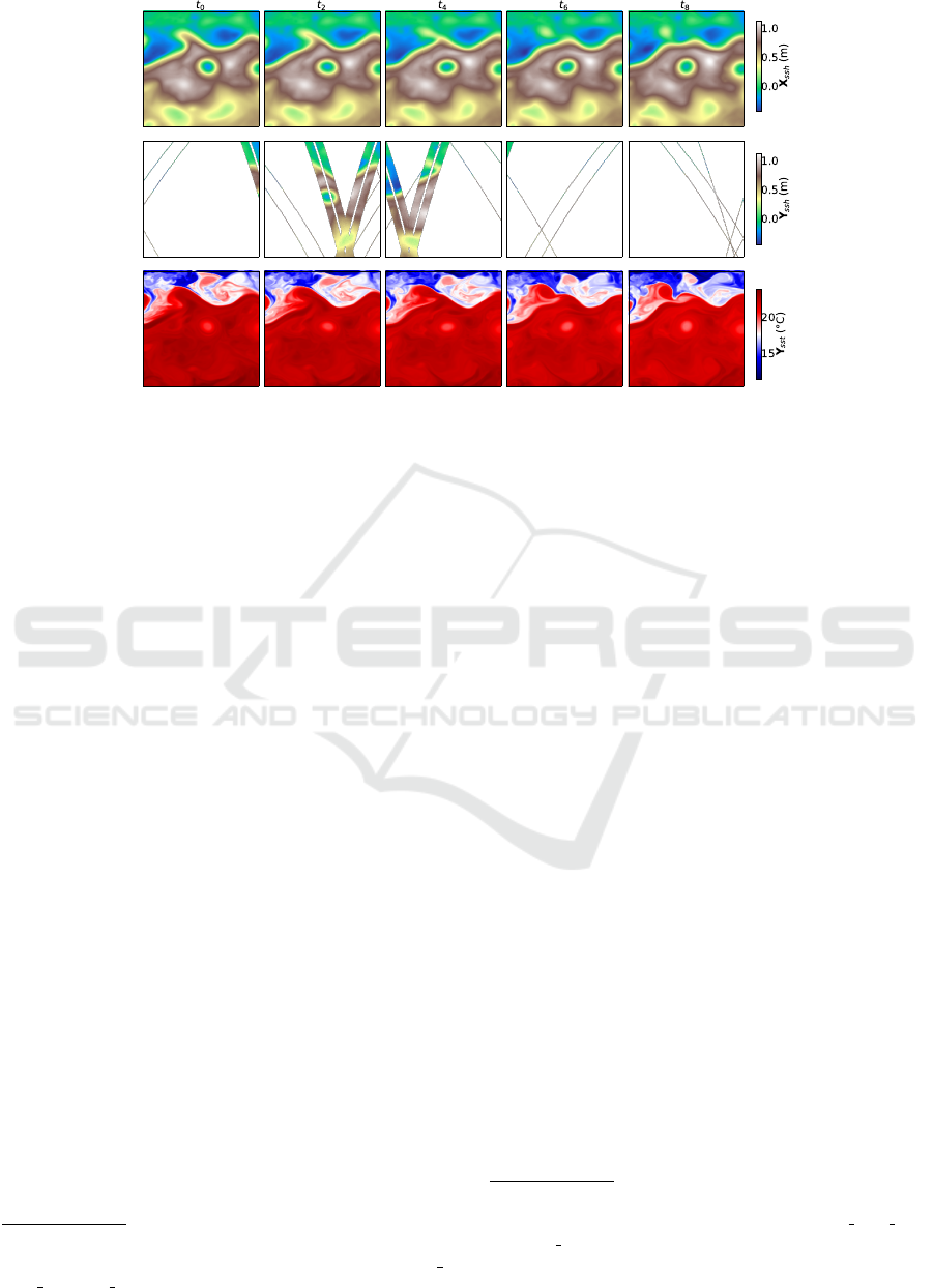
Figure 1: NATL60 output data in a 10-day time window (the time step is 2-day). The ﬁrst row is the ground truth SSH, and

the second is the twin experiment on SSH along tracks. The wide satellite tracks simulate SWOT satellites whereas the ﬁne

tracks simulate nadir observations. The last row is the modeled SST.

2.2.2 Supervised Machine Learning

Machine learning methods, for their part, use statisti-

cal information to learn the inversion. Deep learning

networks can model complex relationships between

multimodal data (Ngiam et al., 2011) and their ﬂex-

ibility makes them suitable to include SST informa-

tion in the interpolation (Nardelli et al., 2022; Ar-

chambault et al., 2022; Fablet et al., 2022). Recently,

(Fablet et al., 2021) introduced 4DVarNet, a super-

vised deep learning network with state-of-the-art per-

formances on simulated data. This method is ﬁtted on

a twin experiment and then applied to the real world.

2.2.3 Unsupervised Machine Learning

Despite supervised schemes, neural network architec-

tures can be used to introduce an inductive bias suited

to image inverse problems as in the paper Deep Image

Prior (DIP) (Ulyanov et al., 2017). Replacing DUACS

BLUE covariance statistics with a Spatio-Temporal

deep image prior is already proven efﬁcient to per-

form the OI of satellite tracks (Filoche et al., 2022).

As they do not need to be trained on full ﬁelds, these

methods can be applied directly to real data.

2.3 Data

In the following, we present two datasets used to

test interpolation methods, the NATL60 Observing

System Simulation Experiment (OSSE)

, and a real-

More information about the OSSE data is pro-

vided at https://github.com/ocean-data-challenges/2020a

SSH mapping NATL60

world scenario with satellite altimetry along tracks

SSH

and SST

2.3.1 Observing System Simulation Experiment

(OSSE)

To test the reconstruction quality of the different

methods we use an Observing System Simulation

Experiment. To do so, a high-resolution simulation

NATL60 (Ajayi et al., 2019) is considered as ground

truth, upon which we simulate satellite orbits and

measurements with realistic instrumental noise. It in-

cludes SWOT wide swaths, and nadir pointing obser-

vations as shown in Figure 1. Both tracks and mea-

surement errors are performed by the swot-simulator

software (Gaultier et al., 2016). As shown in Figure 2,

the daily data coverage of the observations is about

10% on average with strong periodic variations due to

the SWOT satellite’s path. Even when the data cov-

erage reaches 20%, important Spatio-Temporal gaps

remain (see the second row of Figure 1), hence the

difﬁculty of the interpolation task.

To complete the operational framework we use the

SST from NATL60 simulation without noise. This

data is thus not a realistic image as clouds and other

noise sources should be added to be closer to real tem-

perature observations. However, as we will test our

method on real-world data as well, in this ﬁrst experi-

ence we choose not to add any noise to the SST image.

Real-world altimetry data are provided at

https://github.com/ocean-data-challenges/2021a SSH

mapping OSE

MUR SST data are freely available at https://podaac.

jpl.nasa.gov/dataset/MUR-JPL-L4-GLOB-v4.1

Multimodal Unsupervised Spatio-Temporal Interpolation of Satellite Ocean Altimetry Maps

161

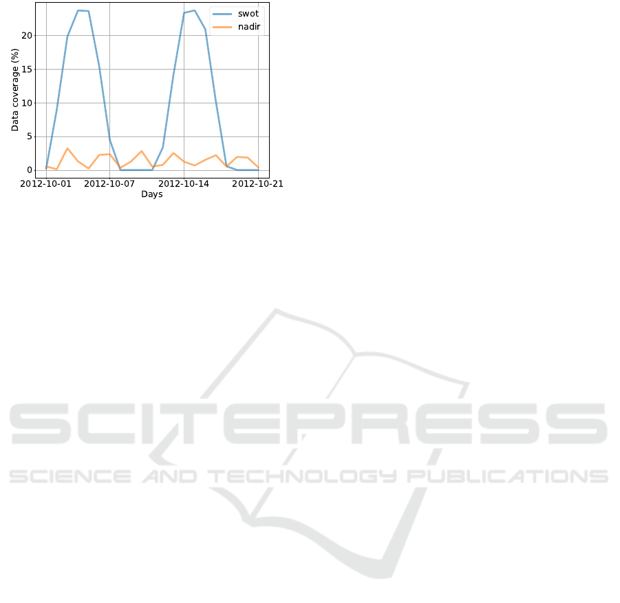
Figure 2: Data coverage on October 2012 with the swot-

simulator software on the study area. The SWOT satellite

provides more points than the multiple nadir satellites but

has a high return time (11 days). Combined, the SWOT and

nadir altimeters cover each day 10.5% of the studied area

on average.

Since this high-resolution simulation is very compu-

tationally intensive, we only have access to one year

of simulation, from the 1

of October 2012 to the 30

of September 2013. The ﬁrst 21 days are used to spin

up the methods that need it, then 42 days of simu-

lation are used as a test set. To avoid data leakage

between the test and the training data, we set aside 31

intermediary days of simulation and take the rest as a

training set.

We focus on a part of the North Atlantic Ocean:

the Gulf Stream area, from latitude 33° to 43° and

from longitude -65° to -55°. This area is very ener-

getic, with strong currents, so we expect a signiﬁcant

synergy between SSH and SST. Also for computa-

tional purposes, we re-grid all images at a resolution

of 0.05° in latitude and longitude (where the NATL60

simulation has a resolution of 0.01°).

2.3.2 Real-World Data

The OSSE data provide an idealistic scenario, with

an optimal combination of altimeters and a noiseless

sea surface temperature. Thus the surface temperature

and height are overly correlated compared to a real-

istic scenario and the multimodal link between data

should be easy to learn by a neural network. This mo-

tivates us to test the same method on real-world data.

We use measures from different nadir altimeters ac-

quired between the 1

of December 2017 to the 31

of January 2018. Once again to evaluate the method

we leave aside the altimeter data from Cryosat-2 as a

test set and some observations of another satellite (Ja-

son 2) as a validation set. We underline the fact that as

the SWOT mission is not launched yet, no data with

wide swaths is available today.

We use temperature data from the Multi-scale

Ultra-high Resolution (MUR) SST (Chin et al., 2017).

These SST satellite images are an operational delayed

time product available with only a 4-day latency.

3 PROPOSED METHOD

3.1 From Supervised to Unsupervised

Inversion

Data assimilation and machine learning methods

leverage different ways to constrain the inversion with

different drawbacks. For instance, the models needed

by data assimilation methods can be computationally

intensive and suffer from various sources of error due

to discretization or unresolved physics among oth-

ers (Janji

c et al., 2018). Also, some of the assim-

ilation methods require the adjoint model which is

not always available. On the other hand, the super-

vised machine learning frameworks need ground truth

and thus use output data of complex physical mod-

els. If 4DVarNet has proven its capacity to interpolate

the simulated data, transposing this training to real-

world scenarios is still challenging and leads to do-

main adaptation issues. The performance of this ap-

proach does not only rely on the ability of a neural

network to learn the physics embedded in the model

but also on the trust that we have in the NATL60 sim-

ulation itself.

Taking into account these elements, we propose a

method, named MUSTI, to train a deep learning net-

work in an operational scenario without using simu-

lations. To that end, we rely on two main features; the

prior induced by the neural network and the statisti-

cal link between the multimodal observations. Our

method differs from 4DVarNet for it is not supervised

on ground truth and from Deep Image Prior as it can

include multimodal observations and is ﬁtted on a

dataset.

3.2 Multimodal Unsupervised

Spatio-Temporal Interpolation

As suggested by the manifold hypothesis (Fefferman

et al., 2016), physical data can be seen as high-

dimension observations taken from the same under-

lying representation. This means that the ocean sys-

tem can be parsimoniously described using a low-

dimension representation vector denoted Z able to en-

code its core dynamics.

Considering the above arguments, using an

encoder-decoder framework seems appropriate. One

VISAPP 2023 - 18th International Conference on Computer Vision Theory and Applications

162

Figure 3: Computation graph of the proposed method. The neural network h

holds all the control parameters θ and aims to

generate a time series of SSH images from a time series of SST images. This method can use any kind of neural network

architecture for h

, as long as it takes an image time series as input and output. The masking operator H

Ω

is applied before

the cost function in order to train the network in an unsupervised manner.

can use a deep neural network to encode Y

sst

in the

latent space by modeling p(Z|Y

sst

). A decoder can

then recover the output distribution p



ssh



and

transfer information from the SST gridded image to a

SSH image. Hereafter the encoder will be denoted f

in Eq. (3), the decoder g

in Eq. (4) and the encoder-

decoder network h

= g

◦ f

. Other architectures

can be used as well through a direct multimodal in-

formation transfer from Y

sst

to X

ssh

as long as they

bring an inductive bias, helping the reconstruction.

Encoding:

Z = f

sst

) (3)

Decoding:

ssh

= g





(4)

Masking:

ssh

= H

Ω



ssh



(5)

The MUSTI method consists in encoding the SST

observations as in Eq. (3) as a latent vector

Z. Then

following Eq. (4) the SSH gridded state

ssh

is esti-

mated from the latent space. Finally, as we want the

neural network to be trained in an unsupervised way,

we apply the masking operator H

Ω

to the estimate

SSH state

ssh

to retrieve along-tracks observations

ssh

as Eq. (4) suggests.

By doing so, we can supervise the network only

on the pixels where we have access to observations.

This means that, similarly to Deep Image Prior in-

painting scheme (Ulyanov et al., 2017), we compute

a supervised loss L between

ssh

and Y

ssh

, Eq. (6).



ssh

, Y

ssh



∑

t=0



ssh

−Y

ssh



∑

t=0



Ω



ssh



−Y

ssh



(6)

The MUSTI method aims in learning a multi-

modal physical link between the gridded SST and the

along-track SSH. The implicit hypothesis behind our

method is that ﬁtting a neural architecture to model



ssh

sst



will provide a good estimation of the

true state X

ssh

even on the pixels where it is not super-

vised to do so. We believe that due to the symmetry

by translation of the convolution operation, the fea-

tures learned on along tracks measurements will ap-

ply the same physical transformation to every pixel of

the SST image to generate the gridded SSH map. We

present a visual overview of this method in Figure 3.

4 RESULTS

4.1 Experiment

The MUSTI training procedure can be used with

a wide range of convolutional neural architectures

as long they bring an inductive bias toward out of

tracks generalization. We test two deep neural net-

work architectures following the MUSTI method: a

U-net architecture (Ronneberger et al., 2015) and a

Spatio-Temporal auto-encoder (STAE). It relies on

the Spatio-Temporal convolution (conv2DP1) intro-

duced by (Tran et al., 2018). More details about

the STAE architecture are provided in Appendix B.

Previous work has shown that this kind of convolu-

tion introduces a Spatio-Temporal prior well suited

for satellite track interpolation in an unlearned frame-

work (Filoche et al., 2022). Using a network architec-

ture relying on the same principles, we use conv2DP1

and 3D maxpooling to reduce the time series spatial

dimension while preserving time encoding.

Thus we can compare the performance of a net-

work compressing information in a latent space and

the performance of a direct network. Hereafter we

will discuss 3 different scenarios: the OSSE data with

Multimodal Unsupervised Spatio-Temporal Interpolation of Satellite Ocean Altimetry Maps

163

Table 1: Results of the different methods on the three data scenarios. We present hereafter the score of the different interpola-

tion methods to which we compare ourselves. We give the score of the MUSTI method for an ensemble of 10 neural networks

with different weights initialization and the mean performance of each member of the ensemble. The details about the tuned

hyper-parameters are given in Appendix A

swot + nadir nadir only real-world data

Methods µ σ

µ σ

DUACS 0.922 0.017 1.22 11.29 0.916 0.008 1.42 12.08 0.877 0.065

DYMOST 0.926 0.018 1.19 10.26 0.911 0.013 1.35 11.87 0.889 0.064

MIOST 0.938 0.012 1.18 10.33 0.927 0.007 1.34 10.34 0.887 0.085

BFN 0.926 0.018 1.02 10.37 0.919 0.017 1.23 10.64 0.879 0.065

4DVarNet

∗

0.959 0.009 0.62 4.31 0.944 0.006 0.84 7.95 0.889 0.089

MUSTI U-net mean 0.951 0.01 1.09 6.0 0.939 0.009 1.35 5.73 0.881 0.103

MUSTI U-net ensemble 0.954 0.009 0.62 3.44 0.946 0.008 1.23 4.14 0.886 0.099

MUSTI STAE mean 0.945 0.011 1.02 6.32 0.931 0.012 1.13 8.78 0.885 0.086

MUSTI STAE ensemble 0.952 0.011 0.68 5.41 0.938 0.012 0.96 7.59 0.893 0.083

∗

supervised

SWOT and nadir measures, with only nadir measures,

and the real-world data.

4.1.1 Training Procedure

For each scenario and neural architecture we tune the

window size T , and the stopping epoch on the val-

idation dataset, as described in Appendix C. FLAG

In the real-world scenario, there is no ground truth to

serve as a validation dataset, therefore we leave aside

the observations from a satellite (Jason-2g) to tune

the model’s hyper-parameters on. Once these hyper-

parameters are found on validation observations, we

train another network with this set of parameters on

the training and validation set. This way we can fully

compare to other methods in terms of used altimetry

observations.

As the optimization path varies with weight ini-

tialization, we train a set of 10 models for each experi-

ence and average generated images from each model.

This ensemble of neural networks helps to stabilize

performances regarding to initialization and is proven

to enhance the reconstruction (Filoche et al., 2022;

Hinton and Dean, 2015).

4.1.2 Method Evaluation

To compare the reconstruction methods we use the

metrics deﬁned by (Le Guillou et al., 2020) includ-

ing the normalized root mean squared (NRMSE) as in

Eq. (7):

NRMS E (t, y,

y) = 1 −

RMSE (y

)

RMS (y)

(7)

with Root Mean Squared Error as RMSE and with

Root Mean Squared of the target y during the entire

evaluation time domain as RMS (y). We call in Ta-

ble 1 µ the mean of the NRMSE on the time domain

and σ

its time standard deviation. These metrics have

no units and for a perfect reconstruction µ equals 1.

We also use two spectral metrics, λ

(in degrees)

and λ

(in days) that can be assimilated respectively

to the minimum spatial and temporal wavelength re-

solved. We do not compute these spectral metrics

for the real-world scenario, because we do not have

a gridded ground truth. For more details about the

implementation of these metrics, we refer the reader

to (Le Guillou et al., 2020). All metrics given in Ta-

ble 1 are computed on the image at the center of the

time series.

4.2 Comparison of the Methods on

OSSE and Real-World Data

We compare the results of different methods: the op-

erational linear interpolation using a covariance ma-

trix tuned with 25 years of observations (DUACS),

three model-based data assimilation schemes: DY-

MOST (Ubelmann et al., 2016; Ballarotta et al., 2020),

MIOST (Ardhuin et al., 2020) and BFN (Le Guillou

et al., 2020). Finally, we compare with the supervised

neural network 4DVarNet (Fablet et al., 2021).

• In the swot + nadir scenario 4DVarNet outper-

forms other methods in terms of RMSE, espe-

cially DUACS and the model-driven approaches.

The MUSTI method can not compare with the su-

pervised scheme RMSE-wise but has similar re-

sults in terms of minimum spatial and tempo-

ral wavelength resolved. The U-net architecture

gives better results than STAE. In Figure 4 we

present a visual comparison of the DUACS method

and a MUSTI U-net. We see that the DUACS

method misses some of the small-scale variations

that the MUSTI method is able to resolve.

VISAPP 2023 - 18th International Conference on Computer Vision Theory and Applications

164

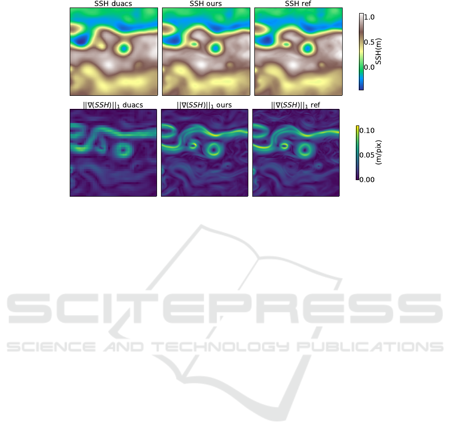
Figure 4: Visual overview of the visual results in the swot+nadir scenario. We compare DUACS and an U-net trained

following the MUSTI method. We present the generated SSH image and the norm of the gradient.

• In the nadir only scenario, no wide swath altime-

try data are available, thus the performances of

all unsupervised methods drop by approximately

0.01 in terms of normalized RMSE. But the su-

pervised neural network has a higher performance

drop, so in the end, the U-net trained in a MUSTI

way has a slightly better RMSE and temporal res-

olution. However, we notice a signiﬁcant drop in

the reconstruction of the short spatial wavelength.

This can be explained by the fact that lacking large

satellite swath, the small eddies are missed.

• On the real-world data, every method has a

very signiﬁcant RMSE performance drop. The

DYMOST, MIOST, and 4DVarNet methods are in

a nutshell, while DUACS and BFN are outper-

formed. Surprisingly, the two networks trained

with MUSTI method do not have the same order

of performance as on the OSSE data. The STAE

ensemble outperforms other methods, while the

U-net does not reach DYMOST, MIOST and

4DVarNet. It seems that the encoding-decoding

process is useful to denoise the SST images while

a skip connection is not able to do so.

These results demonstrate the potential of un-

supervised neural networks to deal with partially

observed ﬁelds. The MUSTI method that was designed

for an operational framework achieves better results

in the real-world scenario, directly learning from real-

world ﬁelds than a method supervised on an indepen-

dent dataset. Furthermore, we show that it is possible

to transfer multimodal information from the SST to

the SSH ﬁelds without providing any covariance ma-

trix, physical model information, or supervision

with a full-ﬁeld dataset.

5 PERSPECTIVES

In the following, we discuss different ways to con-

tinue this work.

Using MUSTI Method in a Transfer Learning

Scheme. Our method allows us to train a neural net-

work with incomplete data as an operational frame-

work requires. However, this method could also be

used in a transfer learning scheme. We are interested

in training a deep learning architecture on OSSE data

in a traditional supervised way, and then using MUSTI

method to ﬁne-tune the model on real-world data.

Multimodal Fusion. There are different ways to

perform multimodal data fusion (Ngiam et al., 2011)

and we are interested in testing other fusion ap-

proaches. For instance, if this training procedure is

capable to ﬁt a trajectory of SST to a trajectory of

SSH it does not generalize well to new examples. Be-

ing able to give SSH ground tracks as inputs of the

network without overﬁtting them should help solve

this problem.

6 CONCLUSION

We presented a method to include multimodal infor-

mation in Spatio-Temporal image inverse problems in

Multimodal Unsupervised Spatio-Temporal Interpolation of Satellite Ocean Altimetry Maps

165

an unsupervised way. Relying on the hidden physi-

cal link between Sea Surface Height and Sea Surface

Temperature, we train a neural network to ﬁt the SSH

along tracks observations starting from a fully grid-

ded SST image. We show that the multimodal trans-

fer performed by the network on the along-tracks data

generalizes well where it has not been supervised. We

tested two different neural architectures, a U-net and

a Spatio-Temporal auto-encoder, on 3 datasets (2 sim-

ulations and a real-world scenario).

On real-world data, we report a relative improve-

ment of 13% compared to the operational product

(DUACS) in terms of RMSE. We also show that

our method is able to outperform supervised state-

of-the-art interpolation architectures as they suffer

from overﬁtting of the simulation upon which they are

trained.

REFERENCES

Ajayi, A., Le Sommer, J., Chassignet, E., Molines, J.-M.,

Xu, X., Albert, A., and Cosme, E. (2019). Spatial

and temporal variability of north atlantic eddy ﬁeld at

scale less than 100 km. Earth and Space Science Open

Archive, page 28.

Amores, A., Jord

a, G., Arsouze, T., and Le Sommer, J.

(2018). Up to what extent can we characterize ocean

eddies using present-day gridded altimetric products?

Journal of Geophysical Research: Oceans, 123:7220–

7236.

Archambault, T., Charantonnis, A., B

eziat, D., and Thiria,

S. (2022). SSH Super-Resolution using high resolu-

tion SST with a Subpixel Convolutional Residual Net-

work. In Climate Informatics.

Ardhuin, F., Ubelmann, C., Dibarboure, G., Gaultier, L.,

Ponte, A., Ballarotta, M., and Faug

ere, Y. (2020). Re-

constructing ocean surface current combining altime-

try and future spaceborne doppler data. Earth and

Space Science Open Archive.

Ballarotta, M., Ubelmann, C., Rog

e, M., Fournier, F.,

Faug

ere, Y., Dibarboure, G., Morrow, R., and Picot,

N. (2020). Dynamic mapping of along-track ocean al-

timetry: Performance from real observations. Journal

of Atmospheric and Oceanic Technology, 37:1593–

1601.

Bretherton, F., Davis, R., and Fandry, C. (1976). A tech-

nique for objective analysis and design of oceano-

graphic experiments applied to MODE-73. Deep-Sea

Research and Oceanographic Abstracts, 23:559–582.

Chin, T. M., Vazquez-Cuervo, J., and Armstrong, E. M.

(2017). A multi-scale high-resolution analysis of

global sea surface temperature. Remote Sensing of En-

vironment, 200:154–169.

Ciani, D., Rio, M.-H., Bruno Nardelli, B., Etienne, H., and

Santoleri, R. (2020). Improving the altimeter-derived

surface currents using sea surface temperature (SST)

data: A sensitivity study to SST products. Remote

Sensing, 12:1601.

Emery, W. J., Brown, J., and Nowak, Z. P. (1989). AVHRR

image navigation-summary and review. Photogram-

metric engineering and remote sensing, 4:1175–1183.

Fablet, R., Amar, M., Febvre, Q., Beauchamp, M., and

Chapron, B. (2021). End-to-end physics-informed

representation learning for satellite ocean remote

sensing data: Applications to satellite altimetry and

sea surface currents. ISPRS Annals of the Photogram-

metry, Remote Sensing and Spatial Information Sci-

ences, 5:295–302.

Fablet, R., Febvre, Q., and Chapron, B. (2022). Multimodal

4DVarNets for the reconstruction of sea surface dy-

namics from sst-ssh synergies. ArXiv.

Fefferman, C., Mitter, S., and Narayanan, H. (2016). Test-

ing the manifold hypothesis. Journal of the American

Mathematical Society, 29:983–1049.

Filoche, A., Archambault, T., Charantonis, A., and

eziat, D. (2022). Statistics-free interpolation of

ocean observations with deep spatio-temporal prior.

In ECML/PKDD Workshop on Machine Learning for

Earth Observation and Prediction (MACLEAN).

Gaultier, L., Ubelmann, C., and Fu, L. (2016). The chal-

lenge of using future SWOT data for oceanic ﬁeld

reconstruction. Journal of Atmospheric and Oceanic

Technology, 33:119–126.

Hinton, G. and Dean, J. (2015). Distilling the knowledge in

a neural network. In NIPS Deep Learning and Repre-

sentation Learning Workshop.

Jam, J., Kendrick, C., Walker, K., Drouard, V., Hsu, J., and

Yap, M. (2021). A comprehensive review of past and

present image inpainting methods. Computer Vision

and Image Understanding, 203.

Janji

c, T., Bormann, N., Bocquet, M., Carton, J. A., Cohn,

S. E., Dance, S. L., Losa, S. N., Nichols, N. K., Pot-

thast, R., Waller, J. A., and Weston, P. (2018). On

the representation error in data assimilation. Quar-

terly Journal of the Royal Meteorological Society,

144(713):1257–1278.

Klein, P., Isem-Fontanet, J., Lapeyre, G., Roullet, G., Dan-

ioux, E., Chapron, B., Le Gentil, S., and Sasaki, H.

(2009). Diagnosis of vertical velocities in the upper

ocean from high resolution sea surface height. Geo-

physical Research Letters, 36.

Le Guillou, F., Metref, S., Cosme, E., Ubelmann, C., Bal-

larotta, M., Verron, J., and Le Sommer, J. (2020).

Mapping altimetry in the forthcoming SWOT era by

back-and-forth nudging a one-layer quasi-geostrophic

model. Earth and Space Science Open Archive.

Leuliette, E. W. and Wahr, J. M. (1999). Coupled

pattern analysis of sea surface temperature and

TOPEX/Poseidon sea surface height. Journal of Phys-

ical Oceanography, 29(4):599–611.

McCann, M., Jin, K., and Unser, M. (2017). Convolutional

neural networks for inverse problems in imaging: A

review. IEEE Signal Processing Magazine, 34:85–95.

Nardelli, B., Cavaliere, D., Charles, E., and Ciani, D.

(2022). Super-resolving ocean dynamics from space

VISAPP 2023 - 18th International Conference on Computer Vision Theory and Applications

166

with computer vision algorithms. Remote Sensing,

14:1159.

Ngiam, J., Khosla, A., Kim, M., Nam, J., Lee, H., and Ng,

A. Y. (2011). Multimodal deep learning. In Proceed-

ings of the 28th International Conference on Interna-

tional Conference on Machine Learning, ICML 11,

page 689–696, Madison, WI, USA. Omnipress.

Ongie, O., Jalal, A., Metzler, C., Baraniuk, R., Dimakis,

A., and Willett, R. (2020). Deep learning techniques

for inverse problems in imaging. IEEE Journal on

Selected Areas in Information Theory, 1:39–56.

Qin, Z., Zeng, Q., Zong, Y., and Xu, F. (2021). Image in-

painting based on deep learning: A review. Displays,

69:102028.

Ronneberger, O., Fischer, P., and Brox, T. (2015). U-net:

Convolutional networks for biomedical image seg-

mentation. In MICAI, pages 234–24.

Stegner, A., Le Vu, B., Dumas, F., Ghannami, M., Nicolle,

A., Durand, C., and Faugere, Y. (2021). Cyclone-

anticyclone asymmetry of eddy detection on gridded

altimetry product in the mediterranean sea. Journal of

Geophysical Research: Oceans, 126.

Taburet, G., Sanchez-Roman, A., Ballarotta, M., Pujol, M.-

I., Legeais, J.-F., Fournier, F., Faugere, Y., and Dibar-

boure, G. (2019). DUACS DT2018: 25 years of re-

processed sea level altimetry products. Ocean Sci,

15:1207–1224.

Tran, D., Wang, H., Torresani, L., Ray, J., Lecun, Y., and

Paluri, M. (2018). A closer look at spatiotemporal

convolutions for action recognition. Proceedings of

the IEEE Computer Society Conference on Computer

Vision and Pattern Recognition, pages 6450–6459.

Ubelmann, C., Cornuelle, B., and Fu, L. (2016). Dynamic

mapping of along-track ocean altimetry: Method and

performance from observing system simulation exper-

iments. Journal of Atmospheric and Oceanic Technol-

ogy, 33:1691–1699.

Ulyanov, D., Vedaldi, A., and Lempitsky, V. (2017). Deep

image prior. International Journal of Computer Vi-

sion, 128:1867–1888.

Wang, Z., Chen, J., and Hoi, S. (2021). Deep learning for

image super-resolution: A survey. IEEE Transactions

on Pattern Analysis and Machine Intelligence, pages

3365–3387.

A Implementation Details

All networks are trained through an ADAM optimizer

with the following parameters: β

= 0.9, β

= 0.999.

We use an exponential learning rate scheduler with

a starting learning rate of 10

−3

for the U-net and of

5 × 10

−4

for the STAE and α = 0.96.

We determine the optimal hyper-parameters (win-

dow temporal size T and stopping epoch) on the vali-

dation dataset, other hyper-parameters are untuned.

Table 2: Optimal hyper-parameters on the validation dataset

for each architecture and dataset.

Dataset STAE U-net

T epoch T epoch

s+n 7 94 3 113

n 5 57 5 60

rw 5 50 5 55

B Network Architectures

Spatio-Temporal Auto-Encoder

The architecture of the Spatio-Temporal Auto-

Encoder (STAE) is given in our code and relies on the

Conv2PD1 introduced by (Tran et al., 2018). First,

a 2D convolution is performed in the spatial dimen-

sions, then a 3D Batch-Normalization followed by a

ReLU activation function and ﬁnally a 1D convolu-

tion in the time dimension. The spatial dimensions of

the image are then divided by 2 (the time dimension

is not reduced) with a 3D max pooling.

The decoder is similar to the encoder except

that we use a 3D upsampling (trilinear) and then

a Conv2DP1. The last block has no Batch-

Normalization nor ReLU activation function.

U-net

The U-net (Ronneberger et al., 2015) architecture is

a classic image architecture. We use four downward

blocks composed of two 2D convolutions, each one

with a ReLU activation function and BatchNormal-

ization. A Maxpooling is then performed to divide

the size of the image by two.

C Train, Validation, Test Split

Table 3: Train, validation, and test datasets for each sce-

nario

Dataset OSSE Real-world

Train Tracks from all

year

every nadir

satellite except

j2g and c2

Validation GT between

2013-01-02 and

2013-09-30

nadir tracks

from j2g

satellite

Test GT between

2012-10-22 and

2012-12-02

nadir tracks

from c2 satellite

our code is available at https://gitlab.lip6.fr/

archambault/visapp2023

Multimodal Unsupervised Spatio-Temporal Interpolation of Satellite Ocean Altimetry Maps

167