Hybrid Methods to Solve the Two-Stage Robust Flexible Job-Shop

Scheduling Problem with Budgeted Uncertainty

Carla Juvin

, Laurent Houssin

1,2 a

and Pierre Lopez

1 b

LAAS-CNRS, Universit

e de Toulouse, CNRS, Toulouse, France

ISAE-SUPAERO, Toulouse, France

Keywords:

Flexible Job-Shop Scheduling, Robust Optimization, Uncertainty Budget, Mixed Integer Linear

Programming, Constraint Programming.

Abstract:

This paper addresses the robust ﬂexible job-shop scheduling problem considering uncertain operation pro-

cessing times associated with an uncertainty budget. Exact solution methods based on mixed integer linear

programming and constraint programming are proposed to solve the problem. Such solutions are hybridized in

the framework of a two-stage robust optimization, and a column and constraint generation algorithm is used to

solve representative instances. The experimental results show the advantages of a two-stage approach where

constraint programming and integer programming are mixed to solve a master problem and a subproblem,

respectively.

1 INTRODUCTION

The job-shop scheduling problem is a well studied

and NP-hard problem where a set of jobs are to be

processed on a set of machines (Garey et al., 1976).

Each job is composed of a sequence of operations that

must be processed on machines with given processing

times in a given job-dependent order, and each ma-

chine can process only one operation at a time. The

ﬂexible job-shop problem (FJSSP) is a generalization

of the job-shop scheduling problem: for each oper-

ation, there exists a set of eligible machines. This

makes the problem more difﬁcult to solve, as it con-

sists of both a machine allocation and a sequencing

problem. The FJSSP has received considerable atten-

tion and both metaheuristics and exact methods have

been developed to solve the problem, the majority of

them with the assumption that the parameters are de-

terministically known (Brandimarte, 1993; Dauz

ere-

es and Paulli, 1997). However, in the real world,

many sources of uncertainty (processing times varia-

tion, machine breakdown, addition of new operations,

etc.) can affect the quality and even the feasibility of

a schedule.

There exist two major approaches to deal with

data uncertainty: stochastic optimization and robust

https://orcid.org/0000-0001-5975-7639

https://orcid.org/0000-0003-0413-3188

optimization. While stochastic optimization consid-

ers probability distribution, robust optimization as-

sumes that uncertain data belong to a given uncer-

tainty set and aims to optimize performance consid-

ering the worst-case scenario within that set.

In this paper, we propose exact solution meth-

ods to solve the robust ﬂexible job-shop scheduling

problem. A two-stage robust optimization is used to

deal with processing times uncertainty, where the ﬁrst

stage ﬁxes the assignment and the sequence of opera-

tions on machines whilst the second stage sets the op-

eration start times. We provide two robust counterpart

models based on mixed-integer linear programming

and constraint programming formulations, as well as

a column and constraint generation algorithm. A dis-

cussion is conducted on the basis of an analysis of

experimental results.

2 PROBLEM DEFINITION

2.1 Deterministic Flexible Job-Shop

Scheduling Problem

We ﬁrst introduce the ﬂexible job-shop scheduling

problem (FJSSP) with makespan minimization. An

instance of the FJSSP implies a set of jobs J and a set

of machines M . Each job i ∈ J consists of a sequence

Juvin, C., Houssin, L. and Lopez, P.

Hybrid Methods to Solve the Two-Stage Robust Flexible Job-Shop Scheduling Problem with Budgeted Uncertainty.

DOI: 10.5220/0011619700003396

In Proceedings of the 12th International Conference on Operations Research and Enterprise Systems (ICORES 2023), pages 135-142

ISBN: 978-989-758-627-9; ISSN: 2184-4372

 2023 by SCITEPRESS – Science and Technology Publications, Lda. Under CC license (CC BY-NC-ND 4.0)

135

of n

operations. The j

operation O

i, j

∈ O

of a job

i must be performed by one of the machines from the

set of eligible machines M

i, j

⊆ M . Let p

i, j,m

denote

the processing time of operation O

i, j

that is processed

on machine m ∈ M

i, j

. Each machine can process at

most one operation at a time and preemption is not

allowed: once an operation is started, it must be pro-

cessed without any interruption. The objective is to

ﬁnd an assignment for each operation and a sequence

on each machine that minimize the maximum com-

pletion time or makespan C

max

Notations and Deﬁnitions.

J Set of jobs

M Set of machines

Number of operations in job i (i ∈ J )

Set of operations in job i (i ∈ J )

i, j

operation of job i (i ∈ J , j ∈ {1, . . . , n

})

i, j

Set of eligible machines for operation

i, j

(i ∈ J , O

i, j

∈ O

)

i, j,m

Processing time of operation O

i, j

machine m (i ∈ J , O

i, j

∈ O

, m ∈ M

i, j

)

Set of operations that can be processed by

machine m (m ∈ M )

H Big constant

2.2 Flexible Job-Shop Scheduling

Problem with Uncertain Processing

Times

We consider that the processing times of operations

are uncertain. Each processing time p

i, j,m

of an oper-

ation O

i, j

∈ O

, i ∈ J , on machine m ∈ M

i, j

, belongs to

the interval [ ¯p

i, j,m

, ¯p

i, j,m

+ ˆp

i, j,m

], where ¯p

i, j,m

is the

nominal value and ˆp

i, j,m

the maximum deviation of

the processing time from its nominal value.

Example 1. Consider an FJSSP instance with 3 jobs

and 2 machines. The intervals [ ¯p

i, j,m

, ¯p

i, j,m

+ ˆp

i, j,m

]

of processing times p

i, j,m

of operations O

i, j

∈ O

, i ∈

J on each eligible machine m ∈ M

i, j

, are given in Ta-

ble 1.

Table 1: Numerical example of an instance of the FJSSP:

operation processing times.

M1 M2

1,1

[43; 86] –

J1 O

1,2

[87; 170] [95; 190]

2,1

[63; 142] [53; 166]

J2 O

2,2

– [73; 131]

3,1

[125; 239] [135; 224]

J3 O

3,2

[43; 73] [61; 174]

2.2.1 Uncertainty Budget

The traditional robust optimization approach (Soys-

ter, 1973) consists in protecting against the case when

all parameters can deviate at the same time, which

makes the solution overly conservative. Indeed, there

is a very low probability that all parameters take their

worst value all together. To overcome this limitation,

(Bertsimas and Sim, 2004) introduce an uncertainty

budget approach that allows a restriction on the num-

ber of deviations that can occur simultaneously to a

given budget. In order to reach a trade-off between

robustness and solution quality, we exploit this ap-

proach to deﬁne the uncertainty set.

Let Γ be the budget of uncertainty, the maximum

number of operations whose processing time devia-

tion can occur simultaneously. The worst-case sce-

nario is always an extremum scenario (Ben-Tal et al.,

2009). Thus, for each scenario ξ, the processing time

of operation O

i, j

on machine m is given by:

i, j,m

(ξ) = ¯p

i, j,m

+ ξ

i, j

· ˆp

i, j,m

where ξ

i, j

is equal to 1 if the processing time of the

operation deviates, 0 otherwise.

We deﬁne the uncertainty set U

as:

= {(ξ

i, j

)

i∈J ,1≤ j≤n

∑

i∈J

∑

j=1

i, j

≤ Γ}

2.2.2 Multi-Stage Robust Optimization

Multi-stage robust optimization has been introduced

by (Ben-Tal et al., 2004). In some optimization prob-

lems, only part of the decision variables have to be

ﬁxed before uncertainty is revealed, while the other

variables can be chosen after the realization and can

thus be adjusted to the scenario. The authors intro-

duce the adjustable robust counterpart; the set of de-

cision variables is split into “here and now” decisions

and “wait and see” decisions. The objective is to ﬁnd

a solution for the “here and now” decision variables

such that constraints involving uncertain parameters

remain feasible for all values of the uncertain param-

eters, and minimizing the objective value.

In our problem, we consider that the purpose is

to ﬁnd the assignment and sequence on the machines

(ﬁrst stage: here and now), allowing to deﬁne a start

time for each operation and each scenario (second

stage: wait and see), minimizing the makespan in the

worst-case scenario considering the budget of uncer-

tainty.

Example 2. Considering Example 1, a feasible solu-

tion is the assignment of operations O

1,1

, O

3,1

, O

3,2

machine M

, and of operations O

2,1

, O

2,2

, O

1,2

to ma-

chine M

, following these sequences. Figure 1 repre-

sents this solution when all processing times take their

ICORES 2023 - 12th International Conference on Operations Research and Enterprise Systems

136

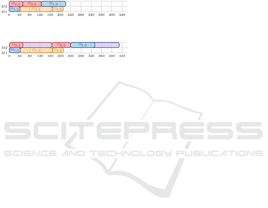
nominal value; the makespan is 221. Considering an

uncertainty budget Γ = 2, the worst case, for this so-

lution, is that the processing time of operations O

2,1

and O

1,2

deviate and take their greatest value. Fig-

ure 2 shows the Gantt chart in this case. The objec-

tive function value of this solution for an uncertainty

budget Γ = 2 reaches the makespan equal to 429.

Figure 1: A feasible solution for Example 1, when all pro-

cessing times take their nominal value.

Figure 2: From the solution of Figure 1, the worst-case so-

lution with an uncertainty budget of 2.

3 ROBUST COUNTERPART FOR

THE FJSSP

Two robust counterparts of the ﬂexible job-shop

scheduling problem are presented. They are respec-

tively based on a Mixed Integer Linear Programming

formulation and a Constraint Programming model for

the deterministic FJSSP.

3.1 Mixed Integer Linear Programming

Model

We deﬁne a Mixed Integer Linear Programming

(MILP) extended robust model, which is directly

inspired by the sequence-based model made by (Shen

et al., 2018). The ﬁrst stage decision variables are

deﬁned as follows:

i, j,m







1 if operation O

i, j

is processed on

machine m;

0 otherwise

i, j,i

, j







1 if operation O

i, j

is processed before

, j

;

0 otherwise

while the start time t

i, j

(ξ) ∈ R

of each operation O

i, j

in scenario ξ is part of the second stage variables.

The MILP model is as follows:

minC

max

(1)

s.t.

∑

m∈M

i, j

i, j,m

= 1 ∀i ∈ J ,∀ j ∈ O

(2)

∑

m∈M

i, j−1

i, j−1,m

· p

i, j−1,m

(ξ) +t

i, j−1

(ξ) ≤ t

i, j

(ξ)

∀i ∈ J , ∀ j ∈ O

, ∀ξ ∈ U

(3)

, j

(ξ) + p

, j

(ξ) − (2 − x

i, j,m

− x

, j

+ y

i, j,i

, j

) · H

≤ t

i, j

(ξ) ∀m ∈ M , ∀(O

i, j

, O

i, j

) ∈ I

, ∀ξ ∈ U

(4)

i, j

(ξ) + p

i, j,m

(ξ) − (3 − x

i, j,m

− x

, j

− y

i, j,i

, j

) · H

≤ t

, j

(ξ) ∀m ∈ M , ∀(O

i, j

, O

i, j

) ∈ I

, ∀ξ ∈ U

(5)

i,n

(ξ) +

∑

m∈M

i,n

· p

i,n

(ξ) ≤ C

max

∀i ∈ J , ∀ξ ∈ U

(6)

i, j,m

∈

{

0, 1

}

∀i ∈ J , ∀ j ∈ O

, ∀m ∈ M

i, j

(7)

i, j,i

, j

∈

{

0, 1

}

∀(i, i

) ∈ J

, ∀ j ∈ O

, ∀ j

∈ O

(8)

The objective (1) is to minimize the makespan

max

. Constraints (2) are assignment constraints and

ensure that each operation is assigned to exactly one

machine. Constraints (3) ensure the precedence rela-

tion between two consecutive operations of the same

job. Constraints (4) and (5) are the disjunctive con-

straints and avoid overlapping of operations sched-

uled on the same machine. Note that Constraints (3),

(4) and (5) are duplicated for each feasible scenario.

Finally, Constraints (6) allow to compute the greatest

makespan among all feasible scenarios and therefore

to determine the optimal solution in the worst case.

Finally, Constraints (7) and (8) deﬁne the domain of

the variables.

3.2 Constraint Programming Model

While Constraint Programming (CP) obtains very

good results in scheduling, to the best of our knowl-

edge it has been never used in robust multi-stage mod-

els. The following model is directly inspired from

(Kress and M

uller, 2019) for the deterministic FJSSP

with machine operator constraints. It involves the fol-

lowing variables:

• task

i, j,ξ

: interval variable between the start and

the end of the processing of operation O

i, j

in sce-

nario ξ;

• mode

i, j,m,ξ

: interval variable between the start and

the end of the processing of operation O

i, j

on ma-

chine m in scenario ξ (since the operations have

multiple eligible machines and must be executed

by exactly one of them, this is an optional vari-

able);

• seqs

m,ξ

: sequence variable of tasks scheduled on

machine m in scenario ξ.

Hybrid Methods to Solve the Two-Stage Robust Flexible Job-Shop Scheduling Problem with Budgeted Uncertainty

137

The CP model is as follows:

minC

max

(9)

s.t.

max

≥ task

i,n

,ξ

.end ∀i ∈ J , ∀ξ ∈ U

(10)

EndBe f oreStart(task

i, j,ξ

,task

i, j+1,ξ

)

∀i ∈ J , ∀O

i, j

∈ O

\ {O

i,n

}, ∀ξ ∈ U

(11)

Al ternative(task

i, j,ξ

, mode

i, j,m,ξ

: ∀m ∈ M

i, j

)

∀i ∈ J , ∀O

i, j

∈ O

, ∀ξ ∈ U

(12)

NoOverlap(seqs

m,ξ

) ∀m ∈ M , ∀ξ ∈ U

(13)

PresenceO f (mode

i, j,m,0

) ⇒ PresenceO f (mode

i, j,m,ξ

)

∀i ∈ J , ∀O

i, j

∈ O

, ∀m ∈ M

i, j

, ∀ξ ∈ U

\ {0} (14)

SameSequence(seqs

m,0

, seqs

m,ξ

)

∀m ∈ M , ∀ξ ∈ U

\ {0} (15)

Constraints (10) allow the determination of the

makespan, which is equal to the end of the last op-

eration. Constraints (11) ensure the precedence rela-

tion between two consecutive operations of the same

job. Constraints (12) ensure that each operation is as-

signed to exactly one machine. Constraints (13) en-

sure that in each scenario each machine performs at

most only one operation at the same time. Constraints

(10–13) are duplicated for each scenario. Constraints

(14) and (15) ensure that the assignment of each oper-

ation and the sequence on each machine are the same

in each scenario. For these last two constraints, the

ﬁrst scenario ξ = 0 is used as reference.

4 COLUMN AND CONSTRAINT

GENERATION APPLIED TO

THE FJSSP

We present here a column and constraint genera-

tion approach to solve the robust ﬂexible job-shop

scheduling problem. This method has been intro-

duced by (Zeng and Zhao, 2013) to solve two-stage

robust optimization problems. The procedure splits

the problem into a master problem and an adversarial

subproblem. The idea is to solve the robust counter-

part problem (or master problem), for a limited sub-

set of scenarios, and then to identify which scenarios,

if any, make the found solution infeasible, using an

adversarial subproblem. Then, these scenarios are in-

cluded in the master problem by generating the corre-

sponding recourse decision variables on the ﬂy. This

process repeats until a solution that is feasible for all

scenarios is found (Hamaz et al., 2018; Duarte et al.,

2020; Silva et al., 2020; Levorato et al., 2022).

4.1 Column and Constraint Algorithm

For the FJSSP, the master problem can be deﬁned as

one of the extended models presented in Section 3,

for which only a subset of scenarios is considered, i.e.

each robust constraint ((3–6) for the MILP model or

(10–13) for the CP model) is deﬁned only for a sub-

set of scenarios. An optimal solution for this mas-

ter problem allows us to obtain a lower bound on the

makespan for the global problem. In order to verify

the feasibility of this solution, given the assignments

and sequences on the machines ﬁxed in the master

problem, we check whether one of the possible sce-

narios leads to a greater makespan than the one found

in the master problem. If such a scenario exists, then

the variables and constraints associated with it are

generated and added to the master problem. In our

case, the search for such a scenario can be seen as the

search for the scenario that leads to the largest possi-

ble makespan.

Figure 3 depicts the scheme of the column and

constraint generation algorithm, where LB represents

the lower bound and UB the upper bound.

Master Problem: robust FJSSP

LB update

Worst case evaluation

UB update

Optimal assignment

and sequences

Add worst scenario :

variables and constraints

ﬁxed assignment

and sequences

LB = UB

LB < UB

Figure 3: Column and constraint algorithm.

4.2 Worst-Case Evaluation

Having assigned and sequenced operations on ma-

chines via the master problem, we know all prece-

dence relations between operations, both the prece-

dences in the jobs induced by the problem, and the

precedences on the machines ﬁxed in the master prob-

lem. The resulting problem corresponds to the evalu-

ation of the worst-case scenario: Given an uncertainty

budget Γ, the aim is to identify the Γ deviating opera-

tions that lead to the greatest makespan.

ICORES 2023 - 12th International Conference on Operations Research and Enterprise Systems

138

4.2.1 Mixed Integer Linear Programming

We introduce a MILP model with the following deci-

sions variables:

i, j







1 if processing time of operation O

i, j

deviates;

0 otherwise

i, j,i

, j







1 if operation O

i, j

starts at the end

of operation O

, j

;

0 otherwise







1 if the last operation O

i,n

of job i is the

last operation among all to be completed;

0 otherwise

Let also A

i, j

be the set of immediate predecessors

of operation O

i, j

The MILP model developed for the worst-case

scenario evaluation is as follows:

max C

max

(16)

s.t.

∑

i∈J

∑

j∈O

i, j

= Γ (17)

i, j

− (t

, j

+ ¯p

, j

+ ξ

· ˆp

, j

) ≤ H · (1 − b

i, j,i

, j

)

∀i ∈ J , ∀ j ∈ O

, ∀(i

, j

) ∈ A

i, j

(18)

∑

, j

)∈A

i, j

i, j,i

, j

≥ 1 ∀i ∈ J , ∀ j ∈ O

| A

i, j

0 (19)

i,1

= 0 ∀i ∈ J | A

i,0

0 (20)

max

− (t

i,n

+ ¯p

i,n

+ ξ

i,n

· ˆp

i,n

) ≤ H · (1 − d

)

∀i ∈ J (21)

i, j

∈

{

0, 1

}

∀i ∈ J , ∀ j ∈ O

(22)

i, j,i

, j

∈

{

0, 1

}

∀i ∈ J , ∀ j ∈ O

, ∀(i

, j

) ∈ A

i, j

(23)

∈

{

0, 1

}

∀i ∈ J (24)

The objective is to ﬁnd the scenario (the values

of ξ

i, j

for each operation O

i, j

) that maximizes the

makespan (16). Constraints (17) ensure that exactly

Γ operations have their processing time deviating.

Constraints (18) and (19) ensure that each operation,

which has at least one predecessor, starts at the max-

imum time among the completion time of the prede-

cessors. Constraints (20) ensure that operations with

no predecessor start at time 0. Constraints (21) ensure

that the makespan is equal to the latest completion

time among all jobs.

4.2.2 Constraint Programming

We introduce a CP model with optional interval vari-

ables dev

i, j

, which are present only if the process-

ing time of the corresponding operation O

i, j

takes its

maximum value (i.e. the operation deviates from its

nominal value). Let us deﬁne the decision variables

used to model the subproblem as follows:

• task

i, j

, interval variable associated to operation

i, j

of duration ¯p

i, j,m

;

• dev

i, j

, optional interval variable of duration ˆp

i, j,m

present if operation O

i, j

deviates from its nominal

value.

We also use function HeightAtStart, which gives the

contribution of an interval variable to a cumulative

function at its start point, and the cumulative func-

tion StepAtStart, which deﬁnes the contribution of an

interval at its start.

maxC

max

(25)

s.t.

task

i,1

.start = 0 ∀i ∈ J | A

i,1

0 (26)

task

i, j

.start = max({task

, j

.end | O

, j

∈ A

i, j

})

∀i ∈ J , ∀O

i, j

∈ O

(27)

StartAtEnd(dev

i, j

,task

i, j

) ∀i ∈ J ,∀O

i, j

∈ O

(28)

∑

i∈J

∑

j∈O

HeightAtStart(dev

i, j

, StepAtStart(dev

i, j

, 1))

= Γ (29)

max

= max(∪

∀i∈J

({task

i,n

.end} ∪ {dev

i,n

.end}))

(30)

The objective is to ﬁnd the scenario (by deter-

mining which optional interval variables dev

i, j

are

present) that maximizes the makespan (25). Con-

straints (27) and (28) ensure that each operation starts

as soon as possible, given the assignment and the

sequencing determined by the master problem, and

the precedence constraints. Constraints (29) ensure

that if the interval variable dev

i, j

is present, meaning

that the processing time of the corresponding opera-

tion O

i, j

deviates from its nominal value, this process-

ing time is equal to its maximum value. Constraints

(29) ensure that exactly Γ operations take their maxi-

mum values for their processing times. Finally, Con-

straints (30) ensure that the makespan is equal to the

latest completion time among all jobs.

Hybrid Methods to Solve the Two-Stage Robust Flexible Job-Shop Scheduling Problem with Budgeted Uncertainty

139

5 EXPERIMENTAL RESULTS

For computational tests, all experiments are per-

formed on three cluster nodes with Intel Xeon E5-

2695 v4 CPU at 2.1 GHz. All algorithms presented

are implemented in C++, using CPLEX 12.10 for the

MILP models and CP Optimizer (CPO) 12.10 for the

CP models. CPU time and RAM are respectively lim-

ited to 1 hour and 16 GB.

5.1 Instances and Methods

The instances we used for our tests are small- and

medium-size problems instances for the FJSSP taken

from (Fattahi et al., 2007) (whose features are de-

scribed in Table 2), adapted to the robust problem by

randomly generating values for the deviations. Let

¯p

max

be the maximum nominal processing time for

all operations and all machines. For each operation

i, j

and each eligible machine m ∈ M

i, j

, we randomly

generate a value for ˆp

i, j,m

within a range from 25 % to

100 % of the value of ¯p

max

. We repeat this operation

three times; we therefore obtain three new instances

from one initial deterministic instance. We generate

in total 60 instances that we use for our tests. We

tested all the models by varying the budget of uncer-

tainty according to four ratios, namely 20 %, 40 %,

60 % and 80 % of the number of operations rounded

down to the nearest integer, giving a total of 240 ex-

periments per method.

In addition to the two extended models presented

in Section 3, we evaluate four combinations of the

column and constraint algorithm presented in Sec-

tion 4. Table 3 presents the name and conﬁguration of

each tested method (ccg stands for column and con-

straint generation).

5.2 Results

Table 4 presents general results comparing the per-

formance of the methods for all instances, by report-

ing the number of instances that each method is able

to solve within the time limit. If we focus on the

extended methods, we notice that the CP formula-

tion performs slightly better than the MILP method.

Secondly, we note that methods based on column

and constraint generation allow to solve considerably

more instances than extended methods. More specif-

ically, those using a CP formulation for the master

problem are the ones with the best results. Finally, we

observe that the resolution of the adversarial subprob-

lem with MILP provides a marginally better perfor-

mance than with the CP model.

Table 5 reports, for each original instance, the

Table 2: Characteristics of FJSSP instances.

Instance #Jobs #Machines #Operations

SFJS1 2 2 4

SFJS2 2 2 4

SFJS3 3 2 6

SFJS4 3 2 6

SFJS5 3 2 6

SFJS6 3 3 9

SFJS7 3 5 9

SFJS8 3 4 9

SFJS9 3 3 9

SFJS10 4 5 12

MFJS1 5 6 15

MFJS2 5 7 15

MFJS3 6 7 18

MFJS4 7 7 21

MFJS5 7 7 21

MFJS6 8 7 24

MFJS7 8 7 32

MFJS8 9 8 36

MFJS9 11 8 44

MFJS10 12 8 48

Table 3: Methods description.

Method Method Robust Sub-

name type counterpart problem

milp extended milp –

cp extended cp –

ccg milp ccg milp milp

ccg milp cp ccg milp cp

ccg cp ccg cp cp

ccg cp milp ccg cp milp

Table 4: Methods performance comparison (number of in-

stances, out of 240, solved to optimality).

Method #Solv.

milp 130

cp 133

ccg milp 167

ccg milp cp 166

ccg cp 190

ccg cp milp 193

number of robust instances (among the 12) solved to

optimality by each method and the average time to

achieve it. Not surprisingly, we observe that the more

the size of the instances increases the more difﬁcult

they are to solve, visible by a decreasing number of

solved instances and an increasing CPU time. Ex-

tended methods manage to solve all instances up to

4 jobs and 5 machines while ‘ccg cp milp’ solves all

instances up to 6 jobs and 7 machines.

Table 6 aims to visualize the performance of the

ICORES 2023 - 12th International Conference on Operations Research and Enterprise Systems

140

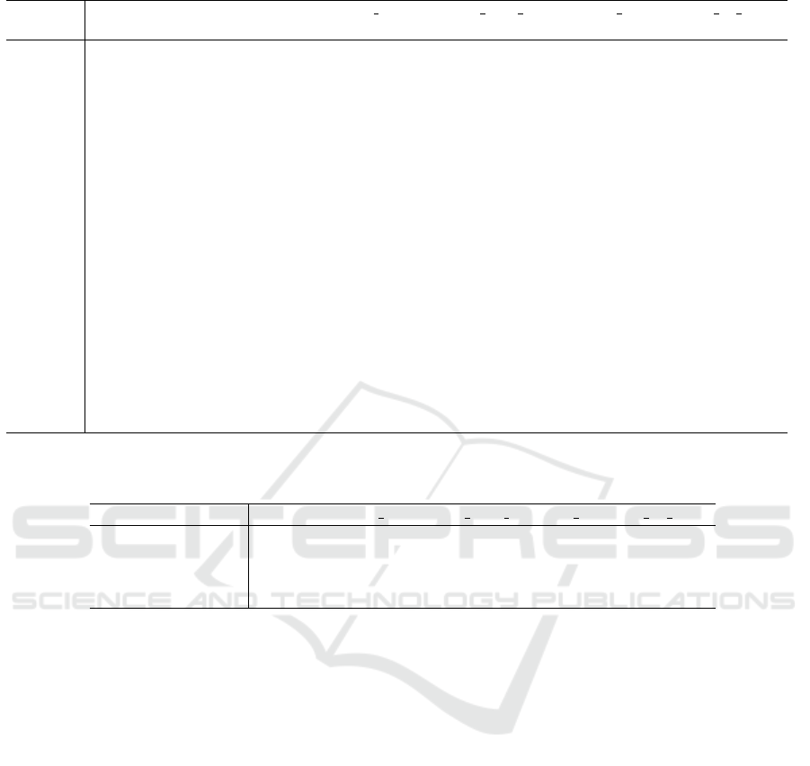
Table 5: Methods performance comparison grouping by instances (number of instances, out of 12, solved to optimality).

Instance milp cp ccg milp ccg milp cp ccg cp ccg cp milp

#Solv. t(s) #Solv. t(s) #Solv. t(s) #Solv. t(s) #Solv. t(s) #Solv. t(s)

SFJS1 12 0.04 12 0.03 12 0.06 12 0.98 12 1.13 12 0.05

SFJS2 12 0.03 12 0.03 12 0.03 12 0.25 12 0.38 12 0.04

SFJS3 12 0.4 12 0.08 12 0.5 12 3.03 12 3.17 12 0.11

SFJS4 12 0.25 12 0.05 12 0.23 12 1.65 12 1.77 12 0.08

SFJS5 12 0.83 12 0.12 12 1.03 12 2.93 12 3.8 12 0.2

SFJS6 12 4.55 12 0.44 12 1.49 12 5.62 12 4.89 12 0.25

SFJS7 12 1.3 12 0.25 12 0.31 12 1.46 12 1.73 12 0.11

SFJS8 12 7.32 12 0.62 12 1.79 12 5.68 12 6.22 12 0.31

SFJS9 12 11.5 12 2.05 12 1.42 12 2.47 12 3.19 12 0.16

SFJS10 12 128 12 3.1 12 2.01 12 8.59 12 11.5 12 0.2

MFJS1 6 1115 6 1445 12 257 12 297 12 73.1 12 19.9

MFJS2 4 1246 6 858 12 161 12 199 12 44.6 12 9.55

MFJS3 0 - 1 1301 11 549 10 414 11 174 12 99.5

MFJS4 0 - 0 - 5 849 5 1715 11 539 11 450

MFJS5 0 - 0 - 5 694 6 1089 10 544 10 328

MFJS6 0 - 0 - 2 1643 1 2522 7 255 9 739

MFJS7 0 - 0 - 0 - 0 - 4 1006 4 815

MFJS8 0 - 0 - 0 - 0 - 3 1144 3 880

MFJS9 0 - 0 - 0 - 0 - 0 - 0 -

MFJS10 0 - 0 - 0 - 0 - 0 - 0 -

Table 6: Methods performance comparison grouping by uncertainty budget (number of instances, out of 60, solved to opti-

mality).

Uncertainty budget milp cp ccg milp ccg milp cp ccg cp ccg cp milp

20 % 35 37 38 38 42 42

40 % 30 31 39 39 45 48

60 % 30 30 42 43 49 49

80 % 35 35 48 46 54 54

methods according to the given uncertainty budget.

We notice that for the extended methods, the resolu-

tion is more difﬁcult for medium budget (40 % and

60 %); this is due to the fact that these uncertainty

budgets generate a greater number of scenarios and,

in these methods, the number of decision variables is

directly related to the number of scenarios. However,

for methods based on the column and constraint gen-

eration algorithm, the number of instances solved to

optimality increases with the uncertainty budget. It

shows that the number of scenarios has no direct ef-

fect on the difﬁculty of the problem.

6 CONCLUSIONS

In this paper, we consider the two-stage ﬂexible job-

shop scheduling problem where the operation pro-

cessing times are subject to uncertainty. The ﬁrst

stage is devoted to ﬁxing the assignment and sequenc-

ing decisions; the second stage determines the start

time of the operations.

As a main contribution, we introduce two robust

counterpart formulations to solve the robust schedul-

ing problem, including one based on constraint pro-

gramming. We use a column and constraint gener-

ation algorithm mixing both integer linear program-

ming and constraint programming. Experimental re-

sults show that the best method, among those tested

in this study, is the constraint and column generation

method using constraint programming in the master

problem and an integer linear programming model for

the subproblem.

REFERENCES

Ben-Tal, A., El Ghaoui, L., and Nemirovski, A. (2009). Ro-

bust optimization, volume 28. Princeton university

press.

Ben-Tal, A., Goryashko, A., Guslitzer, E., and Nemirovski,

A. (2004). Adjustable robust solutions of uncer-

tain linear programs. Mathematical Programming,

99(2):351–376.

Bertsimas, D. and Sim, M. (2004). The price of robustness.

Hybrid Methods to Solve the Two-Stage Robust Flexible Job-Shop Scheduling Problem with Budgeted Uncertainty

141

Operations Research, 52(1):35–53.

Brandimarte, P. (1993). Routing and scheduling in a ﬂex-

ible job shop by tabu search. Annals of Operations

Research, 41(3):157–183.

Dauz

ere-P

es, S. and Paulli, J. (1997). An integrated ap-

proach for modeling and solving the general multipro-

cessor job-shop scheduling problem using tabu search.

Annals of Operations Research, 70:281–306.

Duarte, J. L. R., Fan, N., and Jin, T. (2020). Multi-process

production scheduling with variable renewable inte-

gration and demand response. European Journal of

Operational Research, 281(1):186–200.

Fattahi, P., Mehrabad, M. S., and Jolai, F. (2007). Mathe-

matical modeling and heuristic approaches to ﬂexible

job shop scheduling problems. Journal of Intelligent

Manufacturing, 18(3):331–342.

Garey, M. R., Johnson, D. S., and Sethi, R. (1976).

The complexity of ﬂowshop and jobshop scheduling.

Mathematics of Operations Research, 1(2):117–129.

Hamaz, I., Houssin, L., and Caﬁeri, S. (2018). The cyclic

job shop problem with uncertain processing times.

In 16th International Conference on Project Manage-

ment and Scheduling (PMS 2018), pages 119–122,

Rome, Italy.

Kress, D. and M

uller, D. (2019). Mathematical models for

a ﬂexible job shop scheduling problem with machine

operator constraints. IFAC-PapersOnLine, 52(13):94–

99.

Levorato, M., Figueiredo, R., and Frota, Y. (2022). Exact

solutions for the two-machine robust ﬂow shop with

budgeted uncertainty. European Journal of Opera-

tional Research, 300(1):46–57.

Shen, L., Dauz

ere-P

es, S., and Neufeld, J. S. (2018).

Solving the ﬂexible job shop scheduling problem with

sequence-dependent setup times. European Journal of

Operational Research, 265(2):503–516.

Silva, M., Poss, M., and Maculan, N. (2020). Solution al-

gorithms for minimizing the total tardiness with bud-

geted processing time uncertainty. European Journal

of Operational Research, 283(1):70–82.

Soyster, A. L. (1973). Convex programming with set-

inclusive constraints and applications to inexact lin-

ear programming. Operations Research, 21(5):1154–

1157.

Zeng, B. and Zhao, L. (2013). Solving two-stage robust

optimization problems using a column-and-constraint

generation method. Operations Research Letters,

41(5):457–461.

ICORES 2023 - 12th International Conference on Operations Research and Enterprise Systems

142