Reinforcement Learning Explained via Reinforcement Learning:
Towards Explainable Policies through Predictive Explanation
L
´
eo Sauli
`
eres
a
, Martin C. Cooper
b
and Florence Bannay
c
IRIT, University of Toulouse III, France
Keywords:
Explainable Artificial Intelligence, Reinforcement Learning.
Abstract:
In the context of reinforcement learning (RL), in order to increase trust in or understand the failings of an
agent’s policy, we propose predictive explanations in the form of three scenarios: best-case, worst-case and
most-probable. After showing W[1]-hardness of finding such scenarios, we propose linear-time approxima-
tions. In particular, to find an approximate worst/best-case scenario, we use RL to obtain policies of the
environment viewed as a hostile/favorable agent. Experiments validate the accuracy of this approach.
1 INTRODUCTION
Over the last few years, eXplainable Artificial In-
telligence (XAI) has become a prominent research
topic. This field especially grew up in reaction to
the need to explain black-box AI models. The need
for such explanations has been emphasized by re-
searchers (Lipton, 2018; Darwiche, 2018) but also by
(European Commission, 2021). Automated explain-
ers can lead to more trustworthy AI-models which can
then be used in more applications, including high risk
or safety-critical applications.
The aim of this paper is to make progress in the
search for explainers in the domain of Reinforcement
Learning (RL). RL can be summarized as follows. An
agent learns to make a sequence of decisions consist-
ing of actions within an environment. At each time-
step, the information available to the agent defines a
state. In a state, the agent chooses an action, and
so arrives in a new state, determined by a transition
function (which is not necessarily deterministic), and
receives a reward (a negative reward being rather a
punishment). The agent aims at maximizing its re-
ward, while striking a balance between exploration
(discover new ways to face the problem) and exploita-
tion (use already learnt knowledge). The agent’s strat-
egy is learnt in the form of a policy, which maps each
state to either an action (if the policy is deterministic)
or a probability distribution over actions (if the policy
a
https://orcid.org/0000-0002-4800-9181
b
https://orcid.org/0000-0003-4853-053X
c
https://orcid.org/0000-0001-7891-9920
is stochastic).
Explainable Reinforcement Learning (XRL) is a
subdomain of XAI which focuses on providing ex-
planations for RL. Several XRL approaches already
exist based on different key features of RL. For exam-
ple, the VIPER algorithm (Bastani et al., 2018) learns
a Decision Tree policy which is a surrogate for the
actual policy given by a deep neural network. The
surrogate policy is easier to verify concerning differ-
ent properties such as safety, stability and robustness.
Another approach is reward decomposition (Juoza-
paitis et al., 2019) which focuses on the reward func-
tion and is used when an agent has multiple objec-
tives. This XRL method expresses a reward through
a vector of scalars instead of a simple scalar. This
makes it easier to understand why an agent performs
an action, and to identify its objective in choosing this
action. A third example of approach is proposed in
(Greydanus et al., 2018) and uses the fact that the cur-
rent state of an agent can be assimilated to the input
of a classifier, where the policy is the classifier and
the action chosen is the class. With this in mind, the
XRL method of Greydanus et al. generates saliency
maps on images with a perturbation-based approach.
A saliency map consists in highlighting parts of the
image (in this case images from an Atari 2600 game)
that lead the agent to choose an action.
In their survey, Milani et al. emphasize the need
for explanations that capture the concepts of RL (Mi-
lani et al., 2022). Our study tries to meet this need
by proposing a predictive XRL method based on the
sequential aspect of RL. The aim of this method is to
answer the question “What is likely to happen from
Saulières, L., Cooper, M. and Bannay, F.
Reinforcement Learning Explained via Reinforcement Learning: Towards Explainable Policies through Predictive Explanation.
DOI: 10.5220/0011619600003393
In Proceedings of the 15th International Conference on Agents and Artificial Intelligence (ICAART 2023) - Volume 2, pages 35-44
ISBN: 978-989-758-623-1; ISSN: 2184-433X
Copyright
c
 2023 by SCITEPRESS – Science and Technology Publications, Lda. Under CC license (CC BY-NC-ND 4.0)
35

the state s with the current policy of the agent?”. To
this end, we compute three different state-action se-
quences (called scenarios), starting from the current
state s. This method allows us to explain a policy by
giving pertinent examples of scenarios from s, hence
the name of the explainer: Scenario-Explanation,
shortened to SXp. It provides information about fu-
ture outcomes by looking forward k time-steps ac-
cording to three different scenarios: a worst-case sce-
nario, a most-probable scenario and a best-case sce-
nario. To avoid an exhaustive search over all possi-
ble scenarios, we propose approximations based on
learning policies of hostile/favorable environments.
Our approximate SXp’s are computed using transi-
tion functions learnt by treating the environment as an
RL agent. The advantage is that this can be achieved
by using the same technology and the same compu-
tational complexity as the learning of the agent’s pol-
icy. We tested our approximate SXp on two problems:
Frozen Lake, an Open AI Gym benchmark problem
(Brockman et al., 2016), and Drone Coverage, a prob-
lem we designed.
This paper first gives a theoretical justification for
Scenario-Explanation, before describing experimen-
tal results on two RL problems. It then surveys re-
lated work on XRL, before discussing the efficiency
and usefulness of SXp.
2 SCENARIO-EXPLANATION
Before describing our XRL method, we need to intro-
duce some notation. An RL problem is described by a
Markov Decision Process (MDP) (Sutton and Barto,
2018). An MDP is a tuple hS,A,R, pi where S and A
are respectively the state and action space, R : S×A →
R is the reward function, p : S × A → Pr(S) is the
transition function of the environment which provides
a distribution over reachable states: given an action
a ∈ A and a state s ∈ S, p(s
0
|s,a) denotes the proba-
bility to reach the state s
0
when a is performed in the
state s. For a deterministic policy π : S → A,π(s) de-
notes the action the agent performs in s whereas for
a stochastic policy π : S → Pr(A), π(a|s) denotes the
probability that the agent performs action a in s.
Our aim is to answer the question: “What is likely
to happen from the state s with the current policy
of the agent?”. We choose to do this by providing
three specific scenarios using the learnt policy π. By
scenario, we mean a sequence of states and actions,
starting with s. Scenarios are parameterised by their
length, denoted by k, which we consider in the fol-
lowing as a constant. We provide a summary of all
possible scenarios via the most-probable, the worst-
case and the best-case scenarios starting from s.
When considering possible scenarios, we may
choose to limit our attention to those which do not
include highly unlikely transitions or actions. The fol-
lowing technical definition based on two thresholds α
and β allows us to restrict the possible transitions and
actions. We do not filter out all transitions with prob-
ability less than a certain threshold, but rather those
whose probability is small (less than a factor of α)
compared to the most likely transition. This ensures
that at least one transition is always retained. A sim-
ilar remark holds for the probability of an action. We
filter out those actions whose probability is less than a
factor of β from the probability of the most probable
action.
Definition 1. Given k ∈ N
∗
, α,β ∈ [0,1], an MDP
hS,A, R, pi and a stochastic policy π over S, an
(α,β)-credible length-k scenario is a state-action se-
quence s
0
,a
0
,s
1
,a
1
,..., a
k−1
,s
k
∈ (S × A)
k
× S which
satisfies: ∀i ∈ {0, ...,k−1}, π(a
i
|s
i
)/π
∗
≥ β and
p(s
i+1
|s
i
,a
i
)/p
∗
≥ α, where π
∗
= max
a∈A
π(a|s
i
) and
p
∗
= max
s∈S
p(s|s
i
,a
i
).
In a (1,1)-credible length-k scenario, the agent al-
ways chooses an action among it’s most likely choices
and we only consider the most probable transitions
of the environment. At the other extreme, in a (0,0)-
scenario, there are no restrictions on the choice of ac-
tions or on the possible transitions of the environment.
The following definition is parameterised by
α,β ∈ [0, 1] and an integer k. For simplicity of presen-
tation, we leave this implicit and simply write credible
scenario instead of (α, β)-credible length-k scenario.
In the following definition, R(σ) denotes the reward
of a credible scenario σ. By default R(σ) is the re-
ward attained at the last step of σ.
Definition 2. For an MDP hS,A, R, pi and a policy π
over S, a scenario-explanation for π from a state s is
a credible scenario σ = s
0
,a
0
,s
1
,a
1
,..., a
k−1
,s
k
such
that s
0
= s.
σ is a most-probable scenario-explanation for π
from s if its probability given s, denoted Pr(σ), is
maximum, where
Pr(σ) =
k
∏
i=1
π(a
i−1
|s
i−1
)p(s
i
|s
i−1
,a
i−1
)
σ is a best-case scenario-explanation for π from s
if it maximises the reward R(σ). σ is a worst-case
scenario-explanation from s if it minimizes the re-
ward R(σ).
In the best (worst) case, the environment always
changes according to the best (worst) transitions for
the agent, i.e., the environment maximises (min-
imises) the agent’s reward after k steps. Not surpris-
ICAART 2023 - 15th International Conference on Agents and Artificial Intelligence
36

ingly, finding such scenarios is not easy, as we now
show.
Proposition 1. For any fixed values of the parame-
ters α,β ∈ [0, 1], the problem of finding a best-case or
worst-case length-k scenario-explanation, when pa-
rameterized by k, is W[1]-hard. Finding a most-
probable length-k scenario-explanation is W[1]-hard
provided α < 1.
Proof. It suffices to give a polynomial reduction from
CLIQUE which is a well-known W[1]-complete prob-
lem (Downey and Fellows, 1995). We consider a
Markov decision process concerning an agent who
can move along edges of a n-vertex graph G. Vis-
ited vertices are colored red, whereas unvisited ver-
tices are green. The state is the position of the agent
together with the list of red vertices. Transitions (de-
termined by the environment) are given by random
moves along edges to a vertex adjacent to the cur-
rent vertex. All transitions are equally likely, so they
are all possible whatever the value of α (the lower
bound on the likelihood of transitions compared to
the most-probable transition). Suppose that the pol-
icy of the agent is simply to remain still. Since this
policy is deterministic, the value of the parameter β
(the lower bound on the probability of actions) has
no effect on the set of actions to consider. In this
setting, a sequence of states ending with a state s
k
with k + 1 visited vertices can be associated to a
length-k scenario explanation σ = s
0
,a
0
,. .., a
k−1
,s
k
where each action a
i
is to remain still. The reward
R(σ) of a length-k scenario explanation is defined by
R(σ) =

k+1
2

− e(s
k
) where e(s
k
) is the number of
edges between the red vertices listed in the state s
k
(i.e. R is the number of missing edges to obtain a
clique composed of the k+1 visited vertices). We can
see that a worst-case length-k scenario leads to a re-
ward of 0 iff G contains a (k+1)-clique including the
start vertex. We can apply the same proof to the best-
case length-k scenario by simply setting the reward to
be −R(σ).
We can adapt the same proof to the case of the
most-probable scenario by changing the transition
probabilities. We consider an edge to be red if both
its vertices are red. Transitions which add r new
red edges to a graph already containing r red ver-
tices has probability q, and all other transitions prob-
ability p. Since α < 1, we can choose p,q so that
α < p/q < 1. This means again that all transitions are
possible in (α, β)-credible scenarios, but that a most-
probable length-k scenario (of probability q
k
) colors
a (k+1)-clique including the start vertex iff such a
clique exists in G.
2.1 Approximate Scenario-Explanation
In view of Proposition 1, we consider approxima-
tions to scenario-explanations which we obtain via
an algorithm whose complexity is linear in k, the
length of the SXp. Indeed, since determining most-
probable/worst/best scenarios is computationally ex-
pensive, we propose to approximate them. For this
purpose, it can be useful to imagine that the environ-
ment acts in a deliberate manner, as if it were another
agent, rather than in a neutral manner according to a
given probability distribution. In this paper, as a first
important step, we restrict our attention to approxi-
mate SXp’s that explain deterministic policies π.
An environment policy π
e
denotes a policy that
models a specific behavior of the environment. There
are different policies π
e
for the most-probable, worst
and best cases which correspond to policies of neu-
tral, hostile and favorable environments respectively.
In the case of a hostile/favorable environment, π
e
de-
notes an environment policy that aims at minimiz-
ing/maximizing the reward of the agent. The policy
of a neutral environment is already given via the tran-
sition probability distribution p. On the other hand
the policies of hostile or favorable environments have
to be learnt. We propose to again use RL to learn
these two policies. Compared to the learning of the
agent’s policy, there are only fairly minor differences.
Clearly, in general, the actions available to the envi-
ronment are not the same as the actions available to
the agent. Another technical detail is that as far as the
environment is concerned the set of states is also dif-
ferent, since its choice of transition depends not only
on the state s but also on the action a of the agent.
Recall, from Definition 1, that in a (1,1)-scenario
a most-probable action and a most-probable transition
are chosen at each step. Of course, for determinis-
tic policies or transition functions there is no actual
choice.
Definition 3. A probable scenario-explanation (P-
scenario) of π from s is a (1,1)-scenario for π starting
from s.
A favorable-environment scenario-explanation
(FE-scenario) for π from s is a (1,1)-scenario, in
which the transition function (p in Definition 1) is a
learnt policy π
e
of a favorable environment.
A hostile-environment scenario-explanation (HE-
scenario) for π from s is a (1,1)-scenario, in which the
transition function p is a learnt policy π
e
of a hostile
environment.
A length-k P-scenario is computed by using an al-
gorithm that simply chooses, at each of k steps start-
ing from the state s, the action determined by π and a
most-probable transition according to p. In the case
Reinforcement Learning Explained via Reinforcement Learning: Towards Explainable Policies through Predictive Explanation
37

of the FE/HE scenario, p is replaced by the environ-
ment policy π
e
which is learnt beforehand. The same
RL method that was used to learn the agent’s policy
π is used to learn π
e
(which hence is deterministic
since we assume that π is deterministic). The fact
that the learnt environment policy π
e
is deterministic
means that scenario-explanations can be produced in
linear time. In the favorable-environment (FE) case
the reward for the environment is R (the same func-
tion as for the agent) and in the hostile-environment
(HE) case the reward function is (based on) −R.
Proposition 2. Consider an MDP hS,A, R, pi for
which we learn by RL a deterministic policy π. Pro-
ducing length-k P/HE/FE scenario-explanations does
not increase the asymptotic worst-case (time and
space) complexity of the training phase. Moreover
the computation of the explanation only incurs a cost
which is linear in k.
Proof. By design, we use the same RL method (sub-
ject to the same constraints on computational re-
sources) to learn π
e
as was used to learn π. This en-
sures that the asymptotic worst-case time complexity
of the training phase does not increase. However, in
tabular methods there is a risk that space complex-
ity increases due to the fact that when learning π
e
environment-states are pairs (s, a) ∈ S × A. We say
that (s,a) is π-reachable if it can be encountered dur-
ing the execution of the policy π by the agent. For
a deterministic policy π, there is a unique action a
π,s
that the agent can execute when in state s, so the set
of π-reachable environment-states (s, a) is in bijection
with S. It follows that space complexity of the train-
ing phase also does not increase. The production of
a P/HE/FE-scenario is clearly linear in k since deter-
mined by π and p or π
e
.
Having shown that our algorithm is efficient in
time, hence avoiding the complexity issue raised by
Proposition 1, in the following section we describe
experiments which indicate that the returned results
are good approximations of the most-probable, best
and worst explanations.
3 EXPERIMENTAL RESULTS
The Frozen Lake (FL) and Drone Coverage (DC)
problems illustrate, respectively, a single and a multi-
agent context. Furthermore, the training process was
managed by two distinct algorithms, respectively Q-
learning (Watkins and Dayan, 1992) and a Deep-Q-
Network (Mnih et al., 2015). Recall that the algorithm
used to train environment-agents is similar to the one
used to train the agent.
The exploration/exploitation trade-off is achieved
by using an ε-greedy action selection where ε is
a probability to explore. The hyper-parameter k
(scenario-length) is set to 5 and 6 respectively for
the FL and DC problems. FL experiments were run
on a ASUS GL552VX, with 8 GB of RAM and a
2.3GHz quad-core i5 processor and DC experiments
were carried out using a Nvidia GeForce GTX 1080
TI GPU, with 11 GB of RAM (source code available
on: https://github.com/lsaulier/SXp-ICAART23).
To measure the SXp produced, we did not find in
the literature a metric for this specific type of explana-
tion. That is why we implemented three simple scores
to answer the question: “How good is the generated
Scenario-Explanation?”. Let the function f denote
the quality evaluation function of a scenario σ; f (σ)
can vary depending on the application domain and the
quality aspect we choose to measure. By default it is
equal to the reward R(σ), but may be refined to incor-
porate other criteria for technical reasons explained
later. f (σ
F
) and f (σ
H
) are respectively the quality
of a FE-scenario σ
F
and a HE-scenario σ
H
. They are
used to measure to what extent the scenario is similar
to a best-case or worst-case scenario respectively. The
resulting FE-score/HE-score is the proportion of n
randomly-generated scenarios that have a not strictly
better/worse quality (measured by f ) than the FE/HE-
scenarios themselves (hence the score lies in the range
[0,1]). For the P-scenario, the P-score is the absolute
difference between the normalized quality f (σ
P
) of a
P-scenario σ
P
and the normalized mean of f (σ) of
n randomly-generated scenarios (hence again lies in
the range [0,1]). Formally, given a FE-scenario σ
F
, a
HE-scenario σ
H
and a P-scenario σ
P
from s:
FE-score(σ
F
) =
card({σ ∈ S
n
s
and f (σ) ≤ f (σ
F
)})
n
HE-score(σ
H
) =
card({σ ∈ S
n
s
and f (σ) ≥ f (σ
H
)})
n
P-score(σ
P
) =





norm( f (σ
P
)) − norm(
∑
σ∈S
n
s
f (σ)/n)





where S
n
s
is a set of n randomly-generated sce-
narios s.t. ∀σ = (s
0
,a
0
,. .., s
k
) ∈ S
n
s
, s
0
= s, card
is the cardinality of a set and norm is a function
with argument a value b and based on the minimum
and maximum values of f , denoted b
min
and b
max
:
norm(b) = (b−b
min
)/(b
max
−b
min
). The closer the
HE-score, FE-score of a HE/FE-scenario is to 1, the
closer it is respectively to the worst/best-case sce-
nario because no other, among the n scenarios pro-
duced, is worse/better. A P-score close to 0 indi-
cates that the P-scenario is a good approximation to
ICAART 2023 - 15th International Conference on Agents and Artificial Intelligence
38

an average-case scenario. In each case, the scenar-
ios randomly-generated for comparison are produced
using the agent’s learnt policy π and the transition
function p. As mentioned above, by default, the
function f is the last-step reward of a scenario, i.e.
f (σ) = R(s
k−1
,a
k−1
).
The explanation scores in Tables 1 and 2 are based
on n = 10000 to reduce the randomness of score cal-
culation. The Avg
i
and σ
i
columns show the average
and standard deviation of explanation scores based on
i different states, or configurations (i.e. states of all
agents in a multi-agent problem such as DC).
3.1 Frozen Lake (FL)
3.1.1 Description
The FL problem is an episodic RL problem with dis-
crete state and action spaces. The agent (symbolized
in Figure 2 by a blue dot) moves in a 2D grid world,
representing the surface of a frozen lake, with the aim
to reach an item in a specific cell of the grid (marked
with a star). There are holes in the frozen lake (sym-
bolized by grey cells in the map) and the others cells
are solid ice. When an agent falls into a hole, it loses.
The agent’s initial state is at the top-left corner cell of
the map.
A state is represented by a single value, corre-
sponding to the agent’s position in the map, S =
{1,. .., l × c} with, l, c the map’s dimensions. For
the sake of readability, in the results a state is denoted
by the agent’s coordinates (line,column), where (1, 1)
is the top left cell and (4, 4) is the bottom right cell
which are respectively the initial state of the agent and
its goal on the 4 ×4 map in Figure 2. The action space
is A = {le f t, down, right, up}. The reward function is
sparse and described as follows: for s ∈ S,a ∈ A, s
0
de-
noting the state reached by performing action a from
s, and s
g
being the goal state:
R(s,a) =

1, if s
0
= s
g
.
0, otherwise.
The transition function p is the same from any
state. Because of the slippery nature of the frozen
lake, if the agent chooses a direction (e.g. down), it
has 1/3 probability to go on this direction and 1/3 to
go towards each remaining direction except the oppo-
site one (here, 1/3 to go left and 1/3 to go right).
To solve this RL problem, we use the tabular Q-
learning method because the state and action space is
small. The end of an episode during training is char-
acterized by the agent reaching its goal or falling into
a hole.
As stated in the proof of Proposition 2, an
environment-agent’s state contains an extra piece of
information compared to an agent’s state: the action
executed by the agent from this position, according
to its policy π. As the environment-agent reflects the
transitions of the environment, there are only 3 ac-
tions available and they depend on the agent’s choice
of action. The reward function of the favorable agent
is similar to the agent’s reward function. The hostile
agent receives a reward of 1 when the agent falls into
a hole, of -1 if the agent reaches its goal and a reward
of 0 otherwise.
3.1.2 Results
In order to test our approximate SXp on different en-
vironment sizes, we used a 4 × 4 map and a 8 × 8
map, the ones presented in Open AI Gym (Brock-
man et al., 2016). Since the reward is sparse (0 ex-
cept in goal states), FE/HE/P-scores computed purely
with f (σ) = R(s
k−1
,a
k−1
) are uninformative (when
the number of steps k is not large enough to reach the
goal). Accordingly, the quality evaluation function
was defined as follow: f (σ) = R(σ) + λQ(σ), where
Q(σ) = max
a
k
∈A
Q(s
k
,a
k
) is the maximum last-step
Q-value, R(σ) = R(s
k−1
,a
k−1
) is the reward of sce-
nario σ and λ < 1 is a positive constant. Another par-
ticularity of this problem, is that since the transitions
are equiprobable, many P-scenarios are possible.
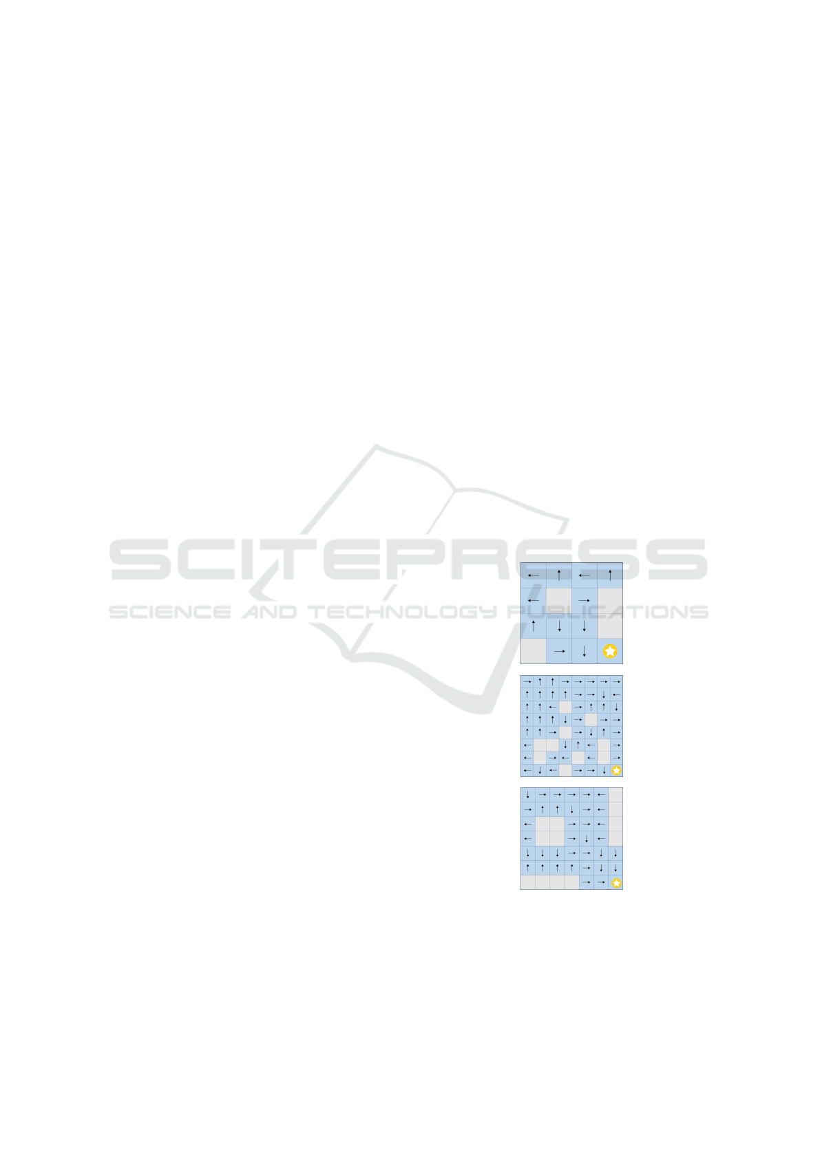
Figure 1: Agent’s learnt policies for the 4 × 4 and 8 × 8
maps of Figure 2 and a safe 7 ×7 grid.
The agent’s learnt policy for the 4 × 4 map is rep-
resented in Figure 1. Each arrow represents the action
performed by the agent from this state. We note that
Reinforcement Learning Explained via Reinforcement Learning: Towards Explainable Policies through Predictive Explanation
39

Table 1: Scores for Scenario-Explanation in the 4 × 4 map
and 8 ×8 map.
4x4 map 8x8 map
State (2,1) Avg
7
σ
7
State (3,6) Avg
20
σ
20
FE-score 1 1 0 1 0.824 0.281
HE-score 1 1 0 1 0.828 0.346
P-score 0.081 0.211 0.115 0.031 0.08 0.09
the agent learns to avoid to enter the top-right part of
the map (i.e. the two first lines without the first col-
umn), which is the most dangerous part, due to the
(2,3) state. In the remaining parts of the map, the
only dangerous state is (3,3) since the agent action
choice is down, so it has a probability of
1
3
to fall into
a hole.
The SXp calculated starting from the state (2,1) is
shown on the left of in Figure 2. The P-scenario is one
scenario among many, and it highlights the difficulty
for the agent to succeed in this particular grid with a
few steps. The hostile agent exploits well its only way
to force the agent to fall into a hole given the agent’s
policy (Figure 1) which is to push it towards the hole
located at (3, 4). The favorable agent also learns well
and provides an FE-scenario where the agent reaches
its goal in the minimum number of steps. The HE-
score and FE-score of SXp’s from state (2,1) are pre-
sented in Table 1. These are perfect scores (equal to
1). Moreover, since the P-score is close to 0, the pro-
vided P-scenario is a good approximation. We com-
puted SXp’s based on the same agent’s policy π but
starting from 7 reachable states, i.e. states that can be
reached following the policy π (Figure 1) and which
are neither holes nor the goal. Results are reported
in the Avg
7
column of Table 1. Hostile and favorable
agents learnt perfectly.
The SXp method was also tested with a 8×8 map.
As we can see in the second grid of Figure 1, the
agent has learned to avoid as much as possible the
left zone of the map which is dangerous. Figure 2
depicts an SXp starting from the state (3, 6). Due to
the agent’s policy, the hostile agent can’t just push the
agent down from state (3,6), but it manages to push
the agent along a path which ensures that the agent
falls into a hole, hence the HE-scenario ends after
only 3 steps. In the FE-scenario, the favorable agent
brings the agent closer to its goal over the k = 5 time-
steps. The P-scenario again provides evidence that the
agent is likely not to succeed in this difficult environ-
ment in a small number of steps. From the scores pre-
sented in Table 1 concerning the 8 × 8 map, we can
again conclude that the 3 produced scenarios are of
good quality. The scores presented in the Avg
20
col-
umn were obtained by SXp from 20 randomly-chosen
starting states. The average score is lower than 1 but
note that 1 is achieved for respectively more than 75%
and 60% of HE-scenarios and FE-scenarios. Hence,
apart from some randomly-generated starting states
located in the little explored left-zone of the map,
the scores indicate that HE/FE-scenarios are good ap-
proximations of worst/best scenarios.
In order to check the impact of the agent’s policy
on the environment-agents’ learning process, we de-
signed a 7 × 7 map, shown in Figure 1, in such a way
that if the agent learns well, it can avoid falling into
a hole. Once the learning phase is over, we noticed
that the hostile agent learns nothing. Since the agent
learns an optimal policy π, the hostile agent can’t push
the agent into a hole. Accordingly, it can’t receive any
positive reward and therefore can’t learn state-action
values. This is strong evidence that the agent’s policy
is good.
3.2 Drone Coverage (DC)
3.2.1 Description
The DC problem is a novel multi-agent, episodic RL
problem with discrete state and action spaces. The
agents’ goal is to cover the largest area in a windy 2D
grid-world containing trees (symbolized by a green
triangle in Figure 3). The coverage of each drone
(represented as a dot) is a 3 × 3 square centered on
its position. A drone is considered as lost and indeed
disappears from the grid if it crashes into a tree or an-
other drone.
A state for an agent is composed of the contents
of its neighbourhood (a 5 × 5 matrix centered on the
agent’s position) together with its position on the map.
The action space is A = {left,down,right,up,stop}.
The reward function R of an agent is impacted by
its coverage, its neighbourhood, and whether it has
crashed or not (the reward is -3 in case of crash): if
there is no tree or other drone in the agent’s 3 ×3 cov-
erage, it receives a reward (called cover) of +3 and
+0.25 × c otherwise, where c is the number of free
cells (i.e. with no tree or drone) in its coverage; the
agent receives a penalty of −1 per drone in its 5 × 5
neighbourhood (since this implies overlapping cover-
age of the two drones). With s
0
the state reached by
executing action a from s, the reward function is as
follows: for s ∈ S,a ∈ A,
R(s,a) =

−3, if crash
cover(s
0
) + penalty(s
0
), otherwise
As there are 4 drones, the maximum cumula-
tive reward (where cumulative reward means the sum
of all agents rewards in a given configuration) is
ICAART 2023 - 15th International Conference on Agents and Artificial Intelligence
40

Figure 2: Scenario-Explanations from a specific state (on the left of each SXp) in the 4× 4 map and 8×8 map. The three lines
correspond respectively to the FE-scenario, HE-scenario and P-scenario. No more states are displayed in the HE-scenarios
after a terminal state is attained in which the agent has fallen in a hole.
12 and the minimum is −12. The transition func-
tion p, which represents the wind, is similar in each
position and is given by the following distribution:
[0.1,0.2, 0.4,0.3]. This distribution defines the proba-
bility that the wind pushes the agent respectively left,
down, right, up. After an agent’s action, it moves
to another position and then is impacted by the wind.
As an additional rule, if an agent and wind directions
are opposite, the agent stays in its new position, so the
wind has no effect. After a stop action, the drone does
not move and hence is not affected by the wind.
In order to train the agents, we used the first ver-
sion of Deep-Q Networks (Mnih et al., 2015) com-
bined with the Double Q-learning extension (Hasselt,
2010). The choice of this algorithm was motivated
by two factors. First, we wanted to investigate our
XRL method’s ability to generalise to RL algorithms,
such as neural network based methods, used when the
number of states is too large to be represented in a
table. Secondly, this setting enables us to deal with
a problem which is scalable in the number of drones
and grid size.
The end of an episode of the training process oc-
curs when either one agent crashes, or a time horizon
is reached. This time horizon is a hyper-parameter
fixed before the training; it was set to 22 for the train-
ing of the policy which is explained in the following
subsection. When restarting an episode, the agents’
positions are randomly chosen. This DC problem is a
multi-agent problem, and to solve it, we use a naive
approach without any cooperation between agents.
Only one Deep-Q Network is trained with experi-
ences from all agents. The reward an agent receives is
only its own reward; we do not use a joint multi-agent
reward.
Concerning the implementation of the hostile and
favorable environment: the extra information in the
environment-agent’s state is the action performed by
the agent in its corresponding state. Actions are sim-
ilar to the agents’ except that there is no stop action.
The favorable-agent reward function is similar to the
one of the agent’s and the reward function of the hos-
tile agent is exactly the opposite.
3.2.2 Results
For the sake of simplicity, each drone has an associ-
ated color in Figure 3. Above each map, there is a
list of colored arrows, or stop symbols, correspond-
ing to each colored drone’s action which leads them
to the configuration displayed in the map. A colored
cell means that the area is covered by the drone of the
same color and a dark grey cell indicates an overlap of
the coverage of different drones. To compute the SXp
scores, we use f (σ) =
∑
i
R
i
(s
k−1
,a
k−1
) with R
i
denot-
ing the reward of agent i (i.e. f is the last-step aggre-
gate reward). Note that the policy to be explained is
good, but not optimal. Measuring the performance of
a policy by the average of the cumulative rewards ob-
tained at the end of the last hundred training episodes,
the performance is 11.69 (out of 12).
The SXp for a particular configuration, denoted
as configuration A, is shown in Figure 3. The hostile
agent succeeds in crashing two drones and position-
ing the remaining drones in bad covering positions.
The P-scenario demonstrates well the most probable
transition (the wind pushes the drones to the right)
and the favorable agent manages to reach a perfect
configuration in only 5 steps. Results are given in Ta-
ble 2 where the last columns show the average and
standard deviation of scores obtained from 30 random
configurations. These results indicate good approxi-
mate SXp’s. Moreover experiments showed that 19
HE-scores are higher than 0.95 and 24 FE-scores are
perfect (equal to 1). The quality of the learnt policy
is also attested by the fact that a maximum reward is
attained in 21 out of 30 P-scenarios.
Results obtained in the FL and DC problems show
that, whether the agent’s policy is optimal or not, we
can obtain interesting information via our SXp. Fur-
Reinforcement Learning Explained via Reinforcement Learning: Towards Explainable Policies through Predictive Explanation
41

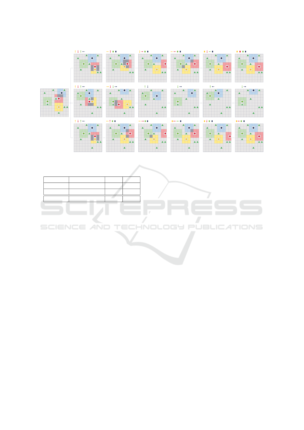
Figure 3: Scenario-Explanation of a specific configuration of the DC problem. The starting configuration A is at the left and
the three lines correspond respectively to the FE-scenario, HE-scenario and P-scenario.
Table 2: Scores for Scenario-Explanation in 10 × 10 map.
Configuration A Avg
30
σ
30
FE-score 1 0.919 0.198
HE-score 1 0.936 0.08
P-score 0.073 0.034 0.04
thermore, this XRL method does not increase asymp-
totic complexity.
4 RELATED WORK
XRL methods use different key features of Reinforce-
ment Learning to provide explanations. As an exam-
ple, we can cite the interpretable reward proposed in
(Juozapaitis et al., 2019). Using exclusively the states,
Greydanus et al. present a method to produce saliency
maps for Atari agents (Greydanus et al., 2018). By
adding object recognition processing, Iyer et al. pro-
duce object saliency maps from states to gain more in-
sights about the agent’s decisions (Iyer et al., 2018)..
In order to focus on causal relationship between ac-
tion and state variables, authors of (Madumal et al.,
2020) build an action influence model used for expla-
nation. Additional information can be collected dur-
ing the agent’s training process, including XRL meth-
ods (Cruz et al., 2019) which extract success proba-
bilities and number of transitions, or methods which
learn a belief map (Yau et al., 2020). All these XRL
methods allow one to essentially explain the choice of
an action in a specific state. For policy-level explana-
tions, EDGE highlights the most critical time-steps,
states, given the agent’s final reward in an episode
(Guo et al., 2021). To create an interpretable pol-
icy in a multi-task RL problem, each policy learned
for a sub-task (corresponding to the general policy’s
actions) can be represented as a human-language de-
scription (Shu et al., 2017).
Another way to explain is through state-action
sequences, like our SXp. One part of the frame-
work proposed by Sequeira and Gervasio provides a
visual summary, based on sequences obtained dur-
ing the learning phase, to globally explain the pol-
icy (Sequeira and Gervasio, 2020). With the same
goal, HIGHLIGHTS extracts sequences based on a
notion of state importance to provide a summary of
the agent’s learnt behaviour (Amir and Amir, 2018).
In a context of MDP, the method implemented in
(Tsirtsis et al., 2021) computes sequences that differ
in at most n actions from the sequence to explain, as
counterfactual explanations. Explaining a sequence
in a contrastive way, is achieved in (van der Waa
et al., 2018) by producing a contrastive policy from
the user question and then comparing both sequences.
These XRL methods do not solve the same problem as
our SXp. Indeed, (Sequeira and Gervasio, 2020) and
(Amir and Amir, 2018) provide high-level policy ex-
planation through summaries in a general context of
the agent’s interaction with the environment. (Tsirt-
sis et al., 2021) and (van der Waa et al., 2018) ex-
plain the policy in a counterfactual way; the problem
is to generate a sequence in which actions differ from
π. Thus, these approaches are incomparable with our
SXp, which explain the policy from a particular state,
by producing scenarios using the policy π.
ICAART 2023 - 15th International Conference on Agents and Artificial Intelligence
42

5 DISCUSSION
The experiments illustrate the different possible uses
of SXp. Apart from understanding policies, SXp also
provide a means to evaluate them. Indeed, even if the
policy π learned is not optimal, HE-scenarios and FE-
scenarios provide useful information. If from multi-
ple starting states, an FE agent cannot bring the agent
closer to its goal, this is a proof that the policy π is
inadequate. Conversely, an HE agent which cannot
prevent the agent from reaching its goal is a evidence
of a good policy π. Concretely, in the FL problem
this means that the agent has learnt not to give a hos-
tile environment the opportunity to force it to fall into
a hole, and in the DC problem the agent learns to stay
sufficiently far away from trees and other drones. In
other words, our XRL method can also be used as a
debugging tool.
The experiments have also taught us some valu-
able lessons. Since we use the same RL method and
the same resources to learn π
e
as were used to learn
π (in order not to increase asymptotic time and space
complexity), we cannot expect quality of explanations
to be better than the quality of the original policy π.
For example, when states are represented by a sim-
ple index in a table, as in Q-learning, π
e
can provide
no useful information concerning states which were
not visited during the learning of π
e
. Indeed, what-
ever the RL method used, since π
e
is learnt after (and
as a function of) the agent’s policy π, the latter will
be of better quality on (states similar to) states visited
more frequently when following the agent’s policy π.
A higher/lower quality of explanation for those states
that are more/less likely to be visited is something the
user should be aware of. If it is important that quality
of explanations should be independent of the proba-
bility of a state, then the training phase of π
e
should
be adapted accordingly. This is an avenue of future
research.
We should point out the limitations of our method.
The three scenarios which are produced are only ap-
proximations to the worst-case, best-case and most-
probable scenarios. Unfortunately, approximation is
necessary due to computational complexity consider-
ations, as highlighted by Proposition 1. We should
also point out that the distinction between these three
scenarios only makes sense in the context of RL prob-
lems with a stochastic transition function. Finally,
due to the relative novelty of the notion of scenario-
explanation, no metric was found in the literature to
evaluate SXp’s.
6 CONCLUSION
In this paper, we describe an RL-specific explanation
method based on the concept of transition in Rein-
forcement Learning. To the best of our knowledge,
SXp is an original approach for providing predictive
explanations. This predictive XRL method explains
the agent’s deterministic policy through scenarios
starting from a certain state. Moreover, SXp is agnos-
tic concerning RL algorithms and can be applied to
all RL problems with a stochastic transition function.
With HE-scenarios and FE-scenarios, we attempt to
bound future state-action sequences. They respec-
tively give an approximation of a worst-case scenario-
explanation and a best-case scenario-explanation. To
compute HE-scenarios and FE-scenarios, we firstly
need to learn respectively a hostile environment’s pol-
icy and a favorable environment’s policy. Our experi-
mental trials indicate that these approximations are in-
formative since close to worst/best-case scenarios and
can be found without exhaustive search. Our XRL
method is completed by the most-probable scenario-
explanation, approximated by the P-scenario. Each
of these three scenarios composing the SXp are com-
puted using the agent’s policy and hence provide a
predictive explanation for the agent’s policy. The
experiments show that SXp leads to a good answer
to the question “What is likely to happen from the
state s with the current policy of the agent?”. Our
3-scenario-based method appears promising and can
be used in more complex problems: we only require
that it is possible to learn policies for hostile/favorable
environments.
This paper points to various avenues of possible
future work. An avenue of future work would be to
focus on the probabilistic aspect of stochastic poli-
cies and provide specific approximate SXp defini-
tions. We chose a small number for the value of the
hyper-parameter k in order to provide succinct user-
interpretable explanations. It is worth noting that in-
creasing k hardly affects computation time (which is
dominated by the training phase). An obvious im-
provement is to use a large k value, but displaying
only the first/last few steps of the scenario, along with
a summary of the missing steps.
Our implementation of SXp can be seen as a proof
of concept. We see SXp as a new tool to add to
the toolbox of XAI methods applicable to RL. We
have tested it successfully on two distinct problems
in which RL was used to learn a deterministic pol-
icy. Of course, in any new application, experimental
trials would be required to validate this approach and
evaluate its usefulness. An avenue of future research
would be to study possible theoretical guarantees of
Reinforcement Learning Explained via Reinforcement Learning: Towards Explainable Policies through Predictive Explanation
43

performance.
In summary, after introducing a theoretical frame-
work for studying predictive explanations in RL, we
presented a novel practical model-agnostic predictive-
explanation method.
REFERENCES
Amir, D. and Amir, O. (2018). HIGHLIGHTS: summariz-
ing agent behavior to people. In Andr
´
e, E., Koenig,
S., Dastani, M., and Sukthankar, G., editors, Pro-
ceedings of the 17th International Conference on Au-
tonomous Agents and MultiAgent Systems, AAMAS,
pages 1168–1176. International Foundation for Au-
tonomous Agents and Multiagent Systems / ACM.
Bastani, O., Pu, Y., and Solar-Lezama, A. (2018). Verifiable
reinforcement learning via policy extraction. In Ben-
gio, S., Wallach, H. M., Larochelle, H., Grauman, K.,
Cesa-Bianchi, N., and Garnett, R., editors, NeurIPS,
pages 2499–2509.
Brockman, G., Cheung, V., Pettersson, L., Schneider, J.,
Schulman, J., Tang, J., and Zaremba, W. (2016). Ope-
nai gym. arXiv preprint arXiv:1606.01540.
Cruz, F., Dazeley, R., and Vamplew, P. (2019). Memory-
based explainable reinforcement learning. In Liu, J.
and Bailey, J., editors, AI 2019: Advances in Arti-
ficial Intelligence - 32nd Australasian Joint Confer-
ence, volume 11919 of Lecture Notes in Computer
Science, pages 66–77. Springer.
Darwiche, A. (2018). Human-level intelligence or animal-
like abilities? Commun. ACM, 61(10):56–67.
Downey, R. G. and Fellows, M. R. (1995). Fixed-parameter
tractability and completeness II: on completeness for
W[1]. Theor. Comput. Sci., 141(1&2):109–131.
European Commission (2021). Artificial Intelligence Act.
Greydanus, S., Koul, A., Dodge, J., and Fern, A. (2018). Vi-
sualizing and understanding Atari agents. In Dy, J. G.
and Krause, A., editors, ICML, volume 80 of Pro-
ceedings of Machine Learning Research, pages 1787–
1796. PMLR.
Guo, W., Wu, X., Khan, U., and Xing, X. (2021). EDGE:
explaining deep reinforcement learning policies. In
Ranzato, M., Beygelzimer, A., Dauphin, Y. N., Liang,
P., and Vaughan, J. W., editors, NeurIPS, pages
12222–12236.
Hasselt, H. (2010). Double q-learning. Advances in neural
information processing systems, 23.
Iyer, R., Li, Y., Li, H., Lewis, M., Sundar, R., and Sycara,
K. P. (2018). Transparency and explanation in deep re-
inforcement learning neural networks. In Furman, J.,
Marchant, G. E., Price, H., and Rossi, F., editors, Pro-
ceedings of the 2018 AAAI/ACM Conference on AI,
Ethics, and Society, AIES, pages 144–150. ACM.
Juozapaitis, Z., Koul, A., Fern, A., Erwig, M., and Doshi-
Velez, F. (2019). Explainable reinforcement learning
via reward decomposition. In IJCAI/ECAI workshop
on explainable artificial intelligence, page 7.
Lipton, Z. C. (2018). The mythos of model interpretability.
Commun. ACM, 61(10):36–43.
Madumal, P., Miller, T., Sonenberg, L., and Vetere, F.
(2020). Explainable reinforcement learning through a
causal lens. In AAAI, pages 2493–2500. AAAI Press.
Milani, S., Topin, N., Veloso, M., and Fang, F. (2022). A
survey of explainable reinforcement learning. CoRR,
abs/2202.08434.
Mnih, V., Kavukcuoglu, K., Silver, D., Rusu, A. A., Ve-
ness, J., Bellemare, M. G., Graves, A., Riedmiller,
M., Fidjeland, A. K., Ostrovski, G., Petersen, S.,
Beattie, C., Sadik, A., Antonoglou, I., King, H., Ku-
maran, D., Wierstra, D., Legg, S., and Hassabis, D.
(2015). Human-level control through deep reinforce-
ment learning. Nature, 518(7540):529–533.
Sequeira, P. and Gervasio, M. T. (2020). Interestingness
elements for explainable reinforcement learning: Un-
derstanding agents’ capabilities and limitations. Artif.
Intell., 288:103367.
Shu, T., Xiong, C., and Socher, R. (2017). Hierarchical and
interpretable skill acquisition in multi-task reinforce-
ment learning. CoRR, abs/1712.07294.
Sutton, R. S. and Barto, A. G. (2018). Reinforcement learn-
ing: An introduction. MIT press.
Tsirtsis, S., De, A., and Rodriguez, M. (2021). Coun-
terfactual explanations in sequential decision making
under uncertainty. In Ranzato, M., Beygelzimer, A.,
Dauphin, Y. N., Liang, P., and Vaughan, J. W., editors,
NeurIPS 2021, pages 30127–30139.
van der Waa, J., van Diggelen, J., van den Bosch, K., and
Neerincx, M. A. (2018). Contrastive explanations for
reinforcement learning in terms of expected conse-
quences. CoRR, abs/1807.08706.
Watkins, C. J. and Dayan, P. (1992). Q-learning. Machine
learning, 8(3):279–292.
Yau, H., Russell, C., and Hadfield, S. (2020). What did
you think would happen? explaining agent behaviour
through intended outcomes. In Larochelle, H., Ran-
zato, M., Hadsell, R., Balcan, M., and Lin, H., editors,
NeurIPS.
ICAART 2023 - 15th International Conference on Agents and Artificial Intelligence
44