Automatic Reactive Power Classiﬁcation Based on Selected Machine

Learning Methods

Viktor Prista

, L’ubom

ır Antoni

and Gabriel Semani

sin

Institute of Computer Science, Faculty of Science, Pavol Jozef

Saf

arik University, Jesenn

a 5, 041 80, Ko

sice, Slovakia

Keywords:

Machine Learning, 5 × 2 Cross-Validation Test, Reactive Power, Power Factor, Electricity System.

Abstract:

Reactive power is an important part of the electric power systems in order to rotate machines or to transmit

active power by transmission lines. However, an excess of reactive power in the electrical systems can in-

crease the risk of failure of the transmission system. We present an automatic reactive power classiﬁcation on

multifamily residential dataset of electricity based on selected machine learning methods. We aim to predict

an excess of reactive power in the apartments located in the Northeastern United States. Moreover, we explore

the statistical signiﬁcance of differences between mean performances of selected machine learning methods.

1 INTRODUCTION

Recently, the electricity system has undergone many

important changes. As a result of technological de-

velopment, the amount of distributed electricity is in-

creasing, the nature of electrical appliances is chang-

ing, and cable lines are increasing (Alahmad et al.,

2011; Maitre and Glon, 2015; Sarkar et al., 2018;

Anaya and Pollitt, 2020).

If the balance of capacitive and inductive power

in the distribution system is unbalanced, reactive elec-

tricity ﬂows arise. An excess of reactive power causes

an increase in the voltage in the electrical system. In

periods of low load on individual lines, the voltage

in the transmission system rises to values that exceed

the permitted limit. Exceeding this limit increases the

risk of failure of the transmission system and reduces

its planned service life. Reactive power compensation

technologies are thoroughly investigated to improve

power quality (Dixon et al., 2005; T

ellez et al., 2018;

Vishnu and Kumar, 2020).

The identiﬁcation of power stations with a pos-

sible future excess of reactive power can be formu-

lated as the supervised machine learning classiﬁca-

tion. Several methods were proposed to tackle the

classiﬁcation tasks in various application domains,

but none of them can claim being universally best (Al-

paydin, 2010). However, several statistical tests for

https://orcid.org/0000-0001-9494-4122

https://orcid.org/0000-0002-7526-8146

https://orcid.org/0000-0002-5837-2566

deciding if one learning algorithm (supervised clas-

siﬁcation method) outperforms another on a particu-

lar learning task are generally described (Dietterich,

1998; Raschka, 2018). The 5 × 2 cross-validation test

is mostly recommended, since it is slightly more pow-

erful and it measures variation due to the selection of

training set.

In our paper, we applied several machine learning

algorithms to classify the apartments from multifam-

ily residential dataset of electricity (Meinrenken et al.,

2020) due to their reactive power and power factor.

Moreover, we applied 5 × 2 cross-validation test to

ﬁnd if the difference in score measures between mean

performance is probably real or not. In Section 2,

we present the notions of reactive power, capacitive

elements and induction elements. In Section 3, we

describe the multifamily residential dataset of elec-

tricity, the extracted attributes and training set. We

present our results of reactive power and power factor

analysis in Section 4. We provide the review of the

other studies with analysis of the multifamily residen-

tial dataset of electricity in discussion. The remarks

and comments on our possible future work conclude

the paper.

100

Pristaš, V., Antoni, L. and Semanišin, G.

Automatic Reactive Power Classiﬁcation Based on Selected Machine Learning Methods.

DOI: 10.5220/0011619000003393

In Proceedings of the 15th International Conference on Agents and Artiﬁcial Intelligence (ICAART 2023) - Volume 3, pages 100-107

ISBN: 978-989-758-623-1; ISSN: 2184-433X

 2023 by SCITEPRESS – Science and Technology Publications, Lda. Under CC license (CC BY-NC-ND 4.0)

2 REACTIVE POWER,

CAPACITIVE AND INDUCTION

ELEMENTS

In general, power is deﬁned as the amount of energy

transferred or converted per unit time. In electrical

circuits, power is deﬁned as the product of instanta-

neous voltage and instantaneous current. In an alter-

nating current (AC) circuit the voltage oscillates be-

tween positive and negative maximum values at the

frequency of the network.

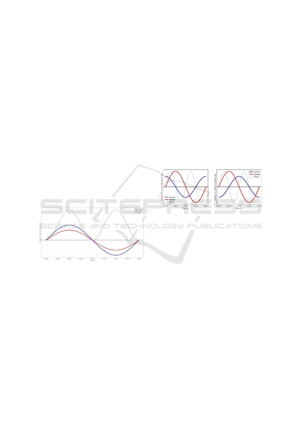
As a result, in a resistive circuit, the current also

oscillates at the same frequency, because the resis-

tive load current is directly proportional to the applied

voltage. Figure 1 shows the correlation between volt-

age (red), current (blue) and power (green). Instanta-

neous power (since it is the product of the voltage and

current) oscillates at twice the voltage frequency, but

unlike the other two, in such a purely resistive cur-

rent the power never drops to negative. This part of

the power ﬂow (or its averaged value over one cycle

of the AC circuit), is known as real power or active

power and it always ﬂows from the direction of the

source to the load while transferring the net energy

(Zhou et al., 2018; Mukherjee et al., 2018; Mbinkar

et al., 2022).

Figure 1: Voltage, current and power in a purely resisive AC

circuit.

Distribution and transmission systems are pro-

posed to transfer active power from power stations

to energy consumers. The number of loads requires

for operation not only the active power, but reactive

power, as well. For example, AC motors require mag-

netic ﬁelds, which are generated by inductors that

consume a so-called reactive power. Moreover, all

components in inductive reactance distribution and

transmission systems (cables, transformers) require

reactive power.

Induction elements such as electric motors, trans-

formers or induction cookers store energy in their

magnetic ﬁeld, which direction is opposite to the

change in voltage. Thus, as the supply voltage rises,

the net voltage on the inductor rises more slowly due

to the reverse voltage, which is induced by the induc-

tor. This causes the current lagging behind the voltage

since the current is proportional to the voltage in the

circuit. In a purely inductive circuit, the current lags

90 degrees behind the voltage.

Capacitive elements e.g., capacitors, overhead

power wires, electrical cables, or ﬂuorescent lamps

store energy in their electric ﬁeld. The behavior of

the capacitive circuit is best best seen on the exam-

ple of the capacitor. The pressure difference across

the plates of a capacitor is the result of the accumula-

tion of electrons on one plate and lack of electron on

the other one. When the plates are uncharged, the in-

creasing voltage from the supply sends the maximum

current in the circuit to be stored on the plates until

they become full of charge and no more charge is be-

ing added. At this point the voltage reaches its peak

and the current is zero. In a pure capacitive circuit, the

current leads the voltage by 90 degrees (Zhou et al.,

2018; Mukherjee et al., 2018; Mbinkar et al., 2022).

Figure 2: Voltage, current and power in an AC circuit where

the current lags (left) and leads (right) the voltage.

Unlike in a resistive circuit, in a capacitive or in-

ductive circuit the instantaneous power oscillates be-

tween a negative and a positive maximum, averaging

zero during one network cycle, as it is seen in Fig-

ure 2. The seemingly negative part of the power is

being returned to the source in each cycle and it is

called reactive power. No net energy can be transmit-

ted using reactive power.

The real networks consist of both resistive and re-

active loads, which form together the complex (ap-

parent) power expressed as volt-amperes (VA). The

ratio of the active power to the apparent power de-

ﬁnes the power factor of the circuit that describes the

amount of the real power transmitted to the load along

the transmission line to the total apparent power ﬂow-

ing in the line. The apparent power is the vector sum

of active and reactive power, which is visualised in

Figure 3 as the so-called power triangle (Maitre and

Glon, 2015; Zhao et al., 2005).

The power factor might also be computed as the

cosine of the angle φ, called the phase angle, by which

the current waveform leads or lags the voltage wave-

form. Both methods afﬁrm, that the potential values

Automatic Reactive Power Classiﬁcation Based on Selected Machine Learning Methods

101

Figure 3: The power triangle of the real power, reactive

power and apparent power.

of the power factor are within the interval (0,1): the

closer the power factor is to 1, the more efﬁcient the

circuit, and vice versa.

3 METHODS

In this section, we describe our dataset, characteristics

of attributes, training set and classiﬁcation methods

used for our analysis.

Our core focus is to advance research in the ﬁeld

of binary classiﬁcation of electricity consumers based

on their power factor. We used a period of three weeks

as the observation period and one week as the result-

ing period. In particular, we explore if the power fac-

tor will be lower than 0.98 at least one day in the fol-

lowing week based on data about the power factor of

the previous three weeks. Our aim is to ﬁnd the most

efﬁcient algorithm and the most appropriate hyperpa-

rameter values for the chosen problem.

3.1 Dataset

Multifamily residential dataset of electricity (Mein-

renken et al., 2020) includes the annual electricity

use of 390 apartments located in the Northeastern

United States. These apartments are organized into

26 groups of 15 apartments each by their total elec-

tricity consumption in 2019. The apartments differ

in the construction year (constructed before 1940, be-

tween 1940-1980, or constructed after 1980). More-

over, they use different cooling system or heating sys-

tem (stem water, hot water, packaged terminal air con-

ditioning units).

Time stamp, instantaneous real and reactive

power, and cumulative electricity consumed are in-

cluded for each of the 26 apartments groups. Data

at 10-second or 15-minutes time resolution are avail-

able, which corresponds to 3,153,600 and 35,040

number of rows, respectively.

3.2 Extracted Attributes and Training

Set

For our analysis, we use the data at 15 minutes time

resolution of instantaneous real power and reactive

power.

Let O = {o

, o

, . . . , o

} be the set of 26 groups

of apartments and T = {t

, t

, . . . , t

35040

} be the index

of timestamp in 2019 at 15 minutes time resolution.

Thus, the value P(o, t) corresponds to the instanta-

neous real power of the group o ∈ O in the time t ∈ T .

Analogously, the value Q(o, t) corresponds to the in-

stantaneous reactive power of the group o ∈ O in the

time t ∈ T . The unit of active and reactive power is

kW and kVar, respectively.

Since the phase angle and power factor are not in-

cluded in the original multifamily residential dataset

of electricity, we need to compute the phase angle as

the binary relation

φ(o, t) = arctan

P(o, t)

Q(o, t)

and power factor as the binary relation

F(o, t) = cos(φ(o, t))

for each o ∈ O and t ∈ T , i.e. at 15 minutes time

resolution for each 26 groups of apartments.

Note that F(o, t) ∈ [−1;1] for each o ∈ O and

t ∈ T . If power factor is equal to 0 (i.e., F(o, t) = 0 for

some o ∈ O and t ∈ T ), the energy ﬂow is entirely re-

active and the energy in the load returns to the source

on each cycle. If the power factor is 1 (i.e., F(o, t) = 1

for some o ∈ O and t ∈ T ), all the energy supplied by

the source is consumed by the load.

In order to construct the training set, we create

a period of 3 weeks as the observation period and 1

week as the result period. In particular, our models are

built by data from the observation period of 3 weeks

to classify if the power factor will be lower than 0.98

at least one day in the following week. Thus, our tar-

get attribute has two categories.

Regarding the input attributes, we take 6 origi-

nal attributes from the original multifamily residential

dataset of electricity (number of bedrooms, number

of all rooms, apartment area and their standard de-

viations). However, we constructed additional 28 at-

tributes from the binary relation F(o, t) for each o ∈ O

and t ∈ T . The extracted attributes are described in

Table 1. Low excess of reactive power means that

power factor F(o, t) will be lower than 0.98 at least in

one day of the week. Medium excess means that the

power factor F(o, t) will be lower than 0.98 at least

in two days of the week. High excess means that the

power factor F(o, t) will be lower than 0.98 at least in

three days of the week.

ICAART 2023 - 15th International Conference on Agents and Artiﬁcial Intelligence

102

Table 1: The extracted attributes and their tpyes.

Characteristics Period Type

Month nominal

Low excess 1.-3. week binary

Low excess 1. week binary

Low excess 2. week binary

Low excess 3. week binary

Medium excess 1. week binary

Medium excess 2. week binary

Medium excess 3. week binary

High excess 1. week binary

High excess 2. week binary

High excess 3. week binary

Proportion of excess 1. week [0,1]

Proportion of excess 2. week [0,1]

Proportion of excess 3. week [0,1]

Average of F 1.-3. week [0,1]

Standard deviation of F 1.-3. week [0,1]

Minimum of F 1.-3. week [0,1]

Maximum of F 1.-3. week [0,1]

25th percentile of F 1.-3. week [0,1]

75th percentile of F 1.-3. week [0,1]

Median of F 1.-3. week [0,1]

Average of F 3. week [0,1]

Standard deviation of F 3. week [0,1]

Minimum of F 3. week [0,1]

Maximum of F 3. week [0,1]

25th percentile of F 3. week [0,1]

75th percentile of F 3. week [0,1]

Median of F 3. week [0,1]

3.3 Learning Algorithms

To solve our binary classiﬁcation task, we use the fol-

lowing learning algorithms (methods):

• naive classiﬁcation by using the high excess in last

three weeks (which served as a baseline),

• Gaussian naive Bayes,

• k-nearest neighbors classiﬁer,

• support vector classiﬁer,

• deep feedforward neural network,

• logistic regression,

• decision trees,

• AdaBoost classiﬁer

• GradientBoosting classiﬁer,

• random forests,

• balanced random forests classiﬁer,

The main motivation for using these algorithms

is to compare the performance of various popular

machine learning methods on the selected data set.

For hyper-parameter optimization, we used the grid

search method, which is thoroughly described for ex-

ample in (Mantovani et al., 2016; Feurer and Hutter,

2019; Wu et al., 2019; Yang and Shami, 2020).

As our baseline method, we use the high excess

of power factor of the last 3 weeks of the observation

period. The baseline method is stronger than random

assignment, since a high proportion of power factor

excess in the actual period can be a strong indicator of

a high proportion of power factor excess in the future.

Naive Bayes Method: is based on Bayes’ theo-

rem with the “naive” assumption of conditional in-

dependence between each pair of attributes given the

value of the target attribute (Rish, 2001; Chen et al.,

2020). We apply the Gaussian algorithm, since the

likelihood of the features is assumed to be Gaussian.

Nearest Neighbor Methods: are based on ﬁnd-

ing a particular number of training examples closest

in distance to the new example, and classify the label

from these. The number of examples can be given by

a user by parameter or can vary on the local density of

points (Jiang et al., 2007; Gou et al., 2019). We use

parameters k = 6 for number of neighbors, distance

metric and p = 3 for the Minkowski metric.

Support Vector Classiﬁcation: methods use a

subset of training points for the decision function (in

the role of support vector) and they provide diverse

options for building the decision function (Christiani

and Shawe-Taylor, 2000). These methods were pro-

posed at AT&T Bell in New Jersey around 1995 and

they were used to recognize handwritten digits on

postal items. We use the linear kernel with regular-

ization parameter of value 1.

Feedforward Neural Network: is a non-linear

function approximator for classiﬁcation, which con-

tains the input layer, the output layer, and there can

be one or more non-linear layers, called hidden lay-

ers, between input and output layers (Glorot and Ben-

gio, 2010). We use the multilayer perceptron with

one hidden layer of 300 neurons, relu activation func-

tion, adam solver for weight optimization, and con-

stant learning rate.

Logistic Regression: is a linear model for classi-

ﬁcation which describes the probabilities of the possi-

ble outputs of a single example. The probabilities are

modeled by applying a logistic function (Kleinbaum

et al., 2002). We use maximum number of 500 iter-

ations taken for the solvers to converge, both L1 and

L2 penalty terms and the elastic-net mixing parameter

with L1 ratio of 0.7.

A decision tree method builds in the data a hier-

archical structure, implementing divide-and-conquer

strategy. It is an efﬁcient method which can be used

Automatic Reactive Power Classiﬁcation Based on Selected Machine Learning Methods

103

both for classiﬁcation (just splitting the data into some

categories) and regression (predicting also the typical

values in different categories (Breiman, 2001; Alpay-

din, 2010). Decision trees are designed for dependent

variables that take a ﬁnite number of unordered val-

ues, with prediction error measured in terms of mis-

classiﬁcation cost. Decision trees are constructed us-

ing a recursive partitioning algorithm. This algorithm

builds a tree by recursively splitting the training sam-

ple into smaller subsets. The algorithm has three main

components:

• a way to select a splitting rule,

• a rule to determine when a tree node is terminal

(termination criterion),

• a rule for assigning a value to each terminal node.

For decision tree, we use gini index to measure the

quality of a split, the maximum depth of the tree of 5,

and the minimum 4 of samples required to be at a leaf

node.

AdaBoost: (abbreviation from Adaptive Boost-

ing) classiﬁcation is an ensemble classiﬁcation

method which is based on an iterative approach to

learn from the mistakes of weak classiﬁers. It starts

by training a classiﬁer on the original data. Thus,

the additional copies of the classiﬁer are constructed

on the same dataset. However, the weights of incor-

rectly classiﬁed examples are modiﬁed (Freund and

Schapire, 1997). We use decision tree classiﬁer as the

base estimator for AdaBoost classiﬁcation. We use

the maximum number of 1000 estimators at which

boosting is terminated.

Gradient Boosting: classiﬁer is an ensemble

classiﬁcation method which generalizes the other

boosting methods by allowing optimization of an ar-

bitrary differentiable loss function (Friedman, 2001).

We use decision tree classiﬁer as the base estimator

for gradient boosting classiﬁcation. We use the num-

ber of 1000 boosting stages to perform.

Random Forests: are a combination of tree clas-

siﬁers such that each tree depends on the values of

a random vector sampled independently and with the

same distribution for all trees in the forest (Breiman,

2001). The principle is averaging classiﬁcations over

a large number of trees learned on randomly chosen

subsets of features (predictors). We use 2000 decision

trees in the random forest, the gini index to measure

the quality of a split, the maximum depth of 5, and 5

features to consider if looking for the best split.

Balanced Random Forest: classiﬁer is the exten-

sion of random forests since the classiﬁcation tasks

are often imbalanced which means that at least one

of the categories comprises only a small minority of

the data. This issue can be solved by adding the

class weights to the random forest classiﬁer. Thus,

it penalizes misclassifying the minority category. On

the other hand, down-sampling the majority class and

growing each tree on a more balanced data set can be

applied (Chen et al., 2004). We use 2000 decision

trees in the random forest, the gini index to measure

the quality of a split, the maximum depth 5 of the tree,

and 5 features to consider if looking for the best split.

3.4 Comparing Classiﬁcation Methods

For the evaluation of algorithms, we used an exten-

sion of 5-fold cross validation which returns stratiﬁed

folds. It means that the folds are constructed by pre-

serving the percentage of samples for each class. In

our experiments, we computed the accuracy, F1 score,

and F2 score for each of the described methods.

Dietterich described the principles of ﬁve statisti-

cal tests (McNemar’s test, a test for the difference of

two proportions, the resampled paired t test, the k-fold

cross-validated paired t test, and the 5 × 2 cv paired

t test) for deciding if one learning algorithm (super-

vised classiﬁcation method) outperforms another (Di-

etterich, 1998; Raschka, 2018). He argued that the

5 × 2 cross-validation test is mostly recommended

since it is slightly more powerful and it measures vari-

ation due to the selection of the training set. By this

recommended test, we performed ﬁve duplicates of

2-fold cross-validation for each pair of our methods

(learning algorithm). In each duplicate, data from our

paper are randomly partitioned into two equal sized

sets, and each method (learning algorithm) is trained

on each set and tested on the other set.

4 RESULTS

In this subsection we present our results, including

the statistical tests for comparing supervised classiﬁ-

cation learning algorithms.

The overall results are described in Table 2. We

present the accuracy, F1 score, and F2 score for each

of the described methods.

In Figure 4, we present the comparison of F1

scores of 10 learning algorithms on folds of 5-fold

cross validation. The abbreviations of the algorithms

in diagram corresponds to the titles of methods in-

troduced in Table 2. We found that the smallest dif-

ference between F1 scores of folds was observed by

gradient boosting classiﬁer.

The results of the 5 × 2 cv paired t test (described

in Subsection 3.4) are shown in Table 3. We found

that there is a statistically signiﬁcant difference be-

tween mean F1 score of random forest algorithm

ICAART 2023 - 15th International Conference on Agents and Artiﬁcial Intelligence

104

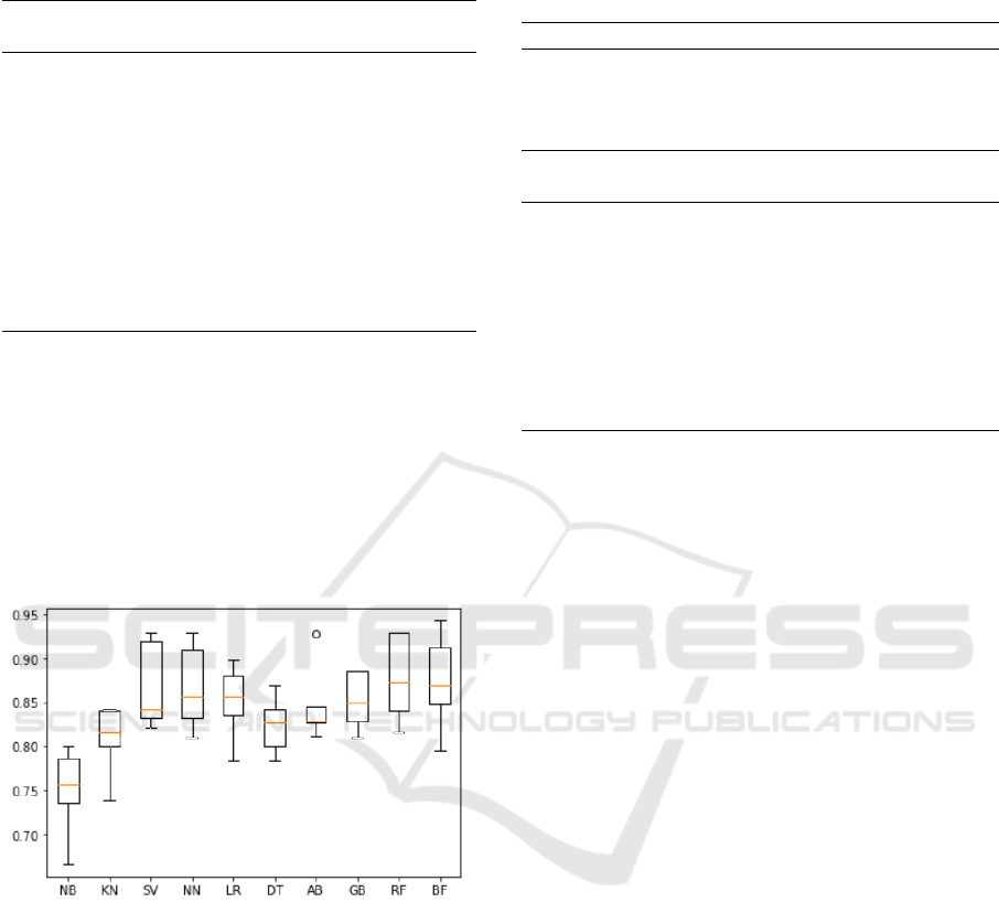
Table 2: The overall results on binary classiﬁcation task.

Algorithm Accu- F1 F2

racy score score

Baseline 0.71 0.668 0.569

Naive Bayes (NB) 0.76 0.750 0.673

Nearest neighbors (NN) 0.78 0.808 0.818

Support vector (SV) 0.85 0.869 0.883

Neural network (NN) 0.85 0.868 0.880

Logistic regression (LR) 0.83 0.851 0.849

Decision tree (DT) 0.79 0.824 0.835

AdaBoost (AB) 0.83 0.848 0.845

Gradient boost (GB) 0.83 0.852 0.852

Random forest (RF) 0.86 0.877 0.880

Balanced forest (BF) 0.86 0.873 0.858

and naive Bayes algorithm, or between random for-

est algorithm and nearest neighbors algorithm. There

is also a statistically signiﬁcant difference between

mean F1 score of balanced forest algorithm and naive

Bayes algorithm, or between balanced forest algo-

rithm and nearest neighbors algorithm. Surprisingly,

if the 5 × 2 cv paired t test is applied between neural

network algorithm and logistic regression, difference

between mean performance is probably real.

Figure 4: Comparison of F1 scores on folds.

5 DISCUSSION

Multifamily residential dataset of electricity (Mein-

renken et al., 2020) provides the unique source of 12-

month duration data of apartment electricity use in

the multifamily area. This type of data is valuable

since residential building sector responds for over

30% of the energy consumption worldwide (Mein-

renken et al., 2020; Li et al., 2021a).

We have not found a similar study of power factor

classiﬁcation in the literature for this particular data

set. However, we present the other interesting tasks

solved on these data set in Discussion, which have

Table 3: Comparison of learning algorithms by 5 × 2 cv

paired t test.

NB KN SV NN LR

NB – 0.252 0.012

∗

0.042

∗

0.299

KN – 0.036

∗

0.025

∗

0.055

SV – 0.941 0.141

NN – 0.021

∗

DT AB GB RF BF

NB 0.370 0.038

∗

0.035

∗

0.011

∗

0.006

∗

KN 0.114 0.023

∗

0.024

∗

0.024

∗

0.027

∗

SV 0.648 0.908 0.713 0.268 0.178

NN 0.688 0.882 0.847 0.480 0.703

LR 0.885 0.229 0.254 0.056 0.111

DT – 0.680 0.434 0.439 0.533

AB – 0.650 0.364 0.234

GB – 0.619 0.925

RF – 0.687

∗

statistically signiﬁcant difference on level 0.05

been published by researchers recently. They mainly

focus on the analysis of the active power and they do

not consider the reactive power, as it is described in

our paper. Thus, we hope that our paper can provide

the added value in this interesting issue of electricity

consumption.

Regarding the scientiﬁc papers related to this orig-

inal dataset, researchers (Li et al., 2021b) explored

the effects of outdoor temperature and COVID-19 re-

lated stay-at-home restrictions in residential electric-

ity usage. They applied the set of regression meth-

ods to predict the average consumption over the spe-

ciﬁc time windows on weekdays. Moreover, they ap-

plied Monte Carlo methods to predict the effects of

COVID-19 related stay-at-home restrictions. These

types of results can help for managers to improve the

balance of demand and supply in future. The results

of data analysis can help citizens to load-shift part of

their electricity usage, e.g. from day time to night.

In this way, the feedback to residents about the

usage of electricity can help to immediately reduce

demand, however an effect of boomerang can appear,

as well (Meinrenken et al., 2021; Asensio and Del-

mas, 2015). The results of feedback effectiveness

study have shown the average observed reduction of

electricity usage of approximately 11% versus con-

trol group with no feedback. The text messages of

feedback for residents were generated by the meth-

ods of natural language processing (Meinrenken et al.,

2021).

Another study (Cen et al., 2022) analyzed mul-

tifamily residential dataset of electricity (Meinrenken

et al., 2020) from the clustering point of view. The au-

Automatic Reactive Power Classiﬁcation Based on Selected Machine Learning Methods

105

thors presented four phases of their analysis – cleans-

ing of data, extraction of features by multilevel dis-

crete wavelet transformation, reduction of dimension-

ality by Pearson correlation coefﬁcients and by prin-

cipal component analysis, and the phase of clustering

by k-means, fuzzy c-means, and hierarchical cluster-

ing. They found the representative electricity load

patterns in three clusters – group of low load con-

sumption, medium load consumption, or high load

consumption including instability group. These pat-

terns can be used to maintain the stability of power

system or to design the optimal strategies for energy

consumption.

We emphasize that other related datasets are avail-

able, as well. For example, a synthetic building oper-

ation dataset (Li et al., 2021a) contains electric loads,

end-use energy consumptions, or historical weather

data. It can be used to construct novel datasets with

various conditions on weather, behavior of residents,

or type of building.

Recently, a home energy management device was

installed in the apartment house with 365 ﬂats in

Tokyo to measure the energy consumption data, and

gas use (Yoshida et al., 2021). They argued that im-

plementation of practises for energy saving of resi-

dents is becoming an important challenge and they

proposed the optimal energy-saving behaviours.

Multifamily residential dataset of electricity

(Meinrenken et al., 2020) contains both instantaneous

active and reactive power. We would like to put em-

phasis that our approach provides the additional re-

sults to the mentioned researchers since we did not

found the papers which analyze the reactive power for

this dataset. However, the reactive power allows us to

analyze the phase angle and the power factor of the

apartments since it can help to reduce energy waste

in homes and the built environment. Moreover, the

optimization of reactive power and power factor can

be fruitful in the process of building a smart environ-

ment, as well.

6 CONCLUSIONS

In this paper, we presented an automatic reactive

power classiﬁcation based on selected machine learn-

ing methods. We predicted an excess of reactive

power in the particular buildings from multifamily

residential electricity dataset. Moreover, we pre-

sented the 5 × 2 cross validation test of the several

machined learning methods. Finally, we discussed the

added value of our paper in comparison with other re-

lated studies.

In our region, the energy company East Slovakia

Distribution distributes the electricity via its own dis-

tribution system to the end customer. Regarding our

cooperation with this company, we have an access

to real data of reactive power of 70,000 households,

30,000 companies and 5,000 transformer stations. In

our future work, we plan to analyze these data of cus-

tomers regarding the possibility to reduce the reactive

power in the electricity system.

ACKNOWLEDGEMENTS

This work was supported by the Scientiﬁc Grant

Agency of the Ministry of Education, Science, Re-

search and Sport of the Slovak Republic under

contract VEGA 1/0177/21 Descriptive and com-

putational complexity of automata and algorithms

(G. Semani

sin, V. Prista

s) and under contract

VEGA 1/0645/22 Proposal of novel methods in the

ﬁeld of Formal Concept Analysis and their applica-

tion (L. Antoni). We would like to kindly thank the

employees of the Data Collection and Management

Department in energy company East Slovakia Distri-

bution, Jozef Dudiak and J

an Pirigyi, for motivation

and discussions on reactive power, as well as for the

real data regarding our future work. We would like to

thank Professor Peter Koll

ar, the head of Institute of

Physics at Faculty of Science at Pavol Jozef

Saf

arik

university, for his fruitful remarks and comments on

reactive power principles.

REFERENCES

Alahmad, M., Hasna, H., and Sordiashie, E. (2011).

Non-intrusive electrical load monitoring and proﬁling

methods for applications in energy management sys-

tems. In IEEE long island systems, applications and

technology conference, pages 1–6. IEEE.

Alpaydin, E. (2010). Introduction to Machine Learning.

MIT Press.

Anaya, K. L. and Pollitt, M. G. (2020). Reactive power pro-

curement: A review of current trends. Applied Energy,

270:114939.

Asensio, O. and Delmas, M. (2015). Nonprice incentives

and energy conservation. Proceedings of the National

Academy of Sciences, 112(6):E510–515.

Breiman, L. (2001). Random forests. Machine learning,

45(1):5–32.

Cen, S., Yoo, J. H., and Lim, C. G. (2022). Electric-

ity pattern analysis by clustering domestic load pro-

ﬁles using discrete wavelet transform. Scientiﬁc data,

15(4):1350.

Chen, C., Liaw, A., and Breiman, L. (2004). Using ran-

dom forest to learn imbalanced data. University of

California, Berkeley.

ICAART 2023 - 15th International Conference on Agents and Artiﬁcial Intelligence

106

Chen, S., Webb, G. I., Liu, L., and Ma, X. (2020). A novel

selective na

ıve bayes algorithm. Knowledge-Based

Systems, 192:106361.

Christiani, N. and Shawe-Taylor, J. (2000). An introduc-

tion to support vector machines. Cambridge Univer-

sity Press.

Dietterich, T. G. (1998). Approximate statistical tests

for comparing supervised classiﬁcation learning algo-

rithms. Neural computation, 10(7):1895–1923.

Dixon, J., Moran, L., Rodriguez, J., and Domke, R. (2005).

Reactive power compensation technologies: State-of-

the-art review. Proceedings of the IEEE, 93(12):2144–

2164.

Feurer, M. and Hutter, F. (2019). Hyperparameter optimiza-

tion. In Automated machine learning, pages 3–33.

Springer, Cham.

Freund, Y. and Schapire, R. E. (1997). A decision-theoretic

generalization of on-line learning and an application

to boosting. Journal of computer and system sciences,

55(1):119–139.

Friedman, J. (2001). Greedy function approximation: A

gradient boosting machine. The Annals of Statistics,

29(5).

Glorot, X. and Bengio, Y. (2010). Understanding the dif-

ﬁculty of training deep feedforward neural networks.

In International Conference on Artiﬁcial Intelligence

and Statistics.

Gou, J., Ma, H., Ou, W., Zeng, S., Rao, Y., and Yang, H.

(2019). A generalized mean distance-based k-nearest

neighbor classiﬁer. Expert Systems with Applications,

115:356–372.

Jiang, L., Cai, Z., Wang, D., and Jiang, S. (2007). Survey

of improving k-nearest-neighbor for classiﬁcation. In

Fourth international conference on fuzzy systems and

knowledge discovery (FSKD 2007), pages 679–683.

Kleinbaum, D. G., Dietz, K., Gail, M., Klein, M., and Klein,

M. (2002). Logistic regression. New York: Springer-

Verlag.

Li, H., Wang, Z., and Hong, T. (2021a). A synthetic build-

ing operation dataset. Scientiﬁc data, 8(1):1–13.

Li, L., Meinrenken, C. J., Modi, V., and Culligan, P. J.

(2021b). Impacts of covid-19 related stay-at-home

restrictions on residential electricity use and implica-

tions for future grid stability. Energy and Buildings,

251:111330.

Maitre, J. and Glon, G. (2015). Efﬁcient appliances recog-

nition in smart homes based on active and reactive

power, fast fourier transform and decision trees. In

Workshops at the Twenty-Ninth AAAI Conference on

Artiﬁcial Intelligence. SCITEPRESS.

Mantovani, R. G., Horv

ath, T., Cerri, R., Vanschoren, J.,

and de Carvalho, A. C. (2016). Hyper-parameter

tuning of a decision tree induction algorithm. In

2016 5th Brazilian Conference on Intelligent Systems

(BRACIS), pages 37–42. IEEE.

Mbinkar, E. N., Asoh, D. A., and Kujabi, S. (2022). Mi-

crocontroller control of reactive power compensation

for growing industrial loads. Energy and Power Engi-

neering, 14(9):460–476.

Meinrenken, C. J., Abrol, S., Gite, G. B., Hidey, C.,

McKeown, K., Mehmani, A., Modi, V., Turcan, E.,

Xie, W., and Culligan, P. J. (2021). Residential

electricity conservation in response to auto-generated,

multi-featured, personalized eco-feedback designed

for large scale applications with utilities. Energy and

Buildings, 232:110652.

Meinrenken, C. J., Rauschkolb, N., Abrol, S., Chakrabarty,

T., Decalf, V. C., Hidey, C., McKeown, K., Mehmani,

A., Modi, V., and Culligan, P. J. (2020). Mfred, 10

second interval real and reactive power for groups of

390 us apartments of varying size and vintage. Scien-

tiﬁc Data, 7:375.

Mukherjee, S., Ganguly, A., Paul, A. K., and Datta, A. K.

(2018). Load ﬂow analysis and reactive power com-

pensation. In 2018 International Conference on

Computing, Power and Communication Technologies

(GUCON), pages 207–211. IEEE.

Raschka, S. (2018). Mlxtend: Providing machine learning

and data science utilities and extensions to python’s

scientiﬁc computing stack. The Journal of Open

Source Software, 3(24).

Rish, I. (2001). An empirical study of the naive bayes clas-

siﬁer. IJCAI 2001 workshop on empirical methods in

artiﬁcial intelligence, 3(22):41–46.

Sarkar, M. N. I., Meegahapola, L. G., and Datta, M. (2018).

Reactive power management in renewable rich power

grids: A review of grid-codes, renewable generators,

support devices, control strategies and optimization

algorithms. IEEE Access, 6:41458–41489.

ellez, A. A., L

opez, G., Isaac, I., and Gonz

alez, J. W.

(2018). Optimal reactive power compensation in elec-

trical distribution systems with distributed resources.

review. Heliyon, 4(8):e00746.

Vishnu, M. and Kumar, S. (2020). An improved solution

for reactive power dispatch problem using diversity-

enhanced particle swarm optimization. Energies,

13(11):2862.

Wu, J., Chen, X. Y., Zhang, H., Xiong, L. D., Lei, H., and

Deng, S. H. (2019). Hyperparameter optimization for

machine learning models based on bayesian optimiza-

tion. Journal of Electronic Science and Technology,

17(1):26–40.

Yang, L. and Shami, A. (2020). On hyperparameter opti-

mization of machine learning algorithms: Theory and

practice. Neurocomputing, 415:295–316.

Yoshida, K., Rijal, H. B., Bogaki, K., Mikami, A., and

Abe, H. (2021). Field study on energy-saving be-

haviour and patterns of air-conditioning use in a con-

dominium. Energies, 14(24):8572.

Zhao, Y., Irving, M. R., and Song, Y. (2005). A cost alloca-

tion and pricing method for reactive power service in

the new deregulated electricity market environment.

In 2005 IEEE/PES Transmission & Distribution Con-

ference & Exposition: Asia and Paciﬁc, pages 1–6.

IEEE.

Zhou, X., Wei, K., Ma, Y., and Gao, Z. (2018). A re-

view of reactive power compensation devices. In 2018

IEEE International Conference on Mechatronics and

Automation (ICMA), pages 2020–2024. IEEE.

Automatic Reactive Power Classiﬁcation Based on Selected Machine Learning Methods

107