A Comparison of Several Speed Computation Methods for the Safe

Shortest Path Problem

Aur

elien Mombelli, Alain Quilliot and Mourad Baiou

LIMOS, UCA, 1 Rue de la Chebarde, 63170 Aubi

ere, France

Keywords:

Dynamic Programming, Risk Aware, Time-Dependant, Reinforcement Learning.

Abstract:

This paper is based on (Mombelli et al., 2022). In their article, they dealt with a ﬂeet of autonomous vehicles

which is required to perform internal logistics tasks in some protected areas. This ﬂeet is supposed to be

ruled by a hierarchical supervision architecture which, at the top level, distributes and schedules Pick up and

Delivery tasks, and, at the lowest level, ensures safety at the crossroads and controls the trajectories. They

presented the problem of ﬁnding a shortest path under risk constraints and proposed a way to compute speed

functions along the path. In this paper, we present some theoretical results and focus on the ﬁxed path problem.

We propose several new ways of computing speed functions including a couple with reinforcement learning.

1 INTRODUCTION

While human drivers are capable of local risk avoid-

ance, autonomous vehicles (AV) do not have such in-

trinsic capabilities and risk aware algorithms are ab-

solutely necessary.

Monitoring a ﬂeet involving AVs usually relies on

hierarchical supervision. The trend is to use three

levels. At the low level, or embedded level, robotic-

related problems are tackled for speciﬁc AVs like con-

trolling trajectories in real-time and adapting them

to the possible presence of obstacles, see (Mart

ınez-

Barber

a and Herrero-P

erez, 2010). At the middle

level, or local level, local supervisors manage prior-

ities among AVs and resolve conﬂicts in a restricted

area (Chen and Englund, 2016; Philippe et al., 2019)

who worked on crossroad strategies. Then, at the top

level, or global level, global supervisors assign tasks

to the ﬂeet and schedule paths. This level must take

lower levels into account to compute its solution. See

(Koes et al., 2005; Vis, 2006; Le-Anh and De Koster,

2006) for example or (Wurman et al., 2008) who com-

pute the shortest path thanks to the A* algorithm but

assign each task to the ﬂeet of AVs using a multi-agent

artiﬁcial intelligence to avoid most conﬂicts in arcs.

This study puts the focus on the global level: rout-

ing and giving instructions to an AV in a ﬂeet. An AV,

idle until now, is chosen to carry out a new task. Since

a vehicle is moving from some origin to some desti-

nation, performing some loading or unloading trans-

action and keeping on. But some speciﬁc features im-

pose new challenges:

• The time horizon for AVs is usually short and

decisions have to be taken online, which means

that decision processes must take into account

the communication infrastructure, see (Vivaldini

et al., 2013), and the way the global supervisor

can be provided, at any time, with a representa-

tion of the current state of the system and its short

term evolution;

• As soon as AVs are involved, safety is at stake

(see (Pimenta et al., 2017)). The global supervi-

sor must compute and schedule routes in such a

way that not only tasks are going to be efﬁciently

performed, but also that local and embedded su-

pervisors will perform their job safely.

To compute a safe shortest path, (Ryan et al., 2020)

used, a weighted sum of time and risks in Munster’s

roads in Ireland using an A* algorithm. In their case,

the risk is a measure of dangerous steering or brak-

ing events on roads. But these techniques mostly can-

not be applied here because the risk, in our case, is

time-dependent. Here, the risk will not be a mea-

sure of dangerous events on the roads of a city but

the expected repair costs in a destructive accident sce-

nario, should it happens. To compute such expecta-

tion, planning of risks is to be computed from the al-

ready working ﬂeet because the path they will follow

and their speed functions are known. A risk planning

procedure is then used to transform previous informa-

tion into risk functions over time that is necessary to

Mombelli, A., Quilliot, A. and Baiou, M.

A Comparison of Several Speed Computation Methods for the Safe Shortest Path Problem.

DOI: 10.5220/0011618600003396

In Proceedings of the 12th International Conference on Operations Research and Enterprise Systems (ICORES 2023), pages 15-26

ISBN: 978-989-758-627-9; ISSN: 2184-4372

 2023 by SCITEPRESS – Science and Technology Publications, Lda. Under CC license (CC BY-NC-ND 4.0)

compute the expected repair costs for the AV.

In an article presented at the ICORES conference

in 2022, (Mombelli et al., 2022) presented the prob-

lem of ﬁnding a shortest path under risk constraints

and proposed a way to compute speed functions along

the path. In this contribution, we will present new ad-

vances related to:

• the comprehension of the way risk functions may

be deﬁned and computed

• the complexity of the global problem

• the different ways decisions may be designed and

induce transitions

• the way statistical learning may be involved in or-

der to ﬁlter both decisions and states

First, a precise description of the global problem is

presented with structural results. Then, the prob-

lem with ﬁxed path where only the speed functions

are unknown is tackled and it’s complexity is dis-

cussed. In the fourth section, the ﬁxed path prob-

lem is approached with dynamic programming with

several speed generation methods followed by, in the

ﬁfth section, ﬁltering and learning processes. Lastly,

numerical experiments are presented with a conclu-

sion.

2 RISK INDUCED BY THE

ACTIVITY OF AN AV FLEET

In this section, the problem we already talked about in

the previous paper is described together with the spe-

ciﬁc problem on a ﬁxed path. Then, some structural

results of the solution will be presented leading to a

reformulation of our problem. Lastly, the complexity

of the problem is tackled.

2.1 Measuring the Risk

A warehouse is represented as a planar connected

graph G = (N,A) where the set of nodes N represents

crossroads and the set of arcs A represents aisles. For

any arc a ∈ A, L

represents the minimal travel time

for an AV to go through aisle a. Moreover, two aisles

may be the same length but one may stock fragile ob-

jects so that vehicles have to slow down.

Also, risk functions Π

: t 7→ Π

(t), generated

from activities of aisle a, are computed using the risk

planning procedure on experimentation in a real ware-

house that we are provided with. It is important to

note that the risk is not continuous. Indeed, there is,

in an aisle, a ﬁnite number of possible conﬁgurations:

empty, two vehicles in opposite directions, etc. (see

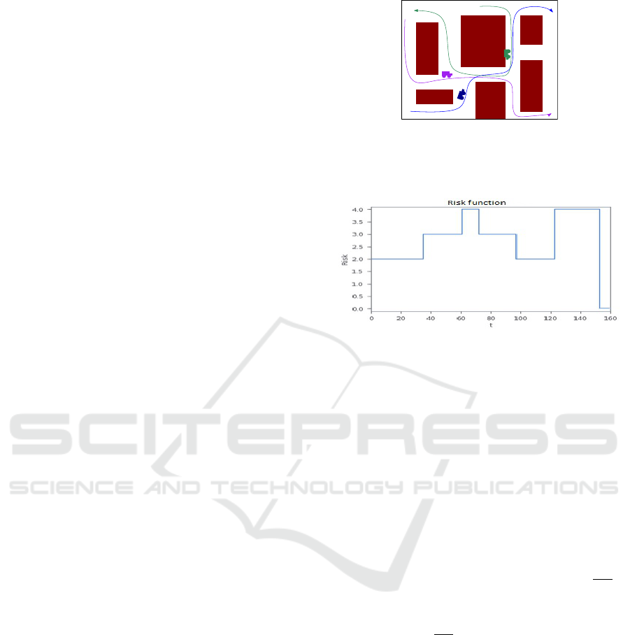
Figure 1: At time t, 3 aisles have 1 vehicle each. At the

next time , Blue and Purple join in the same aisle. One time

after, all 3 vehicles join, generating high risks in this aisle

(ﬁgure from (Mombelli et al., 2022)).

Figure 2: Risk function of an aisle (ﬁgure from (Mombelli

et al., 2022)).

Figure 1). Each conﬁguration is, then, associated with

an expected cost of repairs in the event of accidents.

Therefore, they are staircase functions evaluated in a

currency (euro, dollars, etc.). Figure 2 shows an ex-

ample of a risk function of an aisle.

From a risk function, we can have an estimation of

the risk an AV takes in an aisle a between two times

and t

with v : t 7→ v(t) as its speed function with

Equation 1.

risk(t

,v) = H(v)

(t)dt (1)

We impose function H to be such that H(v) ≪

max

order to express the fact that a decrease of the speed

implies a decrease of the risk. In further sections, H

is set to H : v 7→



max



Remark 1. Speed Normalization: We only care here

about traversal times of arcs e ∈ A, and not about

their true length, in the geometric sense. So we sup-

pose, without loss of generality that, for any arc e,

max

= 1. Therefore we deal with reduced speed val-

ues v ∈ [0,1] and L

means the minimal traversal time

for arc e.

2.2 Discussion About Risk Functions

We are going to discuss here the way functions Π

come from and how they can be derived from obser-

vations in a real example. As a matter of fact, the key

issue is about the way the risk related to the activity

ICORES 2023 - 12th International Conference on Operations Research and Enterprise Systems

of a ﬂeet of AVs inside a transit network G = (N,A)

may be deﬁned.

In any case, the risk should be deﬁned here as re-

lated to the expected damage

[t,t+dt]

(s).ds which

is induced, on a given arc e and during a time in-

terval [t,t + dt], by the activity of the ﬂeet along arc

e. It comes that the issue for us is to determine risk

functions t 7→ Π

(t),e ∈ A. We notice that this ac-

tivity may not only involve vehicles which are mov-

ing along e = (i, j) but also those who are perform-

ing some storage or retrieval activity, and also that we

may have to consider vehicles which move along the

arc e

−1

= ( j, je).

2.2.1 The Simplest Case

Here, the risk is induced by identical moving vehi-

cles, which follow the arcs of G. Then, risk function

should take the form Π

(t) = Π

(t),...,v

(t)),

where n is the number of vehicles which are moving

along arc e at time t, and v

,...,v

their respective

speed. Since we suppose all vehicles to be identical,

function Π

should be symmetrical. In order to ex-

press the impact of the introduction of an additional

vehicle at a given speed v, we should be able to write:

n+1

,...,v

,v)

= H(v).Q

,...,v

) + Π

,...,v

)

with H(v) << v ≤ 1 and Q

,...,v

) symmetrical.

This expression means that we distinguish the dam-

ages which explicitly involve additional vehicle n + 1

from the damages which only involve other vehicles.

Above decomposition identiﬁes function Π

(t) with function Q

,...,v

) and quantity

H(v).Π

(t) involved in Section 3 with the marginal

expected damage induced by the introduction into arc

e and at speed v, of an additional vehicle. Since this

marginal expected damage is likely to involve, not

only the additional vehicle, but also some vehicles

which are currently moving inside e, we should also

have:

∑

i=1,...,n+1

H(v

).Q

,...,v

)

≥ Π

n+1

,...,v

+ 1)

Above formulas may be implemented into many

ways. A simple one comes as follows:

,...,v

) = (Π

i=1,...,n

H(v

)).H

(n)

where H

is an increasing function of n such that

(n) − H

(n − 1) is also increasing. According to

this, we may set:

(t) =Π

n+1

(t),...,v

(t),1)

− Π

(t),...,v

(t)) (2)

2.2.2 The Case When non Moving Vehicles Must

Be Taken into Account

We proceed the same way to arrive to the formula:

n,p

,...,v

) = (Π

i=1,...,n

H(v

)).K

(n, p)

where n denotes the number of vehicles which are

moving along e and p the number of vehicles in-

volved into some storage/retrieval activity. Function

should be increasing in n and p and such that:

• K

(n + 1, p) − K

(n, p) is increasing in n

• K

(0, p) = 0 and K

(n,0) = H

(n)

2.2.3 The Case When Arc E Support

Bi-Directional Vehicles

We proceed the same way to arrive to the formula:

n,q

,...,v

,...,u

)

= (Π

i=1,...,n

H(v

)).(Π

j=1,...,q

H(u

)).L

(n,q)

where n denotes the number of vehicles which are

moving along e and q the number of vehicles which

are moving along e

−1

. Function L

should be increas-

ing in n and q and such that:

• L

(n + 1, q) − L

(n,q) is increasing in n

• L

(n,q + 1) − L

(n,q) is increasing in q

• L

(0, p) = H

−1

(n) and L

(n,0) = H

(n)

3 OUR PROBLEM: SEARCHING

FOR SPEED FUNCTIONS

UNDER RISK CONSTRAINTS

An idle AV must now carry out a new task inside the

warehouse. Its task is to go through a path Γ. A way

of ﬁnding such path has been tackled in the previous

article and we will focus on determining the speed

functions in each aisle a of this path while being pro-

vided with:

• The minimum travel time L

of every arc a;

• The risk function R

: t 7→ R

(t) of every arc a;

Then, we want to compute:

• the leaving time t

of every arc a of Γ.

• the speed functions v to apply when the vehicle is

located inside every arc a of Γ.

As it is, we could have worked with a multi-objective

problem. However, we want to compute speed func-

tions such that the AV is “safe”. That means a max-

imum risk value constraint is added. The warehouse

A Comparison of Several Speed Computation Methods for the Safe Shortest Path Problem

manager will impose a maximum value of risk R

max

(quantiﬁed in currency, it can correspond to the cost

of replacing a vehicle in the event of an accident) that

an AV can take for a task. Then, the objective is to

determine quickly:

SSPP: Safe Shortest Path Problem

Compute leaving times t

and speeds functions v

on every arc a of path Γ

such that:

• the arrival time at the end of the path is minimal;

• the global risk

∑

a∈Γ

risk (t

a−1

) <= R

max

where t

a−1

is the leaving time of the previous arc (i.e.

the entry time of arc a).

3.1 Some Structural Results

As it is stated, SSPP looks more like an optimal con-

trol problem than a combinatorial one. But, as we are

going to show now, we may impose restrictions on

speed function v, which are going to make the model

get closer to a discrete decision model.

Proposition 1. Optimal solution (Γ,v) of SSPP may

be chosen in such a way that v is piecewise constant,

with breakpoints related to the times t

when vehicle

V arrives at the end-nodes of arcs t

,i = 1,...,n, and

to the breakpoints of function Π

,i = 1,...,n.

Proof. Let us suppose that V is moving along some

arc e = e

, and that δ

, δ

are 2 consecutive break-

points in above sense. If v(t) is not constant between

and δ

then we may replace v(t) by the mean value

∗

of function t 7→ v(t) between δ

and δ

. Time

value Time(Γ,v) remains unchanged, while risk value

Risk(Γ, v) decreases because of the convexity of func-

tion H. So we conclude.

Proposition 2. If optimal SSPP trajectory (Γ,v) is

such that v(t) ̸= 1 at some t, then Risk(Γ, v) = R

max

Sketch of the proof. Let us suppose that path Γ is a

sequence e

,...,e

of arcs of G. We proceed by in-

duction on n.

First case: n = 1.

We suppose above assertion to be false and set:

• q

= largest q such that v < 1 between t

and t

q+1

;

• v

= related speed; l

= distance covered by V

at time t

Let us increase v

by ε > 0, such that v

+ ε ≤ 1

and that induced additional risk taken between t

and

does not exceed R

max

−Risk(Γ,v). Then, at time

, vehicle V covered a distance l > l

. If l < L

then it keeps on at speed v = 1, and so arrives at the

end of e before time t

, without having exceeded the

risk threshold R

max

. We conclude.

Second case: n > 1.

Let us suppose above assertion to be false and apply

the following strategy:

On the ﬁrst arc e

where there exists t such that

v(t) < 1, increase the speed as described in the case

n = 1. The additional risk taken does not exceed

max

−

Risk(Γ,v)

. Therefore, vehicle V reaches the end

of e

at some time t

− β,β > 0, with an additional

risk no larger than (R

max

−

Risk(Γ,v))

. So, for any i =

2,...,n we compute speed value v

such that moving

along e

at speed v

between t

i−1

−β and t

i−1

does not

induce an additional risk more than (R

max

−

Risk(Γ,v))

and ﬁnish the path strictly before time t

. We con-

clude.

Proposition 3. Given an optimal SSPP trajectory

(Γ,v), with Γ = {e

,...,e

} and v satisfying Proposi-

tion 1. Let us denote by t

the arrival time at the end of

arc e

. Then, for any i = 1,...,n, and any t in [t

i−1

]

such that v = v(t) < 1, the quantity H

′

(v(t)).Π

(t) is

independent on t, where H

′

(v) denotes the derivative

of H in v.

Proof. Once again, let us denote by t

time when ve-

hicle V arrives at the end of arc e

. For a given i,

we denote by δ

,...,δ

H(i)

, the breakpoints of func-

tion Π

which are inside interval ]t

i−1

[, by Π

related value of Π

on the interval ]δ

,δ

j+1

[, by

,...,v

H(q)

, the speed values of V when it

leaves those breakpoints, and by R

the risk globally

taken by V when it moves all along e

. Because of

proposition 2, vector (v

,...,v

H(q)

) is an optimal so-

lution of the following convex optimization problem:

Compute (v

,...,v

H(q)

) such that

∑

.(δ

q+1

− δ

)

and which minimizes

∑

H(v

)Π

(δ

q+1

− δ

Then, Kuhn-Tucker conditions for the optimality of

differentiable convex optimization program tell us

that there must exists λ ≥ 0 such that: for any q such

that v

< 1,H

′

).Π

= λ. As a matter of fact, we

see that λ cannot be equal to 0. We conclude.

Remark 2. In case H(v) = v

, above equality

′

)Π

= λ becomes v

where v

means

the instantaneous risk per distance

at the time

when V moves along e

between times δ

and δ

q+1

3.2 Adaptation of the Notion of

Wardrop Equilibrium

Let us suppose now that we are dealing with a

risk measure which derives from the above mono-

ICORES 2023 - 12th International Conference on Operations Research and Enterprise Systems

directional simple case, and that we are imposed some

time horizon [0, T

max

]. Then, we consider a vehi-

cle ﬂeet, with n vehicles k = 1,...,n, whose activity

is scheduled between 0 and T

max

, according to rout-

ing strategies (Γ

),k = 1,...,n, where Γ

is a path

which starts from some origin o

and arrives at some

target destination d

. b (Γ

),k = 1,...,n, allow us

to derive, for any arc e a risk function t 7→ Π

(t) de-

ﬁned with:

• A collection of auxiliary risk functions t 7→ Π

(t)

whose meaning is: Π

(t) is the risk function,

which we obtain while removing vehicle k and re-

lated routing strategy (Γ

)

• A collection of marginal risk functions t 7→ Π

(t),

obtained from equation 2 and whose meaning is:

if we consider all vehicles but k, and if we make

vehicle k run along e between t and t +dt at speed,

v ≤ 1, then additional expected damage explicitly

involving for k is equal to H(v).Π

(t).dt

Then we may extend the well-known notion of

Wardrop Equilibrium by deﬁning a Risk Wardrop

Equilibrium as follows: A collection of strategies

{(Γ

),k = 1,...,n} deﬁne a Risk Wardrop Equi-

librium if, for any k = 1,...,n : (Γ

) is an optimal

strategy for vehicle k in the sense of the SSPP instance

involving marginal risk functions t 7→ Π

(t) and time

horizon [0,T

max

]. We state:

Proposition 4. If T

max

≥ sup

∗

)}, where L

∗

means the shortest path distance in the sense of the

length L, then there exists a Risk Wardrop Equilib-

rium.

Proof. It directly derives from the way we deﬁned

t 7→ Π

(t) as related to the marginal expected dam-

age induced by the introduction of additional vehicle

k into a transit network where other vehicles 1,...,k −

1,k + 1, . . . , n, are supposed to be already evolving.

More precisely, function t 7→ Π

(t) is deﬁned for

any k by equations 2 which links it to risk function

t 7→ Π

(t) and risk functions t 7→ Π

(t). Let us con-

sider an optimal solution {(Γ

opt

),k = 1,...,n} of

the following GRM: Global Risk Minimization prob-

lem:

Compute a strategy collection {(Γ

),k = 1,...,n}

such that resulting global risk value

∑

[0,T

max

]

(t)dt

be the smallest possible.

Let us denote by t 7→ R

opt

(t), t 7→ R

opt

(t) and

t 7→ Π

opt

(t),k = 1,...,n, related risk func-

tions and marginal risk functions. Then we see

that, for any k, (Γ

opt

), which meets time

horizon [0,T

max

], minimizes under this con-

straint

∑

[0,T

max

]

(t)dt −

∑

[0,T

max

]

opt

(t)dt =

∑

[0,T

max

]

H(v(t)).Π

opt

(t)dt, and so is an optimal so-

lution of the SSPP instance induced by marginal risk

functions t 7→ Π

opt

(t). If T

max

≥ sup

∗

)}

then GRM clearly admits a feasible solution. What

remains to be proved is that it admits an optimal

solution. We notice that no more than n vehicles

can be located at a given time t on a same arc

e, and that, once a vehicle leaves e, it does not

come back later. It comes that the number of

breakpoints of a function Π

(t) cannot exceed n.

Then a simple topological argument about com-

pactness allows us to check that from any sequence

{(Γ

),k = 1,. . . , n, p = 1,··· + ∞} , we may

extract a convergent subsequence in the simple sense,

and that Lebesgue Theorem may be applied to this

convergence. We deduce that there must exist a

collection {(Γ

opt

),k = 1,...,n} which achieves

In f

(Γ

),k=1,...,n

(

∑

[0,T

max

]

(t)dt).

3.3 Risk Versus Distance SSPP

Reformulation

Remark 2 leads us to deﬁne the Risk versus Time

coefﬁcient for arc e

as the value 2H

′

)Π

in-

volved in Proposition 3. This proposition, combined

with Proposition 1, allows us to signiﬁcantly simplify

SSPP: We deﬁne a risk versus distance strategy as a

pair (Γ,λ

) where:

• Γ is a path, that means a sequence {e

,...,e

} of

arcs, which connects origin node o do destination

node d;

• λ

associates, with any arc e in Γ, Risk ver-

sus Distance coefﬁcient λ

= 2H

′

(v)R

. In case

H(v) = v

, we notice that this coefﬁcient means

the amount of risk per distance unit induced on

arc e at any time t such that v(t) < 1, by any tra-

jectory (Γ,v) which satisﬁes Proposition 3.

Let us suppose that we follow a trajectory (Γ,v) which

meets Proposition 3, and that we know value λ

for

any arc e of Γ.Since H is supposed to be convex and

such that H(v) ≪ v, we may state that H

′

admits a

reciprocal function H

′−1

. Then, at any time t when

vehicle V is inside arc e, we are able to reconstruct

value

v(t) :

(

′−1

(

), if H

′−1

(

) < 1

1, otherwise

(3)

According to this and Proposition 3, SSPP may be

A Comparison of Several Speed Computation Methods for the Safe Shortest Path Problem

rewritten as follows with the notations Risk(Γ,v) and

Time(Γ,v) as Risk(Γ,λ

) and Time(Γ,λ

Risk Versus Distance Reformulation: Compute

risk versus distance strategy (Γ, λ

) such that

Risk(Γ, λ

) ≤ R

max

and Time(Γ,λ

) is the

smallest possible.

3.4 Discussion About the Complexity

The time dependence of the transit network together

with the proximity of the SSPP model with Short-

est Path Constraint models suggests that SSPP is a

complex problem. Sill, identifying the complexity of

SSPP is not that simple, since we are dealing with

continuous variables. Complexity also depends on

function H, and so we suppose here that H(v) = v

We ﬁrst may check that:

Proposition 5. SSPP is in NP.

Sketch of proof. It is clearly enough to deal with the

case when Γ = {e

,...,e

} is ﬁxed. Let us denote

by t

the time when vehicle V will arrive at the end

of e

(we set t

= 0). If we know values {t

,...,t

then we may retrieve values λ

,e ∈ Γ, through bi-

nary search. It comes that the core of our problem is

about the computation of values {t

,...,t

}. For any

i, value t

may be either equal to some breakpoint of

the risk function or located two of them. In order to

make the distinction between those 2 conﬁgurations,

we introduce the function σ that is equal to 0 on ev-

ery breakpoints and 1 between them. The number of

possible functions σ is bounded by C

. Now we no-

tice that, once function σ is ﬁxed, the problem be-

comes about computing values for those among vari-

ables {t

,...,t

} which are not non-instantiated, to-

gether with speed values for all consecutive intervals

deﬁned by elements of ∆ and by those time values.

This problem can be formulated as a cubic optimiza-

tion problem, and one may check that, in case this

problem has a feasible solution, then ﬁrst order Kuhn-

Tucker equations for local optimality determine ex-

actly one local optimum. We conclude.

Conjecture 1. SSPP is in NP-Hard.

This conjecture is motivated by the fact that SSPP

seems to be close to the constrained shortest path

problems, which are most often NP-Hard (Lozano

and Medaglia, 2013). Practical difﬁculty of SSPP

may be captured through the following example (Fig-

ure 3), which makes appear that if (Γ,v) deﬁnes an

optimal SSPP trajectory, the risk per distance value

= 2.H

′

(v(t)).Π

may be independent on t on arc

e as told in Proposition 3, but cannot be considered as

independent on arc e.

Figure 3: Functions Π

and Π

Path Γ contains 2 arcs, e

and e

, both with length

1 and maximal speed 2. Function Π

is constant

and equal to 1. Function Π

takes value 2 for 0 ≤

t ≤ 1, and a very large value M (for instance 100)

for t > 1 (see Figure 3). R

max

; Function H is:

v 7→ H(v) = v

.Then we see that vehicle V must go

fast all along the arc e

, in order to get out of e

be-

fore this arc becomes very risky. That means that its

speed is equal to 1 on e

, and that its risk per distance

value is equal to

. Next it puts the brake, in the sense

that its speed remains equal to 1 but its risk per dis-

tance value decreases to

. It is easy to check that this

routing strategy is the best one, with Risk(Γ,v) =

and Time(Γ,v) = 2.

3.5 Deriving Speed Functions from

Compact Decisions

As we saw in Section 3.3, there is a Risk versus Dis-

tance method to generate decisions in the form of a

single value λ

and this value will be used to cre-

ate the speed functions. Therefore, in this section, we

will talk about the transition procedure used to create

a speed function from a decision. Moreover, we pro-

pose two other methods to generate decisions: Risk

versus Time and Distance versus Time.

• First Approach: The Risk versus Distance ap-

proach.

Since H(v) = v

, H

′

(v(t))Π

(t) = 2u(t)Π

(t) for any

t during the traversal of e. It comes that if we

ﬁx λ

the speed value v(t) is given by: v(t) =

In f (1,λ

/Π

(t)). Resulting state ( j,r

)will be

obtained from λ

and (i,r

) through the iterative

process described in Algorithm 1.

A special attention will be put for the ﬁrst value of

dt as it needs to be less than T

q+1

−t

and not T

q+1

−

• Second Approach: The Risk versus Time ap-

proach.

Since H(v) = v

we have that at any time t during

the traversal of e, related risk speed

dT (t)

is equal to

ICORES 2023 - 12th International Conference on Operations Research and Enterprise Systems

v(t)

(t). It comes that if we ﬁx λ

we get: v(t) =

In f (1,



(t)



1/2

Algorithm 1: Risk Distance Transition procedure.

Require: L

the length of arc e

Require: T

,...,T

the breakpoints of Π

which are

larger than t

and Π

,...,Π

related Π

values.

Initialisation:

= t

, r

= r

, l = 0 and q = 0.

while L

< l do

v =

if < 1 else 1

dt =

Le−l

if < T

q+1

− T

else T

q+1

− T

= t

+ dt

l = l + v.dt

= r

+ v

q = q + 1

end while

if r

< R

max

then

return Success

else

return FAIL

end if

Resulting state ( j,r

) will be obtained from λ

and (i, r

) through the same following iterative pro-

cess of Algorithm 1.

• Third Approach: The Distance versus Time ap-

proach (mean speed approach).

This method is a little different from the two other as

a λ

will not give the speed function easily but only

the value t

: t

= t

. In order to determine the

speed function t 7→ v(t) and the value r

, the quadratic

program described in Algorithm 2 must be solved:

Algorithm 2: Distance Time Transition procedure.

Require: L

the length of arc e

Require: T

,...,T

the breakpoints of Π

which are

larger than t

and Π

,...,Π

related Π

values.

Then we must compute speed values u

,...,u

∈

[0,1] such that:

∑

− T

q−1

) is minimal

∑

− T

q−1

) = t

−t

This quadratic convex program may be solved

through direct application of Kuhn-Tucker 1st order

formulas for local optimality. Then we get r

by set-

ting: r

= r

∑

.(T

−T

q−1

). If r

> R

max

then

the Mean Speed transition related to λ

yields a Fail

result.

3.6 Generic Algorithmic Scheme

To solve the SSPP, the following generic algorithm

scheme is used:

• State Space: s = (i,t,r)

t (resp. r) is a feasible date (resp. sum of the risks)

at node i.

• Decision Space: λ

A value from one of the three approaches pre-

sented in Section 3.5.

• Transition Space: s

−→ s

′

Transition from (i,t, r) to ( j,t

, r + risk (t,t

))

by deriving the speed function v

from the com-

pact decision λ.

In the SSPP case, the decision space is a little dif-

ferent as the next arc is unknown. Then a decision

would be ((i, j),λ) and this scheme becomes an A*

algorithm.

In the case where the path Γ is ﬁxed, if all states

from the same node are used before moving on the

next node, this scheme becomes a forward dynamic

programming scheme.

Lastly, a greedy algorithm can be derived from

the Risk versus Distance reformulation on the shortest

path as Algorithm 3.

Algorithm 3: RD Greedy Algorithm.

l = 0

(t,r) = (0,0)

for e ∈ Γ do

max

−r

∗

−l

Compute the speed function v thanks to Algo-

rithm 1 and λ

′

= t +

l = l + L

(t,r) = (t

′

,r + risk(t,t

′

,v))

end for

4 GENERATING DECISIONS AND

FILTERING STATES WITH

STATISTICAL LEARNING

First, we will talk about the decisions and how to gen-

erate them. Then, in a second part, we consider a

way to speed up our algorithms in order to adapt to

a dynamic context: limiting the number of states (t,r)

linked to any node i. We do so by focusing on the

λ = λ

case.

A Comparison of Several Speed Computation Methods for the Safe Shortest Path Problem

4.1 Generating Decisions

Starting from state (i,t,r), a lot of new states can

be generated. But most of them are useless or not

promising enough to be considered (too slow, too

risky, slower and riskier than another state, etc.).

Even for the Risk versus Distance reformulation,

the optimal value λ

opt

of every individual arc is un-

known, more so for the other two methods. We pro-

pose to generate decisions by searching between a low

and high estimation of λ

opt

: λ

in f

and λ

sup

. Those

generated values will be distributed between λ

in f

and

sup

and led by λ

midst

(half of them uniformly dis-

tributed between λ

in f

and λ

midst

and half of them be-

tween λ

midst

and λ

sup

for example).

max

, L

∗

and the time value t

greedy

of the greedy

algorithm can be used to initialise λ

midst

as:

• λ

midst

max

∗

• λ

midst

max

greedy

• λ

midst

∗

greedy

Then, λ

in f

midst

and λ

sup

= ρλ

midst

with ρ a given

value.

4.2 The Filtering Issue

There is a logical ﬁltering that can be applied ﬁrst: if

the lower bound of the arrival time from a state (the

time it took to ﬁnish the path at v

max

) is greater than an

existing solution (from the RD Greedy algorithm for

example). However, the logical ﬁltering alone will not

be very efﬁcient. We propose two more ﬁltering pro-

cesses: one to limit the number of generated decisions

and one to limit the number of states.

4.2.1 State Limitation

In order to ﬁlter the set of states State[i] linked to a

given node i and to impose a preﬁxed threshold S

max

on the cardinality of State[i], several techniques can

be applied. For example, 2 states (t, r) and (t

′

) can

be considered as equivalent if |t − t

′

| + |r − r

′

| does

not exceed a rounded threshold. We will not follow

this approach which does not guarantee that we will

maintain the cardinality of State[i] below the imposed

threshold S

max

. Instead, we’re going to pretend there’s

a natural conversion rate ω that turns risk into time.

Based on this, we will order the (t,r) pairs according

to increasing ωt +r values and continue with only the

best S

max

states according to this order.

The key issue here is the value of ω. Intuitively, ω

should be equal to

max

, where t

is the optimal value

of SSPP, and we should be able to learn its value

depending on the main characteristics of the SSPP

instances: the most relevant characteristics seem to

be the risk threshold R

max

, the length L

∗

of the path

Γ, the average ∆ of the functions Π

,e ∈ A, and the

frequency of the breakpoints of these functions. We

can notice that if all the functions Π

are constant and

equal to a certain value ∆, then the speed v is constant

and equal to

max

∗

∆

, and the time value t

is equal to

∗

∆L

∗2

max

. This will lead to initializing ω as ω =

max

∆L

∗2

4.2.2 Filtering by Learning a Good ω Value

However, a lack of ﬂexibility in the pruning proce-

dure associated with a not perfectly adjusted ω value

can give, for a given node i, an unbalanced State[i]

collection. More precisely, we can qualify a pair (t,r)

as risky if

∑

j≥i+1

is large compared to

max

∗

, or cau-

tious if the opposite is true. Our pruning technique

may then produce (t,r) pairs that, taken together, are

either too risky or too cautious. In order to control this

kind of side effect, we make the ω value self-adaptive

as:

• if, in average, generated states are risky, ω should

be decreased to emphasise lower risk states

• on the contrary, if, in average, generated states are

safe, ω should be increased to emphasise faster

and riskier states

Then, if #State[i] > S

max

, which states must be re-

moved? If the ω value is very close to

max

, the S

max

lowest value states are kept and all others are removed

from State[i]. However, if it is not, a high state can be

better than the lowest state. Therefore, a method to

determine whether ω is a good approximation must

be used. We propose to compute the deviation of the

state’s risks of State[i] from the travelled percentage

of the path as in Equation 4.

Ω =

∑

(t,r)∈State[i]

(

max

−

∑

j≥i+1

∗

)

#State[i]

(4)

If Ω’s absolute value is high, generated states take, on

average, too much risk or too little (meaning they can

go faster).

States are, then, removed depending on Ω’s value:

• If |Ω| is “high” (close to 1), ω is supposed a bad

approximation:

#State[i]−S

max

states are removed from each third

of State[i] independently.

• If |Ω| is “medium”:

#State[i]−S

max

states are re-

moved from the union of the 1st and 2nd third of

State[i] and the 3rd third of State[i] independently.

ICORES 2023 - 12th International Conference on Operations Research and Enterprise Systems

• If |Ω| is “small” (close to 0), ω is supposed a good

approximation: the ﬁrst S

max

states are kept and

all others are removed.

5 TWO REINFORCEMENT

LEARNING ALGORITHMS

In this section, two approaches will be presented. The

ﬁrst one use the modiﬁcations of the decisions se-

quence as a direction and move in the feasible set de-

pending on whether the last direction improved the

solution or not. The second approach is based on

the fact that a global solution is also a local solution,

thus modifying the current decisions toward local so-

lutions.

5.1 Learning a Good Direction of

Modiﬁcations

The algorithm Direction SSPP that we are now go-

ing to present, introduces the principle of reinforce-

ment learning, in the sense that the vehicle V advances

along the path Γ by making a decision at each step

i (greedy algorithm), but learns to make good deci-

sions through training, i.e. by traversing Γ several

times, in order to learn to anticipate the consequences

of changes in the function Π

when it passes from an

arc to its successor in the path Γ.

The Direction

SSPP algorithm will also work by

having vehicle V train multiple times along path Γ.

The ﬁrst time V will follow Γ of size Q by apply-

ing the standard decision λ

max

∗

. Then, at each

step of i along Γ, V will make decisions that will

aim to improve its current trajectory. We denote by

,λ

) respectively the risk of travel, the time

of travel, the decision and the time at the end of the

arc a

. Suppose also that t and r denote a current lead,

respectively in time and in risk, with respect to the sit-

uation which prevailed in q at the end of the previous

path along Γ and that δ >0 is a current target move.

The idea here is to modify all the decisions

slightly (a direction of modiﬁcation) and evaluate

their impact. At the next execution, if the direction

had a positive gain (i.e. arrived sooner at the end of

Γ), the same direction will be took again along with

new random modiﬁcations. We propose to use a de-

creasing amplitude step for the random modiﬁcations

and the movement learned during the previous execu-

tion. From now on, a movement deﬁnes a direction

and its amplitude.

The learning greedy algorithm is therefore pre-

sented as Algorithm 4.

Algorithm 4: Direction SSPP Algorithm.

Require: A ﬁrst run of the greedy algorithm pre-

sented in Section 3.3

This ﬁrst run provides us with a feasible solution

Sol

best

, as well as a time value t

best

step = 0.5

for 10 iterations do

prec

= t

Calculate the values (r

,λ

) along Γ ac-

cording to K

if t

< t

best

then

Update Sol

best

and t

best

r = r

max

−

∑

end if

step = 0.8 × step

end for

The calculation of (r

,λ

) values follows the

pseudo-algorithm Algorithm 5.

Algorithm 5: Computation of (r

,λ

) values.

Require: step the current amplitude

δ the movement applied at the previous execution

gain

the gain associated with the movement δ

q = 0

while q ≤ Q − 1 do

Draw a random move δ

alea

for all λ

= λ

− step.(δ

gain

+ δ

alea

)

end for

Apply transition and move to next arc

end while

Apply the transition on the last arc according to the

RD reformulation.

5.2 Learning While Locally Minimising

the Risk

As the Direction SSPP algorithm, the

LocMin SSPP we are going to present now,

will go through Γ several times. However, this

time, the decisions will be modiﬁed by trying to

minimising the risk locally. Then, the decisions can

be increased a little to speed up and use the risk we

retrieved previously.

To do this, the arcs will be taken in pairs. The en-

try time of the ﬁrst arc and the exit time of the second

arc are considered ﬁxed and the local problem of min-

imizing the risk between those two dates will lead the

modiﬁcations of the decisions.

Here again, we will not search for the exact solu-

tion as we want a very fast algorithm. Instead, we will

A Comparison of Several Speed Computation Methods for the Safe Shortest Path Problem

try to make the derivative of the optimization function

tend to 0. Therefore, during the transition of an arc

for a speciﬁc decision λ, the derivatives G

of t with

respect to λ and G

the derivative of r with respect

to λ will be computed. Like for the speed function,

) can be computed on every risk plateau:

• for any risk plateau before the end of the arc,

= 0 and G

= G

+ 2.v.Π.dT.G

• for the last risk plateau,

= G

and G

= G

+ 2.v.Π.dT.G

.Π.G

where Π (resp. dT ) is the value (resp. duration) of

the risk plateau, G

is the derivative of v with respect

to λ that is 0 if v = 1 and

otherwise and dL is the

remaining distance before the end of the arc.

At the end the arc and the beginning of the next

one, the derivatives (G

) of t and r with respect

to T , the leaving time of the ﬁrst arc (and entry time

of the next one), can be computed as Equation 5.



− 1



= v

.(v

.Π

− v

.Π

)

(5)

where Π

(resp. Π

) the risk value just before (resp.

just after) T and v

(resp. v

) is the speed just before

(resp. just after) T according to decision λ, Π

and

From (G

) of the ﬁrst arc, (G

) of

the second arc and (G

), the true derivatives of

) can be computed as in Equation 6.

+ (G

+ G

)

+ (G

+ G

)

(6)

Finally, the descent direction (∆

,∆

) is com-

puted thanks to G

, G

and G

by projecting

) on the plane orthogonal to (G

) and

normalising the resulting vector as Equations 7:

(∆

,∆

)

∗

=(G

)−

< (G

),(G

) >

||(G

)||

.(G

)

(∆

,∆

) =

(∆

,∆

)

∗

||(∆

,∆

)

∗

(7)

But now that the risk has decreased, the speed can

be increased and use back the risk we retrieved previ-

ously. We propose to multiply the decision λ

by the

quotient of the previous risk and the new risk. Then,

if we actually retrieve some risk, the quotient will be

superior to 1 and equal to 1 if we did not.

Table 1: Instance parameters table.

id |A| Freq R α L

∗

Greedy

1 4 0.2 2 0.4 59 142.32

2 5 0.25 1.9 1 55 82.47

3 6 0.19 2 1.5 63 72.72

4 4 0.43 2 0.4 67 141.15

5 6 0.6 1.9 1 61 118.89

6 7 0.42 2 1.5 68 93.34

7 6 0.16 1.9 0.4 104 317.61

8 7 0.18 1.9 1 96 142.3

9 6 0.18 2 1.5 93 102.79

10 7 0.41 2 0.4 102 194.87

11 6 0.45 2 1 104 185.33

12 8 0.32 2 1.5 101 129.06

Here again, the amplitude of the modiﬁcations

will be decreasing as in Algorithm 4. Therefore,

to minimise the risk locally, several iterations of the

minimisation process are applied (3 for example) and

the calculation of (r

,λ

) values will follows the

pseudo-algorithm Algorithm 6.

Algorithm 6: Computation of (r

,λ

) values.

Require: step the current amplitude

q = 0

while q ≤ Q − 1 do

the risk on arc q before any modiﬁcation

for 3 iterations (arbitrary choice) do

Compute (G

) and (G

) on arcs q

and q + 1

Compute the descent direction (∆

,∆

)

= λ

− step.∆

q+1

= λ

q+1

− step.∆

Compute new risk r on arc q

end for

Apply transition with the new λ

value

end while

Apply the transition on the last arc according to the

RD reformulation.

6 NUMERICAL EXPERIMENTS

Goal: We perform numerical experiments with the

purpose of studying the behavior of DP Evaluate,

RechLoc SSPP and Direction SSPP algorithms.

Technical Context: Algorithms were implemented

in C++17 on an Intel i5-9500 CPU at 4.1GHz. CPU

times are in milliseconds.

Instances: We generate random paths that can be

summarized by their number |A| of arcs. Length val-

ues L

,e ∈ A, are uniformly distributed between 3 and

ICORES 2023 - 12th International Conference on Operations Research and Enterprise Systems

10. Function H is taken as function u 7→ H(u) = u

Function Π

are generated by ﬁxing a time hori-

zon T

max

, a mean frequency Freq of break points t

and an average value R for value Π

(t): More pre-

cisely, values Π

are generated within a ﬁnite set

{2R,

,R,

,0}. As for threshold R

max

, we notice

that if functions Π

are constant with value R and

if we follow a path Γ with length L

diam

, the diam-

eter of network G, at speed

max

, then the ex-

pected risk is

diam

. It comes that we generate R

max

as a quantity α

diam

, where α is a number between

0.2 and 2. Finally, since an instance is also deter-

mined by origin/pair (o, p), we denote by L

∗

the value

∗

o,p

. Table 1 presents a package of 18 instances with

their characteristics and the time value obtained by

the greedy algorithm presented in Section 3.3.

□ Outputs related to the behavior of DP SSPP.

We apply DP SSPP while testing the role of pa-

rameters λ = λ

,λ

, as well as S

max

and ρ. So,

for every instance, we compute:

• in Table 2: The time value T

mode

, the per-

centage of risk R DP

mode

from R

max

, and the CPU

times (in milliseconds.) CPU

mode

, induced by

application of DP SSPP on the shortest path be-

tween o and p with λ

mode

= λ

,λ

, S

max

+∞, G

max

= 21 and ρ = 8;

• in Table 4: The time value T DP

mode

, the per-

centage of risk R DP

mode

from R

max

, and the CPU

times (in milliseconds.) CPU

mode

, induced by

application of DP SSPP on the shortest path be-

tween o and p with λ

mode

= λ

,λ

, S

max

21, G

max

= 5 and ρ = 4;

• in Table 3: For the speciﬁc mode λ

, mean num-

ber #S of states per node i, together with time

value T

, when S

max

= +∞, G

max

= 21 and

ρ = 1.5,4.

Comments:

There are two important points in those four tables:

• the length of the shortest path of the instance 3 is

63 time units. Therefore solutions that go at full

speed do not reach R

max

;

• the RD method always performs best or is near the

best solution as it can be expected because of the

RD reformulation, see Section 3.3;

• the DT method is designed to minimise its risks,

then it may end without reaching R

max

more often

than the two other methods;

• on instance 11, the tree methods end without

reaching R

max

, so we can deduce that the last arc

is not risky around the arrival date.

Table 2: DynProg - Impact of λ

mode

, with Smax = +∞,

Gmax = 21 and ρ = 8.

id T

1 102.3 98.3 118.5 99.9 126.2 78.9

2 66.1 96.1 68.1 99.1 62 87.8

3 63 84.1 63 84.1 72.3 49.5

4 129.4 79.8 136.6 89.7 131.7 96.3

5 72 97.2 70.2 98.2 75.3 92.7

6 78.7 99.8 77.6 98.1 76.2 99.6

7 279.1 97.3 278.1 99.5 284.6 99.2

8 116 96.3 116.2 94.3 118.5 99.9

9 94.7 98.9 93.2 97.9 93.2 86.2

10 176.7 92.6 167.4 99.3 174.7 99.8

11 123.5 92.8 123.4 93.5 123.2 92.6

12 110.3 99.8 109.6 99.7 111 99.9

Table 3: DynProg - Impact of ρ, with λ

, Smax = +∞ and

Gmax = 21.

ρ 1.5 4

id T

#S T

1 113.4 236.75 103.2 75.5

2 79.7 370.3 62 221.15

3 66.2 118.75 63 254.75

4 130.6 70.7 127.9 62.9

5 81.9 151.8 71.2 174.7

6 80.4 723.8 76.1 623.45

7 282.8 233.06 275.7 203.4

8 118.5 550.13 115.8 331.63

9 95.8 61.73 93.2 170.86

10 183.2 222.36 176.5 293.76

11 127.3 91.2 123.2 210.36

12 112.9 542 110.3 511.86

Then, we can see that the solutions in Table 4 are

fairly close to the solutions in Table 2 but with just

a few states kept at every node (hence the very short

computing time).

□ Outputs related to the behavior the improved

greedy algorithms.

Finally, we will compare the different approaches

based on the greedy algorithm: the local search and

the reinforcement learning. For each instance, we

calculate in the Table 5: the time value T

alg

in-

duced by applying LocMin SSPP (LocMin) and Di-

rection SSPP(Dir) in comparison with the greedy al-

gorithm (Gr).

7 CONCLUSION

We dealt here with the problem of ﬁnding good speed

function with risk constraints for autonomous vehi-

cles, which we handled under the prospect of fast,

A Comparison of Several Speed Computation Methods for the Safe Shortest Path Problem

Table 4: DynProg - Impact of λ

mode

, with Smax = 21, Gmax = 5 and ρ = 4.

id T

cpu

1 140 93.9 0.28 132.8 99.6 0.27 142.3 87.8 0.53

2 72.3 99.5 1.57 78.7 96.1 0.46 79.6 88.5 1.19

3 63 84.1 1.22 63 84.1 1.14 72.6 55.1 1.04

4 140.3 96.6 0.34 137.1 91.7 0.19 229.1 91.3 0.18

5 90.2 90.4 0.98 76.2 98.2 1.1 85.6 96.6 1.34

6 81.4 99.9 1.36 78 99.6 1.72 78.2 97.8 1.99

7 280.5 98 1.21 283.3 98.4 1.01 287.5 82.4 1.12

8 120.2 99.2 1.5 121.2 96.5 1.44 125.8 99.6 1.03

9 95.7 97.2 0.99 93.2 97.4 0.88 94.6 83.5 1.06

10 187.2 94.7 1.08 188.9 97.6 1.07 194.8 95.8 1.11

11 124.9 96.2 1.08 124.5 93.8 1.14 125.1 95.9 1.74

12 126 95.9 1.5 111.2 99.2 2.84 115.6 98.4 3.43

Table 5: ProgDyn with learning.

id T

LocMin

Dir

1 139.4 139.4 142.3

2 68.0 62.4 82.4

3 71.6 64.0 72.7

4 141.0 141.0 141.1

5 83.5 83.9 118.8

6 87.8 81.4 93.3

7 285.2 317.6 317.6

8 121.0 142.3 142.3

9 95.5 96.0 102.7

10 194.8 194.8 194.8

11 131.2 125.2 185.3

12 115.5 120.5 129.0

reactive and interactive computational requirements.

We also show how, from observation of real situa-

tion, one can compute the risk functions and presented

some properties of such functions. Those properties

allowed us to reformulate the problem which helped

us in the creation of several heuristics that we com-

pared. It comes that a challenge from industrial play-

ers becomes to use our models in order to estimate

the best-ﬁtted size of an AGV ﬂeet, and the number

of AVs inside this ﬂeet. We plan addressing those is-

sues in the next months.

REFERENCES

Chen, L. and Englund, C. (2016). Cooperative Intersection

Management: A Survey. IEEE Transactions on Intel-

ligent Transportation Systems, 17(2):570–586.

Koes, M., Nourbakhsh, I., and Sycara, K. (2005). Hetero-

geneous multirobot coordination with spatial and tem-

poral constraints. AAAI Workshop - Technical Report,

WS-05-06:9–16.

Le-Anh, T. and De Koster, M. B. (2006). A review of de-

sign and control of automated guided vehicle systems.

European Journal of Operational Research, 171(1):1–

23.

Lozano, L. and Medaglia, A. L. (2013). On an exact method

for the constrained shortest path problem. Computers

and Operations Research, 40(1):378–384.

Mart

ınez-Barber

a, H. and Herrero-P

erez, D. (2010). Au-

tonomous navigation of an automated guided vehicle

in industrial environments. Robotics and Computer-

Integrated Manufacturing, 26(4):296–311.

Mombelli, A., Quilliot, A., and Baiou, M. (2022). Search-

ing for a Safe Shortest Path in a Warehouse. In

Proceedings of the 11th International Conference on

Operations Research and Enterprise Systems, pages

115–122. SCITEPRESS - Science and Technology

Publications.

Philippe, C., Adouane, L., Tsourdos, A., Shin, H. S., and

Thuilot, B. (2019). Probability collectives algorithm

applied to decentralized intersection coordination for

connected autonomous vehicles. In IEEE Intelligent

Vehicles Symposium, Proceedings, volume 2019-June,

pages 1928–1934. IEEE.

Pimenta, V., Quilliot, A., Toussaint, H., and Vigo, D.

(2017). Models and algorithms for reliability-oriented

Dial-a-Ride with autonomous electric vehicles. Euro-

pean Journal of Operational Research, 257(2):601–

613.

Ryan, C., Murphy, F., and Mullins, M. (2020). Spatial risk

modelling of behavioural hotspots: Risk-aware path

planning for autonomous vehicles. Transportation Re-

search Part A: Policy and Practice, 134:152–163.

Vis, I. F. (2006). Survey of research in the design and con-

trol of automated guided vehicle systems. European

Journal of Operational Research, 170(3):677–709.

Vivaldini, K. C. T., Tamashiro, G., Junior, J. M., and

Becker, M. (2013). Communication infrastructure

in the centralized management system for intelligent

warehouses. In Communications in Computer and In-

formation Science, volume 371, pages 127–136.

Wurman, P. R., D’Andrea, R., and Mountz, M. (2008). Co-

ordinating hundreds of cooperative, autonomous vehi-

cles in warehouses. In AI Magazine, volume 29, pages

9–19.

ICORES 2023 - 12th International Conference on Operations Research and Enterprise Systems