“Why Here and not There?”: Diverse Contrasting Explanations of

Dimensionality Reduction

Andr

e Artelt

1,2 a

, Alexander Schulz

1 b

and Barbara Hammer

1 c

Faculty of Technology, Bielefeld University, Bielefeld, Germany

University of Cyprus, Nicosia, Cyprus

Keywords:

XAI, Dimensionality Reduction, Data Visualization, Counterfactual Explanations, Data Mining.

Abstract:

Dimensionality reduction is a popular preprocessing and a widely used tool in data mining. Transparency,

which is usually achieved by means of explanations, is nowadays a widely accepted and crucial requirement

of machine learning based systems like classiﬁers and recommender systems. However, transparency of di-

mensionality reduction and other data mining tools have not been considered much yet, still it is crucial to

understand their behavior – in particular practitioners might want to understand why a speciﬁc sample got

mapped to a speciﬁc location. In order to (locally) understand the behavior of a given dimensionality reduc-

tion method, we introduce the abstract concept of contrasting explanations for dimensionality reduction, and

apply a realization of this concept to the speciﬁc application of explaining two dimensional data visualization.

1 INTRODUCTION

Transparency of machine learning (ML) based sys-

tem, applied in the real world, is nowadays a widely

accepted requirement – the importance of trans-

parency was also recognized by the policy makers

and therefore made its way into legal regulations like

the EU’s GDPR (parliament and council, 2016). A

popular way of achieving transparency is by means

of explanations (Molnar, 2019) which then gave rise

to the ﬁeld of eXplainable AI (XAI) (Samek et al.,

2017; Tjoa and Guan, 2019). Although a lot of dif-

ferent explanation methodologies for ML based sys-

tems have been developed (Molnar, 2019; Tjoa and

Guan, 2019), it is important to realize that it is still

somewhat unclear what exactly makes up a good ex-

planation (Doshi-Velez and Kim, 2017; Offert, 2017).

Therefore one must carefully pick the right explana-

tion in the right situation, as there are (potentially)

different target users with different goals (Ribera and

Lapedriza, 2019) – e.g. ML engineers need expla-

nations that help them to improve the system, while

lay users need trust building explanations. Popu-

lar explanations methods (Molnar, 2019; Tjoa and

Guan, 2019) are feature relevance/importance meth-

ods (Fisher et al., 2018), and examples based meth-

https://orcid.org/0000-0002-2426-3126

https://orcid.org/0000-0002-0739-612X

https://orcid.org/0000-0002-0935-5591

ods (Aamodt and Plaza., 1994) which use a set or

a single example for explaining the behavior of the

system. Instances of example based methods are

contrasting explanations like counterfactual explana-

tions (Wachter et al., 2017; Verma et al., 2020) and

prototypes & criticisms (Kim et al., 2016).

Dimensionality reduction methods are a popular

tool in data mining, e.g. for data visualization, an of-

ten used preprocessing in ML pipelines (Gisbrecht

and Hammer, 2015) and are also used for inspecting

trained models (Schulz et al., 2021; Lapuschkin et al.,

2019). Similar to other ML methods, dimensionality

reduction methods itself are not easy to understand –

i.e. a high-dimensional sample is “somehow” mapped

to a low-dimensional sample without providing any

explanation/reason of this mapping. A ML pipeline

can not be transparent if it contains non-transparent

preprocessings like dimensionality reduction, and a

proper and responsible use of data analysis tools such

as data visualization is not possible if the inner work-

ing of the tool is not understood. Therefore, we argue

that there is a need for understanding dimensionality

reduction methods – we aim to provide such an un-

derstanding by means of contrasting explanations.

Related Work. In the context of explaining di-

mensionality reduction, only little work exists so far.

Some approaches (Schulz and Hammer, 2015; Schulz

et al., 2014) aim to infer global feature importance for

a given data projection. Another work (Bibal et al.,

2020) estimates feature importance locally for a vicin-

Artelt, A., Schulz, A. and Hammer, B.

"Why Here and not There?": Diverse Contrasting Explanations of Dimensionality Reduction.

DOI: 10.5220/0011618300003411

In Proceedings of the 12th International Conference on Pattern Recognition Applications and Methods (ICPRAM 2023), pages 27-38

ISBN: 978-989-758-626-2; ISSN: 2184-4313

 2023 by SCITEPRESS – Science and Technology Publications, Lda. Under CC license (CC BY-NC-ND 4.0)

ity around a projected data point, using locally linear

models. A recent paper (Bardos et al., 2022) proposes

to use local feature importance explanations by com-

puting a local linear approximation for each reduced

dimension, extracting feature importances from the

weight vectors. Further, saliency map approaches

such as the layer-wise relevance propagation (LRP)

(Bach et al., 2015) could in principle be applied to a

parametric dimensionality reduction mapping in order

to obtain locally relevant features. However, these ap-

proaches do not provide contrasting explanations, in

which we are interested in this work.

Our Contributions. First, we make a conceptional

contribution by proposing a general formalization of

diverse counterfactual explanations for explaining di-

mensionality reduction methods. Second, we propose

concrete realizations of this concept for four popular

representatives of parametric dimensionality reduc-

tion method classes: PCA (linear mappings), SOM

(Kohonen, 1990) (topographic mappings), autoen-

coders (Goodfellow et al., 2016) (neural networks)

and parametric t-SNE (Van Der Maaten, 2009) (para-

metric extensions of neighbor embeddings). Finally,

we empirically evaluate them in the particular use-

case of two-dimensional data visualization.

The remainder of this work is structured as fol-

lows: First (Section 2) we review the necessary foun-

dations of dimensionality reduction and contrasting

explanations. Next (Section 3.1), we propose and

formalize diverse counterfactual explanations for ex-

plaining dimensionality reduction – we ﬁrst propose a

general concept (Section 3.1), and then propose prac-

tical realizations for popular parametric dimensional-

ity reduction methods (Sections 3.2,3.3). We empiri-

cally evaluate our proposed explanations in Section 4

where we consider two-dimensional data visualiza-

tion as a popular application of dimensionality reduc-

tion. Finally, this work closes with a summary and

conclusion in Section 5.

2 FOUNDATIONS

2.1 Dimensionality Reduction

The common setting for dimensionality reduction

(DR) is that data x

,i = 1,... ,m are given in a high-

dimensional input space X – we will assume X = R

in the following. The goal is to project them to lower-

dimensional points y

,i = 1, ...,m in R

– where for

data visualization often d

= 2 –, such that as much

structure as possible is preserved. The precise mathe-

matical formalization of the term “structure preserva-

tion” is then one of the key differences between differ-

ent DR methods in literature (Van Der Maaten et al.,

2009; Lee and Verleysen, 2007; Bunte et al., 2012).

One major view for grouping DR methods is

whether they provide an explicit function φ : X → R

for projection, where the parameters of φ are adjusted

by the according DR method, or whether no such

functional form is assumed by the approach. The for-

mer methods are referred to as parametric and the lat-

ter ones as non-parametric (Van Der Maaten et al.,

2009; Gisbrecht and Hammer, 2015).

Since we require parametric mappings in our

work, we recap a few of the most popular parametric

DR approaches in the following. However, since there

do exist successful extensions for non-parametric ap-

proaches to also provide a parametric function, we

will consider one of them here as well. We will con-

sider these approaches again in our experiments.

2.1.1 Linear Methods

The most classical DR methods are based on a linear

functional form:

φ(x) = Ax +



b (1)

where A ∈ R

×d

and



b ∈ R

. Particular instances

are Principal Component Analysis (PCA), Linear Dis-

criminant Analysis (LDA) and also the mappings ob-

tained by metric learning approaches such as the

Large Margin Nearest Neighbor (LMNN) method

(Gisbrecht and Hammer, 2015). These constitute dif-

ferent cost function based approaches for estimating

the parameters of φ(·), but in the end result in such a

linear parametric mapping Eq. (1).

2.1.2 Topographic Mappings

A class of non-linear DR approaches is given by

topographic mappings such as the Self Organizing

Map (SOM) and the Generative Topographic Map-

ping (GTM). We consider the SOM as one repre-

sentative of this class of methods in the following.

The SOM (Kohonen, 1990) consists of a set of pro-

totypes p

z

∈ R

which are mapped to an index set

I , φ : R

→ I – e.g. the prototypes are arranged as

a two-dimensional grid: I ⊂ N

. The dimensional-

ity reduction maps a given input x to the index of the

closest prototype:

φ(x) = argmin

z∈I

kx −p

z

. (2)

2.1.3 Autoencoder

An autoencoder (AE) f

: R

→ R

is a neural net-

work consisting of an encoder, mapping the input to

a smaller representation (also called the bottleneck)

ICPRAM 2023 - 12th International Conference on Pattern Recognition Applications and Methods

Dim 1

-10

-5

Dim 2

Dim 3

0.2

0.4

0.6

0.8

1.2

dim2 is not 20

and dim3 is not 5

dim2 is not 20

and dim3 is not 0

Expl.

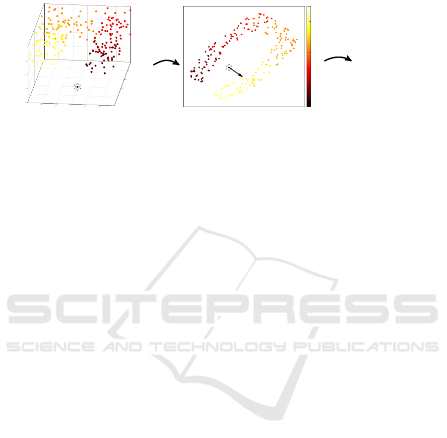
Figure 1: Illustration of the investigated topic: a ’high-dimensional’ data set (left, with an outlier marked as a star) is mapped

to two dimensions (middle), where the question ’why is the central point mapped here and not there’ is asked (indicated by

the arrow). Possible explanations are depicted (right).

and a decoder, mapping it back to the original in-

put (Goodfellow et al., 2016):

(x) = (dec

◦ enc

)(x), (3)

which are trained to optimize the reconstruction loss.

A (typically non-linear) dimensionality reduction φ(·)

based on this approach consists of the encoder map-

ping:

φ(x) = enc

(x) (4)

2.1.4 Neighbor Embeddings

The class of neighbor embedding methods constitutes

a set of non-parametric approaches that are consid-

ered as the most successful or state-of-the-art tech-

niques in many cases (Kobak and Berens, 2019; Becht

et al., 2019; Gisbrecht and Hammer, 2015). Instances

are the very popular t-Distributed Stochastic Neigh-

bor Embedding (t-SNE) and Uniform Manifold Ap-

proximation and Projection for Dimension Reduction

(UMAP) approaches (Van der Maaten and Hinton,

2008; McInnes et al., 2018). In the following, we

consider t-SNE as a representative of this class of

methods and, among its parametric extensions (Van

Der Maaten, 2009; Gisbrecht et al., 2015), the ap-

proach Parametric t-SNE (Van Der Maaten, 2009).

Parametric t-SNE, uses a neural network f

→ R

for mapping a given input x to a lower-

dimensional domain:

φ(x) = f

(x), (5)

with respect to the t-SNE cost function.

While there do exist more families of DR ap-

proaches, such as manifold embeddings (including

MVU and LLE) or discriminative/supervised DR, it

would exceed the scope of the present work to inves-

tigate all possible choices.

2.2 Contrasting Explanations

Contrasting explanations state a change to some fea-

tures of a given input such that the resulting data

point causes a different behavior of the system/model

than the original input does. Counterfactual explana-

tions (often just called counterfactuals) are the most

prominent instance of contrasting explanations (Mol-

nar, 2019). One can think of a counterfactual explana-

tion as a recommendation of actions that change the

model’s behavior/prediction. One reason why coun-

terfactual explanations are so popular is that there ex-

ists evidence that explanations used by humans are

often contrasting in nature (Byrne, 2019) – i.e. peo-

ple often ask questions like “What would have to be

different in order to observe a different outcome?”.

It was also shown that such questions are useful to

learn about an unknown functionality and exploit this

knowledge to achieve some goals (Kuhl et al., 2022a;

Kuhl et al., 2022b).

A prominent example for illustrating the concept

of a counterfactual explanation is the example of loan

application: Imagine you applied for a loan at a bank.

Now, the bank rejects your application and you would

like to know why. In particular, you would like to

know what would have to be different so that your

application would have been accepted. A possible

explanation might be that you would have been ac-

cepted if you had earned 500$ more per month and if

you had not had a second credit card.

Unfortunately, many explanation methods (in-

cluding counterfactual explanations) are lacking

uniqueness: Often there exists more than one possi-

ble & valid explanation – this is called “Rashomon

effect” (Molnar, 2019) – and in such cases, it is not

clear which or how many of the possible explanations

should be presented to the user. See Figure 2 where

we illustrate the concept of a counterfactual explana-

tion, including the existing of multiple possible and

valid counterfactuals. Most approaches ignore this

"Why Here and not There?": Diverse Contrasting Explanations of Dimensionality Reduction

Figure 2: “Rashomon effect”: Illustration of multiple pos-

sible counterfactual explanationsx

of a given samplex

orig

for a binary classiﬁer.

problem, however, there exist a few approaches that

propose to compute multiple diverse counterfactuals

to make the user aware that there exist different pos-

sible explanations (Rodriguez et al., 2021; Russell,

2019; Mothilal et al., 2020). In order to keep the ex-

planation (suggested changes) simple – i.e. we are

looking for low-complexity explanations that are easy

to understand – an obvious strategy is to look for a

small number of changes so that the resulting sample

(counterfactual) is similar/close to the original sam-

ple. This is aimed to be captured by Deﬁnition 1.

Deﬁnition 1 ((Closest) Counterfactual Explana-

tion (Wachter et al., 2017)). Assume a prediction

function (e.g. a classiﬁer) h : R

→ Y is given. Com-

puting a counterfactual x

∈ R

for a given input

x ∈ R

is phrased as an optimization problem:

argmin

x

∈R





h(x

),y



+C · θ(x

,x) (6)

where (·) denotes a loss function, y

the target pre-

diction, θ(·) a penalty for dissimilarity of x

and x,

and C > 0 denotes the regularization strength.

The counterfactuals from Deﬁnition 1 are also

called closest counterfactuals because the optimiza-

tion problem Eq. (6) tries to ﬁnd an explanation x

that is as close as possible to the original sample x.

However, other aspects like plausibility and action-

ability are ignored in Deﬁnition 1, but are covered in

other work (Looveren and Klaise, 2019; Artelt and

Hammer, 2020; Artelt and Hammer, 2021). In this

work, we refer to counterfactuals in the spirit of Def-

inition 1. Note that counterfactual explanations also

exist in the causality domain (Pearl, 2010). Here

the knowledge of a structural causal model (SCM),

describing the interaction of features, is assumed.

This work is not based in the causality domain and

we only consider counterfactual explanations as pro-

posed by (Wachter et al., 2017).

3 COUNTERFACTUAL

EXPLANATIONS OF

DIMENSIONALITY

REDUCTION

In this section, we propose counterfactual explana-

tions of dimensionality reduction – i.e. explaining

why a speciﬁc point was mapped to some location in-

stead of a requested different location. As it is the na-

ture of counterfactual explanations, the explanations

state how we have to (minimally) change the original

sample such that it gets mapped to some requested lo-

cation – see Figure 1 for an illustrative example.

We argue that this type of explanation is in partic-

ular very well suited for explaining data visualization

which is a common application of dimensionality re-

duction in data mining (Gisbrecht and Hammer, 2015;

Lee and Verleysen, 2007; Kaski and Peltonen, 2011)

– e.g. data is mapped to a two-dimensional space

which is then depicted in a scatter plot. For instance,

we could utilize such explanations to explain outliers

in the data visualization: I.e. explaining why a point

got mapped far away from the other points instead

of close to the other ones – a counterfactual expla-

nation states how to change the outlier such that it is

no longer an outlier in the visualization, which would

allow us to learn something about the particular rea-

sons why this point was ﬂagged as an outlier in the

visualization. See Figure 3 for an illustrative exam-

ple where we explain anomalous pressure measure-

ments in a water distribution network: We consider

the hydraulically isolated “Area A” in the L-Town net-

work (Vrachimis et al., 2020) where 29 pressure sen-

sors are installed – we simulate a sensor failure (con-

stant added the original pressure value) in node n105.

We pick an outlier x (see left plot in Figure 3) and

compute a counterfactual explanation for each normal

data point as a target mapping – i.e. asking which sen-

sor measurements must be changed so that the over-

all measurement vector x

is mapped to the speciﬁed

location in the data visualization. When aggregating

all explanations by summing up and normalizing the

suggested changes for each sensor (see right plot in

Figure 3), we are able to identify the faulty sensors

and thereby “explain” the outlier.

Note that existing explanation methods for ex-

plaining dimensionality reduction methods, which

usually focus on feature importances (see Section 1),

can not provide such an explanation – i.e. answer-

ICPRAM 2023 - 12th International Conference on Pattern Recognition Applications and Methods

Figure 3: Explaining anomalous pressure measurements – Left: Two dimensional data visualization of 29-dimensional pres-

sure measurements; Right: Normalized amount of suggested changes per sensor – the faulty sensor is suggested to change the

most and is therefore correctly identiﬁed.

ing contrasting questions like “Why was the point

mapped here and not there”. This is because they only

highlight important features but do not suggest any

changes or magnitude of changes that would yield a

different (requested) mapping. However, as already

mentioned in Section 2.2, the Rashomon effect states

that there might exist many possible explanations why

a particular point was mapped far away from the oth-

ers – we therefore aim for a set of diverse counterfac-

tual explanations in order to learn the most about the

observed mapping and provide different possibilities

for actionable recourse.

First, we formalize the general concept of (di-

verse) counterfactual explanations of dimensionality

reduction in Section 3.1. Next, we consider some

popular parametric dimensionality reduction meth-

ods, and propose methods for efﬁciently computing

single counterfactuals (see Section 3.2) and diverse

counterfactuals (see Section 3.3).

3.1 General Modeling

We assume the DR method is given as a mapping

φ : R

→ R

(7)

with d > d

A counterfactual explanation of a sample x ∈ R

is a sample x

in the original domain (i.e. R

) that

differs in a few features only from the given origi-

nal sample x, but is mapped to a requested location

y

∈ R

which is different from the mapping of the

original sample x. We formalize this in Deﬁnition 2.

Deﬁnition 2 (Counterfactual Explanation of Di-

mensionality Reduction). For a given DR method

φ(·) Eq. (7), a counterfactual explanation x

∈

,y

∈ R

of a speciﬁc sample x ∈ R

is given as

a solution to the following multi-criteria optimization

problem:

min

x

∈R



kx −x

,kφ(x

) −y



, (8)

where p deﬁnes the norm that is used. As

discussed in Section 2.2, there usually exists more

than one possible explanation (“Rashomon effect”) –

clearly this is the case for dimensionality reduction as

well because dimensionality reduction is a many-to-

one mapping (i.e. multiple points are mapped to the

same location). In this context, a set of diverse (i.e.

highly different) explanations would provide more in-

formation than a single explanation only. We there-

fore extend Deﬁnition 2 to a set of diverse counter-

factuals explanations instead of a single one:

Deﬁnition 3 (Diverse Counterfactual Explanations of

Dimensionality Reduction). For a given DR method

φ(·) Eq. (7), a set of diverse counterfactual explana-

tions {x

∈ R

},y

∈ R

of a speciﬁc samplex ∈ R

is given as a solution to the following multi-criteria

optimization problem:

min

{x

∈R

}



kx −x

,kφ(x

) −y

,ψ(x

,x

)



(9)

where ψ : R

× R

→ R

denotes a function measur-

ing the pair-wise diversity of two given counterfactu-

als – i.e. returning a small value if the two counterfac-

tuals are very different and a larger value otherwise.

The term “diversity” itself is somewhat fuzzy and

different use-cases might require different deﬁnitions

of diverse counterfactuals. In this work we utilize a

very general deﬁnition of diversity, namely the num-

ber of overlapping features – i.e. diverse counterfac-

"Why Here and not There?": Diverse Contrasting Explanations of Dimensionality Reduction

tuals should not change the same features:

ψ(x

,x

) =

∑

i=1



(



)

6= 0 ∧ (



)

6= 0



(10)

where



= x

−x and 1(·) denotes the indicator

function that returns 1 if the boolean expression is true

and 0 otherwise.

3.2 Method Speciﬁc Computation of a

Single Counterfactual

Hereinafter, we propose practical relaxations for com-

puting a single counterfactual explanation of dif-

ferent parametric dimensionality reduction methods

(see Deﬁnition 2). While Deﬁnition 2 does not make

any assumptions on the dimensionality reduction φ(·),

we now assume a parametric dimensionality reduc-

tion in order to get tractable optimization problems.

Note that in all cases, we approximate the 0-norm

with the 1-norm for measuring closeness between the

original sample x and the counterfactual x

. Further-

more, we use p = 2, the 2-norm for measuring the

distance between the mapping ofx

and the requested

mapping y

3.2.1 Linear Methods

In the case of linear mappings as deﬁned in Sec-

tion 2.1.1, we phrase the computation of a single

counterfactual explanations as the following convex

quadratic program:

argmin

x

∈R

kx −x

+C · ξ

s.t. kAx



b −y

≤ ξ

ξ ≥ 0

(11)

where C > 0 acts as a regularization strength balanc-

ing between the two objectives in Eq. (8) – the regu-

larization is necessary because it is numerically difﬁ-

cult (or even impossible) to ﬁnd a counterfactual x

that yields the exact mapping φ(x

) =y

, we there-

fore have to specify how much difference we are will-

ing to tolerate. Note that convex quadratic programs

can be solved efﬁciently (Boyd and Vandenberghe,

2004).

3.2.2 Self Organizing Map

Similar to linear methods, we phrase the computa-

tion of a single counterfactual explanations for SOMs

(Section 2.1.2) as the following convex quadratic pro-

gram, which again can be solved efﬁciently using

standard solvers from convex optimization (Boyd and

Vandenberghe, 2004):

argmin

x

∈R

kx −x

s.t. kx

−p

y

+ ε ≤ kx

−p

z

∀z ∈ I

(12)

where ε > 0 makes sure that the set of feasible solu-

tions is closed.

3.2.3 Autoencoder

For autoencoders (AEs) as discussed in Section 2.1.3,

we utilize the penalty method to merge the two objec-

tives from Eq. (8) into a single objective:

argmin

x

∈R

kx −x

+C · kenc

(x

) −y

(13)

where the hyperparameter C > 0 acts as a regulariza-

tion strength.

Assuming continuous differentiability of the en-

coder enc

(·), we can solve Eq. (13) using a gradient

based method. However, due to the non-linearity of

enc

(·), we might ﬁnd a local optimum only.

3.2.4 Parametric t-SNE

Although the neural network f

(·) of parametric t-

SNE (Section 2.1.4) is trained in a completely differ-

ent way compared to an autoencoder based dimen-

sionality reduction, the ﬁnal modeling is the same

and consequently, everything from the case of autoen-

coder based DR applies here as well:

argmin

x

∈R

kx −x

+C · k f

(x

) −y

(14)

3.3 Computation of Diverse

Counterfactuals

In this section, we propose an algorithm for comput-

ing diverse counterfactual explanations (see Deﬁni-

tion 3) of the four DR methods considered in the pre-

vious section.

Regarding the formalization of diversity Eq. (10),

instead of using Eq. (10) directly, we propose a more

stricter version in order to get a continuous func-

tion which then yields tractable optimization prob-

lems, similar to the ones we proposed in the pre-

vious section: In order to compute a set of diverse

counterfactuals instead of a single counterfactual, we

utilize our proposed methods for computing a sin-

gle counterfactual explanations from Section 3.2 and

extend these with a mechanism to forbid or punish

changes in black-listed features. We then ﬁrst com-

pute a single counterfactual explanations using the

ICPRAM 2023 - 12th International Conference on Pattern Recognition Applications and Methods

Algorithm 1: Computation of Diverse Counterfactuals.

Input: Original input x, Target location y

, k ≥ 1:

number of diverse counterfactuals, Dimensionality re-

duction φ(·)

Output: Set of diverse counterfactuals R = {x

}

1: F = {}  Initialize set of black-listed features

2: R = {}  Initialize set of diverse counterfactuals

3: for i = 1,...,k do  Compute k diverse

counterfactuals

4: x

= CF

(x,y

,F )  Compute next

counterfactual

5: R = R ∪ {x

}

6: F = F ∪ { j | (x

−x)

6= 0}  Update set of

black-listed features

7: end for

methodology proposed in Section 3.2 and then itera-

tively compute another counterfactual explanation but

black-listing all features that have been changed in the

previous counterfactuals – this procedure is illustrated

as pseudo-code in Algorithm 1.

Black-Listing Features. We assume we are given

an ordered set F of black-listed features. In case of

convex programs (e.g. linear methods and SOM), we

consider black-listed features F by means of an addi-

tional afﬁne equality constraint:

Mx

= m (15)

where M ∈ R

|F |×d

,m ∈ R

|F |

with

(M)

i, j

(

1 if (F )

= j

0 otherwise

(16)

and m

= (x)

(F )

Whereas in all other cases (e.g. autoencoder

and parametric t-SNE), where we minimize a (non-

convex) cost function, we replace the counterfactual

x

in the optimization problem with an afﬁne map-

ping undoing any potential changes in black-listed

features – i.e. black-listed features can be changed

but have no effect on the ﬁnal counterfactual because

they are reset to their original value:

kφ(Mx

+m)−y

(17)

where M ∈ R

d×d

,m ∈ R

with

(M)

i, j

(

1 if i = j and i 6∈ F

0 otherwise

(m)

(

(x)

if i ∈ F

0 otherwise

(18)

Note that in both cases, the complexity and type of

optimization problem does not change – e.g. convex

programs remain convex programs.

For convenience, we use CF

(x,y

,F ) to denote

the computation of a counterfactual (x

,y

) of a DR

method φ(·) at a given sample x subject to a set F of

black-listed features.

4 EXPERIMENTS

We empirically evaluate our proposed explanation

methodology of DR methods on the speciﬁc use-case

of data visualization – i.e. dimensionality reduction

to two dimensions. All experiments are implemented

in Python and are publicly available on GitHub

4.1 Data

We run all our experiments on a set of different ML

benchmark data sets – all data sets are standardized:

Diabetes. The “Diabetes Data Set” (N/A, 1994) is

a labeled data set containing recordings from diabetes

patients. The data set contains 442 samples and 10

real valued scaled features in [−.2,.2] such as body

mass index, age in years and average blood pressure.

The labels are integers in [25, 346] denoting a quan-

titative measure of disease progression one year after

baseline.

Breast Cancer. The “Breast Cancer Wisconsin (Di-

agnostic) Data Set” (William H. Wolberg, 1995) is

used for classifying breast cancer samples into benign

and malignant (i.e. binary classiﬁcation). The data set

contains 569 samples and 30 numerical features such

as area, smoothness and compactness.

Toy. An an artiﬁcial, self created, toy data set con-

taining 500 ten dimensional samples. Each fea-

ture is distributed according to a normal distribution

whereby we choose a different random mean for each

feature - by this we can guarantee that, in contrast to

the other data sets, the features are independent of

each other. The binary labelling of the samples is

done by splitting the data into two clusters using k-

means.

4.2 Model Agnostic Algorithm for

Comparison

We compare Algorithm 1 to a general model agnos-

tic algorithm (ModelAgnos) for computing diverse

https://github.com/HammerLabML/ContrastingExpl

anationDimRed

"Why Here and not There?": Diverse Contrasting Explanations of Dimensionality Reduction

counterfactual explanations where we select samples

from the training data set D that minimize a weighted

combination of Eq. (9) – i.e. we make use of the

penalty method to solve the multi-objective optimiza-

tion problem Eq. (9) without making any further as-

sumption on the dimensionality reduction φ(·):

min

{x

∈D}

· kx −x

· kφ(x

) −y

· ψ(x

,x

)

(19)

where C

> 0 denote regularization coefﬁ-

cients that allow us to balance between the differ-

ent objectives, and ψ(·) is implemented as stated

in Eq. (10). By limiting the set of feasible solutions to

the training data set, we can guarantee plausibility of

the resulting counterfactual explanations – note that

plausibility of the counterfactuals generated by Algo-

rithm 1 can not be guaranteed.

4.3 Setup

For each data set and each of the four parametric

DR methods (PCA, Autoencoder, SOM, parametric

t-SNE) from Section 3.2, we ﬁt the DR method to the

entire data set and compute for each sample in the data

set a set of three diverse counterfactual explanations

– we evaluate and compare the counterfactuals

com-

puted by our proposed Algorithm 1 with those from

the model agnostic algorithm (see Section 4.2). For

the requested target locationy

– recall that in a coun-

terfactual explanation we ask for a change that would

lead to a different speciﬁed mappingy

instead of the

original mapping y – we consider two scenarios:

• Perturbations: Choose the mapping of the orig-

inal sample x after perturbing three random fea-

tures – the same type of perturbation is applied to

these three features.

• Without any perturbations: Choose the mapping

of a different sample (with a different label) from

the training data set as y

Regarding the perturbations, we consider the follow-

ing ones:

• Shift: A constant is added to the feature value.

• Gaussian: Gaussian noise is added to feature

value.

Note that we evaluate each perturbation separately.

Furthermore, note that these perturbations could be

interpreted as sensor failures and are therefore highly

relevant to practice.

All hyperparameters (regularization strength) C

∀i are

set to 1.

4.4 Evaluation

For all experimental scenarios, we monitor and eval-

uate some quantitative measurements:

• CfSparse: Sparsity of the counterfactual explana-

tions – i.e. how many (percentage) of the avail-

able features are used in the explanation, smaller

values are better.

• CfDist: Euclidean distance between the mapping

of the counterfactual φ(x

) and the requested

mapping y

– i.e. this can be interpreted as a

measurement of the error of counterfactual expla-

nations, smaller values are better.

• CfDiv: Diversity of the counterfactual explana-

tions – i.e. the number of overlapping features

between the diverse explanations (see Eq. (10) in

Section 3.1), smaller values are better.

For the scenarios where we apply a perturbation to

the original sample, we also record the recall of the

identiﬁed perturbed features in the counterfactual ex-

planations – i.e. checking if the used features in the

explanation coincide with the perturbed features. By

this, we try to measure the usefulness of our explana-

tions for identifying relevant features – however, since

dimensionality reduction is a many-to-one mapping,

we consider recall only because we do not expect to

observe a high precision due to the Rashomon effect.

Note that each experiment is repeated 100 times

in order to get statistically reliable estimates of the

quantitative measurements.

4.5 Results

The results of the scenario without any perturbations

– i.e. randomly selecting the target sample from the

training set – are shown in Table 1 and the results

of the scenarios with perturbations are shown in Ta-

bles 6,2 – note that, due to space constraints, the latter

one is put in the appendix.

We observe that Algorithm 1, on average, achieves

much sparser and more diverse explanations than the

mode agnostic algorithm (Section 4.2) does. Only in

case of SOM, the sparsity is often a bit worse than

those from the baseline – this might be due to numeri-

cal instabilities of the mathematical program Eq. (12).

In particular, while Algorithm 1 almost always yields

completely diverse explanations, the model agnos-

tic algorithm fails completely – this highlights the

strength of our proposed Algorithm 1 for computing

diverse explanations. Furthermore, both methods are

able to yield counterfactual explanations that are very

close to the requested target location. In most cases

Algorithm 1 yields counterfactuals that are closer to

ICPRAM 2023 - 12th International Conference on Pattern Recognition Applications and Methods

Table 1: Quantitative results: No perturbation – all numbers are rounded to two decimal places, best scores are highlighted in

bold-face.

DataSet

CfSparse ↓ CfDiv ↓ CfDist ↓

Algo 1 ModelAgnos Algo 1 ModelAgnos Algo 1 ModelAgnos

Linear

Diabetes 0.21 ± 0.0 0.55 ± 0.0 0.0 ± 0.0 7.07 ± 0.86 0.2 ± 0.2 1.33 ± 0.39

Breast cancer 0.15 ± 0.01 0.66 ± 0.0 0.0 ± 0.0 29.6 ± 0.89 0.36 ± 1.47 2.64 ± 1.5

Toy 0.21 ± 0.0 0.67 ± 0.0 0.0 ± 0.0 9.99 ± 0.01 0.03 ± 0.04 0.85 ± 0.12

SOM

Diabetes 0.88 ± 0.02 0.61 ±0.01 0.0 ± 0.0 9.63 ± 21.16 0.01 ± 0.15 3.2 ± 2.73

Breast cancer 0.91 ± 0.02 0.66 ± 0.0 0.0 ± 0.04 29.71 ±0.62 0.4 ± 5.22 4.07 ± 3.91

Toy 0.84 ± 0.03 0.68 ± 0.0 0.0 ± 0.0 10.6 ± 11.73 0.01 ± 0.17 3.77 ± 3.18

Diabetes 0.14 ± 0.03 0.51 ± 0.0 0.0 ± 0.01 6.15 ± 0.7 0.28 ± 0.08 0.23 ± 0.04

Breast cancer 0.03 ± 0.01 0.65 ± 0.0 0.0 ± 0.05 28.95 ±0.92 0.36 ± 0.16 0.31 ± 0.12

Toy 0.14 ± 0.03 0.67 ± 0.0 0.0 ± 0.02 9.98 ± 0.02 0.3 ± 0.09 0.18 ± 0.02

t-SNE

Diabetes 0.33 ± 0.0 0.58 ± 0.0 0.0 ± 0.0 8.12 ± 1.11 5.35 ± 7.43 3.0 ± 1.83

Breast cancer 0.32 ± 0.01 0.67 ± 0.0 0.23 ± 4.74 29.86 ± 0.17 8.52 ± 11.59 4.32 ±2.16

Toy 0.33 ± 0.0 0.67 ± 0.0 0.0 ± 0.0 10.0 ± 0.0 1.92 ± 0.81 1.06 ± 0.21

the target location, only in case of parametric t-SNE

the model agnostic algorithm yields “better” coun-

terfactuals – however, in both cases the variance is

quite large which indicates instabilities of the learned

dimensionality reduction. Note that, since the three

evaluation metrics 4.4 are contradictory, it can be mis-

leading to evaluate the performance under each met-

ric separately without looking at the other metrics

at the same time – e.g. a method might yield very

sparse counterfactuals but their distance to the re-

questing mappings is very large. In order to compen-

sate the contradictory nature of the evaluation metrics,

we suggest to also consider a ranking over the three

metrics when assessing the performance of the two

proposed algorithms for computing counterfactuals –

we give such a ranking in Tables 3,4,5. According to

these rankings, Algorithm 1 outperforms the model

agnostic algorithm in many cases or is at at least as

good as the model agnostic method but never worse.

While the recall of the baseline is very good across all

DR methods and data sets, the recall of Algorithm 1

is often very good as well, however, there exist some

cases (in particular the breast cancer data set) where

the recall drops signiﬁcantly compared to the model

agnostic algorithm.

5 CONCLUSION

In this work, we proposed the abstract concept of con-

trasting explanations for locally explaining dimen-

sionality reduction methods – we considered two-

dimensional data visualization as a popular example

application. In order to deal with the Rashomon ef-

fect – i.e. the fact that there exist more than one

possible and valid explanation – we considered a set

of diverse explanations instead of a single explana-

tion. Furthermore, we also proposed an implementa-

tion of this concept using counterfactual explanations

and proposed modelings and algorithms for efﬁciently

computing diverse counterfactual explanations of dif-

ferent parametric dimensionality reduction methods.

We empirically evaluated different aspects of our pro-

posed algorithms on different standard benchmark

data sets – we observe that our proposed methods con-

sistently yield good results.

Based on this initial work, there are a couple

of potential extensions and directions for future re-

search:

Depending on the domain and application, it

might be necessary to guarantee plausibility of the

counterfactuals – i.e. making sure that the counterfac-

tualx

is reasonable and plausible in the data domain.

Implausibility or a lack of realism of the counterfac-

tual x

might hinder successful recourse in practice.

In this work, we ignored the aspect of plausibility and

it might happen that the computed counterfactuals x

are not always realistic samples from the data domain

– only in case of our model agnostic algorithm (see

Section 4.2) we can guarantee plausibility because

we only consider samples from the training data set

D as potential counterfactuals x

. In future work, a

ﬁrst approach could be to add plausibility constraints

to our proposed modelings (see Section 3.1) like it

was done for counterfactual explanations of classi-

ﬁers (Artelt and Hammer, 2020; Artelt and Hammer,

2021; Looveren and Klaise, 2019).

Another crucial aspects of transparency & ex-

plainability is the human. In particular, quantitative

evaluation of algorithmic properties do not necessary

coincide with a human evaluation (Kuhl et al., 2022a).

Therefore we suggest to conduct a user-study to eval-

uate how “useful” our proposed explanation actually

are – in particular it would be of interest to compare

normal vs. plausible explanations, and to compare di-

verse explanations vs. a single explanations.

"Why Here and not There?": Diverse Contrasting Explanations of Dimensionality Reduction

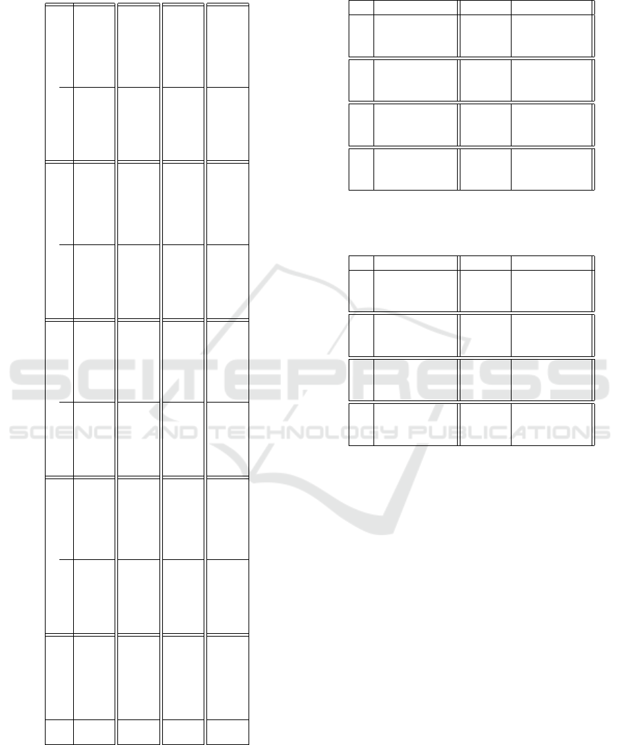
Table 2: Quantitative results: Shift perturbation – all num-

bers are rounded to two decimal places, best scores are high-

lighted in bold-face.

DataSet

CfSparse ↓ CfDiv ↓ CfDist ↓ Recall ↑

Algo 1 ModelAgnos Algo 1 ModelAgnos Algo 1 ModelAgnos Algo 1 ModelAgnos

Linear

Diabetes 0.23 ± 0.0 0.56 ± 0.0 0.0 ± 0.0 7.44 ± 0.82 0.28 ± 0.37 2.86 ± 1.42 0.72 ± 0.07 0.95 ± 0.02

Breast cancer 0.11 ± 0.01 0.66 ± 0.0 0.0 ± 0.0 29.48 ± 1.02 0.02 ± 0.02 1.56 ± 0.26 0.42 ± 0.09 1.0 ± 0.0

Toy 0.21 ± 0.0 0.67 ± 0.0 0.0 ± 0.0 10.0 ± 0.0 0.01 ± 0.03 2.34 ± 2.21 0.8 ± 0.04 1.0 ±0.0

SOM

Diabetes 0.8 ± 0.04 0.6 ± 0.01 0.0 ± 0.01 9.31 ± 20.54 0.01 ± 0.09 3.74 ± 3.72 0.94 ± 0.02 0.96 ± 0.01

Breast cancer 0.67 ± 0.07 0.66 ± 0.0 0.01 ± 0.18 29.68 ± 0.84 0.31 ±4.04 4.6 ± 13.18 0.95 ± 0.02 1.0 ± 0.0

Toy 0.77 ± 0.04 0.67 ± 0.0 0.0 ± 0.01 10.47 ±9.14 0.02 ± 0.25 3.67 ± 3.3 0.92 ± 0.03 1.0 ± 0.0

Diabetes 0.14 ± 0.03 0.51 ± 0.0 0.0 ± 0.03 6.21 ± 0.71 0.78 ± 0.6 0.74 ± 0.63 0.43 ± 0.24 0.9 ± 0.03

Breast cancer 0.04 ± 0.01 0.65 ± 0.0 0.0 ± 0.04 28.98 ± 0.94 0.47 ± 0.24 0.51 ± 0.24 0.13 ±0.1 1.0 ± 0.0

Toy 0.16 ± 0.03 0.67 ± 0.0 0.0 ± 0.01 9.97 ± 0.03 0.62 ± 0.26 0.57 ±0.39 0.48 ± 0.25 1.0 ± 0.0

t-SNE

Diabetes 0.33 ± 0.0 0.58 ± 0.0 0.01 ± 0.09 8.06 ± 0.91 6.13 ± 8.14 4.4 ± 5.63 1.0 ±0.0 0.96 ± 0.01

Breast cancer 0.32 ± 0.0 0.66 ± 0.0 0.08 ± 1.42 29.65 ± 0.95 3.14 ± 2.2 2.0 ± 0.55 0.97 ± 0.02 1.0 ± 0.0

Toy 0.33 ± 0.0 0.67 ± 0.0 0.0 ± 0.0 10.0 ± 0.0 2.81 ± 1.46 1.87 ± 0.97 1.0 ± 0.0 1.0 ± 0.0

Table 3: Ranking of results from Table 1 – counting the

number of metrics where the method yields the best score,

best scores are highlighted in bold-face.

DataSet Algo 1 ModelAgnos

Linear

Diabetes 3/3 0/3

Breast cancer 3/3 0/3

Toy 3/3 0/3

SOM

Diabetes 2/3 1/3

Breast cancer 2/3 1/3

Toy 2/3 1/3

Diabetes 2/3 1/3

Breast cancer 2/3 1/3

Toy 2/3 1/3

t-SNE

Diabetes 2/3 1/3

Breast cancer 2/3 1/3

Toy 2/3 1/3

Table 4: Ranking of results from Table 2 – counting the

number of metrics where the method yields the best score,

best scores are highlighted in bold-face.

DataSet Algo 1 ModelAgnos

Linear

Diabetes 3/4 1/4

Breast cancer 3/4 1/4

Toy 3/4 1/4

SOM

Diabetes 2/4 2/4

Breast cancer 2/4 2/4

Toy 2/4 2/4

Diabetes 2/4 2/4

Breast cancer 3/4 1/4

Toy 2/4 2/4

t-SNE

Diabetes 3/4 1/4

Breast cancer 2/4 2/4

Toy 3/4 1/4

ACKNOWLEDGEMENTS

We gratefully acknowledge funding from the VW-

Foundation for the project IMPACT funded in the

frame of the funding line AI and its Implications for

Future Society.

REFERENCES

Aamodt, A. and Plaza., E. (1994). Case-based reasoning:

Foundational issues, methodological variations, and

systemapproaches. AI communications.

Artelt, A. and Hammer, B. (2020). Convex density con-

straints for computing plausible counterfactual expla-

nations. 29th International Conference on Artiﬁcial

Neural Networks (ICANN).

Artelt, A. and Hammer, B. (2021). Convex optimization for

actionable \& plausible counterfactual explanations.

CoRR, abs/2105.07630.

Bach, S., Binder, A., Montavon, G., Klauschen, F., M

uller,

K.-R., and Samek, W. (2015). On pixel-wise explana-

ICPRAM 2023 - 12th International Conference on Pattern Recognition Applications and Methods

tions for non-linear classiﬁer decisions by layer-wise

relevance propagation. PloS one, 10(7):e0130140.

Bardos, A., Mollas, I., Bassiliades, N., and Tsoumakas, G.

(2022). Local explanation of dimensionality reduc-

tion. arXiv preprint arXiv:2204.14012.

Becht, E., McInnes, L., Healy, J., Dutertre, C.-A., Kwok,

I. W., Ng, L. G., Ginhoux, F., and Newell, E. W.

(2019). Dimensionality reduction for visualizing

single-cell data using umap. Nature biotechnology,

37(1):38–44.

Bibal, A., Vu, V. M., Nanfack, G., and Fr

enay, B.

(2020). Explaining t-sne embeddings locally by adapt-

ing lime. In ESANN, pages 393–398.

Boyd, S. and Vandenberghe, L. (2004). Convex Optimiza-

tion. Cambridge University Press, New York, NY,

USA.

Bunte, K., Biehl, M., and Hammer, B. (2012). A gen-

eral framework for dimensionality-reducing data visu-

alization mapping. Neural Computation, 24(3):771–

804.

Byrne, R. M. J. (2019). Counterfactuals in explainable ar-

tiﬁcial intelligence (xai): Evidence from human rea-

soning. In IJCAI-19.

Doshi-Velez, F. and Kim, B. (2017). Towards a rigorous

science of interpretable machine learning.

Fisher, A., Rudin, C., and Dominici, F. (2018). All Models

are Wrong but many are Useful: Variable Importance

for Black-Box, Proprietary, or Misspeciﬁed Prediction

Models, using Model Class Reliance. arXiv e-prints,

page arXiv:1801.01489.

Gisbrecht, A. and Hammer, B. (2015). Data visualization

by nonlinear dimensionality reduction. Wiley Interdis-

ciplinary Reviews: Data Mining and Knowledge Dis-

covery, 5(2):51–73.

Gisbrecht, A., Schulz, A., and Hammer, B. (2015). Para-

metric nonlinear dimensionality reduction using ker-

nel t-sne. Neurocomputing, 147:71–82.

Goodfellow, I., Bengio, Y., and Courville, A. (2016). Deep

learning. MIT press.

Kaski, S. and Peltonen, J. (2011). Dimensionality reduc-

tion for data visualization [applications corner]. IEEE

signal processing magazine, 28(2):100–104.

Kim, B., Koyejo, O., and Khanna, R. (2016). Examples

are not enough, learn to criticize! criticism for inter-

pretability. In Advances in Neural Information Pro-

cessing Systems 29.

Kobak, D. and Berens, P. (2019). The art of using t-sne for

single-cell transcriptomics. Nature communications,

10(1):1–14.

Kohonen, T. (1990). The self-organizing map. Proceedings

of the IEEE, 78(9):1464–1480.

Kuhl, U., Artelt, A., and Hammer, B. (2022a). Keep

your friends close and your counterfactuals closer:

Improved learning from closest rather than plausi-

ble counterfactual explanations in an abstract setting.

arXiv preprint arXiv:2205.05515.

Kuhl, U., Artelt, A., and Hammer, B. (2022b). Let’s go to

the alien zoo: Introducing an experimental framework

to study usability of counterfactual explanations for

machine learning. arXiv preprint arXiv:2205.03398.

Lapuschkin, S., W

aldchen, S., Binder, A., Montavon, G.,

Samek, W., and M

uller, K.-R. (2019). Unmasking

clever hans predictors and assessing what machines

really learn. Nature communications, 10(1):1–8.

Lee, J. A. and Verleysen, M. (2007). Nonlinear dimension-

ality reduction, volume 1. Springer.

Looveren, A. V. and Klaise, J. (2019). Interpretable coun-

terfactual explanations guided by prototypes. CoRR,

abs/1907.02584.

McInnes, L., Healy, J., and Melville, J. (2018). Umap: Uni-

form manifold approximation and projection for di-

mension reduction. arXiv preprint arXiv:1802.03426.

Molnar, C. (2019). Interpretable Machine Learning.

Mothilal, R. K., Sharma, A., and Tan, C. (2020). Explain-

ing machine learning classiﬁers through diverse coun-

terfactual explanations. In Proceedings of the 2020

Conference on Fairness, Accountability, and Trans-

parency, pages 607–617.

N/A (1994). Diabetes data set. https://www4.stat.ncsu.edu

∼

boos/var.select/diabetes.html.

Offert, F. (2017). ”i know it when i see it”. visualization and

intuitive interpretability.

parliament, E. and council (2016). General data protection

regulation: Regulation (eu) 2016/679 of the european

parliament.

Pearl, J. (2010). Causal inference. Causality: objectives

and assessment, pages 39–58.

Ribera, M. and Lapedriza, A. (2019). Can we do better

explanations? a proposal of user-centered explainable

ai. In IUI Workshops, volume 2327, page 38.

Rodriguez, P., Caccia, M., Lacoste, A., Zamparo, L.,

Laradji, I., Charlin, L., and Vazquez, D. (2021).

Beyond trivial counterfactual explanations with di-

verse valuable explanations. In Proceedings of the

IEEE/CVF International Conference on Computer Vi-

sion, pages 1056–1065.

Russell, C. (2019). Efﬁcient search for diverse coherent ex-

planations. In Proceedings of the Conference on Fair-

ness, Accountability, and Transparency, pages 20–28.

Samek, W., Wiegand, T., and M

uller, K. (2017). Explain-

able artiﬁcial intelligence: Understanding, visualiz-

ing and interpreting deep learning models. CoRR,

abs/1708.08296.

Schulz, A., Gisbrecht, A., and Hammer, B. (2014). Rel-

evance learning for dimensionality reduction. In

ESANN, pages 165–170. Citeseer.

Schulz, A. and Hammer, B. (2015). Metric learning in di-

mensionality reduction. In ICPRAM (1), pages 232–

239.

Schulz, A., Hinder, F., and Hammer, B. (2021). Deepview:

visualizing classiﬁcation boundaries of deep neural

networks as scatter plots using discriminative dimen-

sionality reduction. In Proceedings of IJCAI, pages

2305–2311.

Tjoa, E. and Guan, C. (2019). A survey on explainable

artiﬁcial intelligence (XAI): towards medical XAI.

CoRR, abs/1907.07374.

Van Der Maaten, L. (2009). Learning a parametric embed-

ding by preserving local structure. In Artiﬁcial intelli-

gence and statistics, pages 384–391. PMLR.

"Why Here and not There?": Diverse Contrasting Explanations of Dimensionality Reduction

Van der Maaten, L. and Hinton, G. (2008). Visualizing data

using t-sne. Journal of machine learning research,

9(11).

Van Der Maaten, L., Postma, E., Van den Herik, J., et al.

(2009). Dimensionality reduction: a comparative. J

Mach Learn Res, 10(66-71):13.

Verma, S., Dickerson, J., and Hines, K. (2020). Counterfac-

tual explanations for machine learning: A review.

Vrachimis, S. G., Eliades, D. G., Taormina, R., Ostfeld, A.,

Kapelan, Z., Liu, S., Kyriakou, M., Pavlou, P., Qiu,

M., and Polycarpou, M. M. (2020). Battledim: Battle

of the leakage detection and isolation methods.

Wachter, S., Mittelstadt, B., and Russell, C. (2017). Coun-

terfactual explanations without opening the black box:

Automated decisions and the gdpr. Harv. JL & Tech.,

31:841.

William H. Wolberg, W. Nick Street, O. L. M. (1995).

Breast cancer wisconsin (diagnostic) data set. https:

//archive.ics.uci.edu/ml/datasets/Breast+Cancer+Wi

sconsin+(Diagnostic).

APPENDIX

Results of the Empirical Evaluation

Table 5: Ranking of results from Table 6 – counting the

number of metrics where the method yields the best score,

best scores are highlighted in bold-face.

DataSet Algo 1 ModelAgnos

Linear

Diabetes 3/4 1/4

Breast cancer 3/4 1/4

Toy 3/4 1/4

SOM

Diabetes 2/4 2/4

Breast cancer 2/4 2/4

Toy 2/4 2/4

Diabetes 2/4 2/4

Breast cancer 2/4 2/4

Toy 2/4 2/4

t-SNE

Diabetes 3/4 1/4

Breast cancer 2/4 2/4

Toy 3/4 1/4

Table 6: Quantitative results: Gaussian perturbation – all

numbers are rounded to two decimal places, best scores are

highlighted in bold-face.

DataSet

CfSparse ↓ CfDiv ↓ CfDist ↓ Recall ↑

Algo 1 ModelAgnos Algo 1 ModelAgnos Algo 1 ModelAgnos Algo 1 ModelAgnos

Linear

Diabetes 0.22 ± 0.0 0.55 ± 0.0 0.0 ± 0.0 7.14 ± 0.93 0.57 ± 2.23 4.24 ± 49.13 0.7 ± 0.07 0.93 ± 0.02

Breast cancer 0.09 ± 0.0 0.66 ± 0.0 0.0 ± 0.0 29.43 ± 1.03 0.05 ± 0.21 1.35 ± 1.7 0.36 ± 0.09 1.0 ± 0.0

Toy 0.22 ± 0.0 0.67 ± 0.0 0.0 ± 0.0 10.0 ± 0.0 0.16 ± 0.62 2.99 ± 12.53 0.57 ±0.12 1.0 ±0.0

SOM

Diabetes 0.79 ± 0.05 0.6 ± 0.01 0.0 ± 0.01 9.15 ± 19.24 0.02 ± 0.2 3.84 ± 3.93 0.92 ± 0.03 0.94 ± 0.02

Breast cancer 0.6 ± 0.07 0.66 ± 0.0 0.01 ± 0.2 29.66 ±0.9 0.28 ± 3.74 3.87 ± 14.26 0.95 ± 0.02 1.0 ± 0.0

Toy 0.74 ± 0.06 0.68 ± 0.0 0.0 ± 0.01 10.55 ± 10.66 0.01 ± 0.09 3.68 ± 3.82 0.9 ± 0.04 1.0 ± 0.0

Diabetes 0.14 ± 0.03 0.51 ± 0.0 0.0 ± 0.01 6.23 ±0.69 1.09 ± 5.81 1.07 ± 3.78 0.43 ± 0.24 0.91 ±0.03

Breast cancer 0.04 ± 0.01 0.65 ± 0.0 0.0 ± 0.03 28.98 ± 0.94 0.48± 0.51 0.38 ± 0.22 0.11 ± 0.09 1.0 ± 0.0

Toy 0.14 ± 0.03 0.67 ± 0.0 0.0 ± 0.01 9.98 ±0.02 0.99 ± 3.21 0.5 ± 0.99 0.42 ± 0.24 1.0 ± 0.0

t-SNE

Diabetes 0.33 ± 0.0 0.56 ± 0.0 0.01 ± 0.07 7.78 ±1.11 4.69 ± 11.37 3.78 ± 8.53 1.0 ± 0.0 0.93 ± 0.02

Breast cancer 0.32 ± 0.0 0.66 ± 0.0 0.05 ± 0.78 29.6 ±0.97 1.94 ± 1.99 1.41 ± 0.64 0.96 ± 0.04 1.0 ± 0.0

Toy 0.33 ± 0.0 0.67 ± 0.0 0.0 ± 0.02 10.0 ± 0.0 2.16 ±1.37 1.52 ± 0.85 1.0 ± 0.0 1.0 ± 0.0

ICPRAM 2023 - 12th International Conference on Pattern Recognition Applications and Methods