Smoothed Normal Distribution Transform for Efﬁcient Point Cloud

Registration During Space Rendezvous

eo Renaut

1 a

, Heike Frei

1 b

and Andreas N

uchter

2 c

German Aerospace Center (DLR), 82234 Wessling, Germany

Informatics VII – Robotics and Telematics, Julius Maximilian University of W

urzburg, Germany

Keywords:

Point Cloud Registration, Pose Tracking, Normal Distribution Transform, Space Rendezvous.

Abstract:

Next to the iterative closest point (ICP) algorithm, the normal distribution transform (NDT) algorithm is be-

coming a second standard for 3D point cloud registration in mobile robotics. Both methods are effective,

however they require a sufﬁciently good initialization to successfully converge. In particular, the discontinu-

ities in the NDT cost function can lead to difﬁculties when performing the optimization. In addition, when the

size of the point clouds increases, performing the registration in real-time becomes challenging. This work in-

troduces a Gaussian smoothing technique of the NDT map, which can be done prior to the registration process.

A kd-tree adaptation of the typical octree representation of NDT maps is also proposed. The performance of

the modiﬁed smoothed NDT (S-NDT) algorithm for pairwise scan registration is assessed on two large-scale

outdoor datasets, and compared to the performance of a state-of-the-art ICP implementation. S-NDT is around

four times faster and as robust as ICP while reaching similar precision. The algorithm is thereafter applied to

the problem of LiDAR tracking of a spacecraft in close-range in the context of space rendezvous, demonstrat-

ing the performance and applicability to real-time applications.

1 INTRODUCTION

With more and more satellites orbiting the Earth,

some space missions start being oriented towards the

maintenance of the satellite infrastructure, whether it

is to repair a satellite in orbit (on-orbit servicing) or

to bring back on Earth an inactive satellite (debris re-

moval). For such a mission, an active satellite has to

autonomously approach an uncontrolled target satel-

lite: This is the rendezvous. A famous example is the

“Mission Extension Vehicle” (Pyrak and Anderson,

2022), where a LiDAR was used to track the pose

of the target spacecraft. In addition to also provid-

ing depth information, LiDARs represent a powerful

alternative to visual cameras for space rendezvous be-

cause they are less sensitive to the harsh illumination

conditions observed in orbit (frequent eclipses and

high luminosity contrast).

To perform LiDAR based tracking, a registration

algorithm can be used. 3D point cloud registration

consists in the alignment of two point clouds repre-

senting the same scene, but taken from different per-

https://orcid.org/0000-0002-0726-299X

https://orcid.org/0000-0003-0836-9171

https://orcid.org/0000-0003-3870-783X

spectives. By registering point clouds captured by

an on-board LiDAR with respect to a 3D model of

the uncooperative target, the pose of this satellite can

be tracked. Although space rendezvous is the driv-

ing use case considered in this paper, these meth-

ods ﬁnd a wide range of applications for navigation

problems in autonomous driving and mobile robotics.

Registration algorithms are often at the basis of Li-

DAR based odometry or 3D cartography procedures,

or when these two tasks are combined in a simultane-

ous localization and mapping (SLAM) framework.

The most widespread technique for point cloud

registration is the iterative closest point (ICP) algo-

rithm (Besl and McKay, 1992) and its multiple vari-

ants such as trimmed ICP (Chetverikov et al., 2002),

and generalized ICP (Segal et al., 2009). However,

the normal distribution transform (NDT) algorithm

(Biber and Straßer, 2003) is gaining in popularity. It

is becoming a second standard for registration prob-

lems due to its efﬁciency. In the context of road vehi-

cle registration (Pang et al., 2018) and mine mapping

(Magnusson et al., 2009), it was found to be as precise

and faster than the ICP.

Nevertheless, the NDT is sensitive to a good ini-

tial estimate (Lim et al., 2020). Solutions to widen

Renaut, L., Frei, H. and Nüchter, A.

Smoothed Normal Distribution Transform for Efﬁcient Point Cloud Registration During Space Rendezvous.

DOI: 10.5220/0011616300003417

In Proceedings of the 18th International Joint Conference on Computer Vision, Imaging and Computer Graphics Theory and Applications (VISIGRAPP 2023) - Volume 5: VISAPP, pages

919-930

ISBN: 978-989-758-634-7; ISSN: 2184-4321

 2023 by SCITEPRESS – Science and Technology Publications, Lda. Under CC license (CC BY-NC-ND 4.0)

919

the basin of convergence of the algorithm such as tri-

linear interpolation (Magnusson et al., 2009) lead to

an important increase of the computation time, and

the loss of the algorithm’s beneﬁt compared to ICP.

Thus, performing robust registration in real-time can

be challenging, especially for large point clouds, or if

the processing hardware has limited capabilities as it

is often the case for space applications.

In this work, we introduce a generic smoothed

NDT (S-NDT) algorithm aiming at tackling the afore-

mentioned issues, before applying it to spacecraft

pose tracking. The main contributions are:

• A Gaussian smoothing technique of the NDT

map. This smoothing leads to an increase in the

algorithm’s robustness without affecting the pro-

cessing time of one iteration.

• A kd-tree representation of the NDT mapping.

This formulation further widens the algorithm’s

convergence basin.

• An evaluation of S-NDT’s precision, efﬁciency

and robustness compared to the ICP, on two

datasets from the automotive domain.

• The demonstration of the applicability of S-NDT

to real-time applications in the context of pose

estimation of an uncooperative satellite for au-

tonomous space rendezvous.

The remainder of this paper is organized as fol-

lows: In Section 2, we present the NDT and related

work on this algorithm. Section 3 introduces our S-

NDT algorithm, and Section 4 its results on outdoor

datasets compared to ICP and classical NDT. Section

5 describes the results of the algorithm when applied

to the satellite pose tracking problem. Finally, Section

6 summarizes and concludes the paper.

2 NDT REGISTRATION

2.1 Original NDT Algorithm

The NDT algorithm was ﬁrst developed for registra-

tion of 2D scan data (Biber and Straßer, 2003). Later,

it was extended to the registration of 3D point clouds

(Magnusson, 2009; Takeuchi and Tsubouchi, 2006).

The speciﬁcity of the NDT lies in the representation

of the target point cloud. The reference scene is di-

vided into several voxels of a certain size. For each

voxel, the mean and covariance matrix (µ,C) of the n

points with coordinates x

,...,x

that fall within this

voxel is computed as

µ =

∑

k=1

(1)

C =

n − 1

∑

k=1

− µ)(x

− µ)

(2)

The probability density function (pdf) of the tar-

get point cloud for each voxel with parameters (µ,C)

is then estimated by a normal distribution where the

normalization constant is left out:

p(x) = exp(−

(x − µ)

−1

(x − µ)) (3)

After having built the pdf of the target point cloud,

registration of another point cloud (source) consist-

ing of m points z

,...,z

can be performed. The rel-

ative transformation between both point clouds can

be parametrized by α = (R,t) where R is a rotation

matrix and t a translation vector. Each 3D point z is

transformed according to

T (α, z) = Rz +t (4)

The score of a pose transformation α is

NDT

(α) = −

∑

k=1

p(T (α, z

)) (5)

The NDT algorithm iteratively ﬁnds the pose

transformation α that minimizes s

NDT

. After each

iteration, the points of the source cloud are associ-

ated with their new corresponding distributions until

convergence. Because it is a local optimization algo-

rithm, it requires a sufﬁciently good initial estimate to

converge.

2.2 NDT Variants

The voxel size is an important tuning parameter of the

NDT. If it is too small, the algorithm will have difﬁ-

culties converging and be less robust to initialization

errors. If it is too big, the precision of the registration

will decrease. Hence, in multi-layered NDT or ML-

NDT (Ulas¸ and Temeltas¸, 2013), optimization is ﬁrst

performed on coarse voxel grids before switching to

ﬁner resolutions. ML-NDT can effectively increase

the robustness of the registration process, but requires

more processing time and memory for storing the dif-

ferent submaps.

For speeding up registration of sparse outdoor

point clouds, NDT can be combined with ground seg-

mentation and clustering of the remaining features

(Das et al., 2013), so that the total number of dis-

tributions to evaluate is signiﬁcantly less than stan-

dard NDT. Another approach to reduce the number of

voxels (or surfels) is the use of multi-resolution surfel

maps which have a lower resolution when the distance

to the sensor increases (Droeschel et al., 2014).

VISAPP 2023 - 18th International Conference on Computer Vision Theory and Applications

920

Instead of performing point-to-distribution regis-

tration, some authors directly compared two NDT

models to perform distribution-to-distribution NDT

(Stoyanov et al., 2012; Droeschel et al., 2014), lead-

ing to an improvement of the computation time with

similar precision results. Likewise, in probabilis-

tic NDT (Hong and Lee, 2017), each point is mod-

elled by its own pdf. This avoids degenerate dis-

tributions and can also be viewed as a distribution-

to-distribution NDT. A similar representation of the

points is used in voxelized generalized ICP (Koide

et al., 2021), where each point of the source cloud

is matched with the multiple distributions originating

from the different points contained in a voxel of the

target cloud.

In most approaches, the negative sum of probabil-

ities (5) is minimized. This non-linear optimization

can be achieved by a Gauss-Newton method (Mag-

nusson, 2009). However, minimizing the sum of

squared residuals in order to have a standard non-

linear least squares formulation can lead to faster con-

vergence (Schulz et al., 2018). If the squared Maha-

lanobis distances are minimized (Ulas¸ and Temeltas¸,

2013), the problem takes the form of a simple

weighted least squares problem. It can be solved

very efﬁciently, but for good convergence then the

method strongly relies on the distributions being non-

degenerate and not too discontinuous from one voxel

to the other.

2.3 Discontinuity Problem

One problem of the NDT can be the discontinuity of

the cost function when a point is moved from one

voxel to another during the registration process. Too

big discontinuities are problematic for the optimiza-

tion routine. To overcome this problem for 2D scan

registration, the original NDT implementation (Biber

and Straßer, 2003) makes use of 4 overlapping voxel

grids. The contribution of each point is not evaluated

taking into account the distribution within one voxel

only, but of 4 partially overlapping voxels.

In 3D (Takeuchi and Tsubouchi, 2006; Schulz

et al., 2018), this implies evaluating 8 overlapping

voxels. If it enables to increase the convergence basin

and smoothness of the optimization, this method im-

plies to create and evaluate 8 additional submaps,

leading to an increase in computation time about

around 8 times. Magnusson uses an analogous

method: No additional submaps are created, but each

point is evaluated by dynamically weighting the dis-

tributions of the 8 nearest voxels using trilinear in-

terpolation (Magnusson et al., 2009). This also leads

to an increase in computation time between 4 and 8

times. The next section introduces an alternative so-

lution, which consists in applying a Gaussian blur to

the NDT map in order to smooth out big discontinu-

ities between adjacent distributions.

3 SMOOTHED NDT

3.1 Smoothing of the NDT Map

3.1.1 Gaussian Kernel Smoothing

We propose a solution to tackle the discontinuity

problem without increasing the computation time of

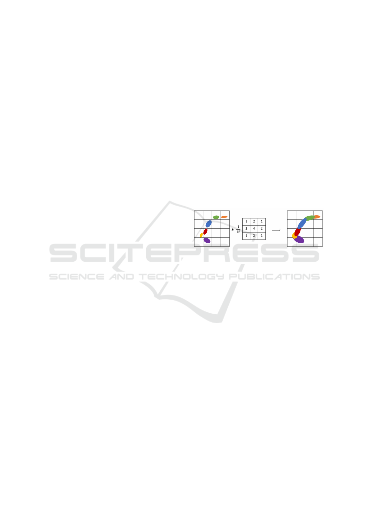
one iteration. The idea is to apply a smoothing kernel

to the NDT voxel grid, as illustrated in Figure 1. In

consequence, the distribution held by one voxel does

not only represent the distribution of the points within

this voxel any more, but the distribution of the points

in the surroundings of this voxel too.

Figure 1: Schematic representation of the smoothing step

for a 2D voxel grid to which a 3 × 3 sized Gaussian kernel

is applied. The distributions are represented by their conﬁ-

dence ellipses. The initial distributions (left) are blurred to

obtain the smoothed distributions (right).

When applying a smoothing kernel, the new ran-

dom variable X represented by aggregating the ran-

dom variables X

,...,X

with weighting coefﬁcients

,...w

is characterized by the mean and covariance

∑

i=1

(6)

∑

i=1

+ µ

) − µ

(7)

Each weight w

is also multiplied by the number

of points n

that fell into this voxel, before the sum of

weights is normalized to 1. This smoothing method

can be applied to the NDT map as a pre-processing

step. No additional storage costs are required, as after

construction only the smoothed distributions need to

be stored by each cell for the registration.

It might be noticed that the distributions are

obtained as a weighted sum of other distributions

(“mean of means”). Our experiments showed that it

produces better precision results than when taking di-

rectly a weighted sum of the points. Indeed, in the

Smoothed Normal Distribution Transform for Efﬁcient Point Cloud Registration During Space Rendezvous

921

latter case, more weight is artiﬁcially given to points

which happen to be close to the middle of a cell.

3.1.2 Covariance Matrix Regularization

Despite the smoothing, the covariance matrix of a dis-

tribution can still be singular, for instance for a set of

coplanar points. This happens quite often in practice,

as most scenes contain planar surfaces. To avoid such

cases, in probabilistic NDT each point is represented

by its own uncertainty distribution (Hong and Lee,

2017). Another possibility is to inﬂate the smallest

eigenvalues of singular or nearly singular covariance

matrices (Magnusson, 2009).

The proposed approach here is similar. For a pos-

itive semi-deﬁnite matrix C with maximal and mini-

mal eigenvalues λ

max

min

number is deﬁned as:

cond(C) =

max

(C)

min

(C)

∈ [1, +∞] (8)

Condition number regularization consists in mod-

ifying each covariance matrix C to satisfy the condi-

tion cond(C) ≤ κ, for κ > 1 (typically κ = 50). This

can be achieved by replacing C by C +δI, with δ given

by (Olive, 2022):

δ = max(0,

max

(C)− κλ

min

(C)

κ − 1

) (9)

3.2 Optimization Problem Formulation

3.2.1 Optimization on the so(3) Manifold

Euler angles are commonly used for representing the

rotation when using the NDT (Hong and Lee, 2017;

Lim et al., 2020). However, they come with the gim-

bal lock problem and necessary convention setting.

We make use of an alternative and convenient rep-

resentation. The rotation group SO(3) is a matrix lie

group, so that each element can be parametrized by

a 3-dimensional vector ω of the manifold. The cor-

responding rotation matrix is obtained by taking the

exponential of the cross-product matrix of ω

exp(ω

) = exp(





0 −ω

−ω





) (10)

In this way, the optimization problem in S =

SO(3)×R

can be reduced to a problem in R

×R

. The “boxplus” operator (Hertzberg et al., 2013)

is deﬁned to compute the new rotation and transla-

tion obtained after applying an increment from the

6D-manifold:

⊞ =



S × R

→ S

(R,t) ⊞ (ω, τ) = (exp(ω

)R, t + τ)

(11)

The Jacobian matrix of a transformation with pa-

rameters α = (R,t) evaluated at a 3D point z respec-

tively to the elements of the manifold ε = (ω, τ) yields

∂T (α ⊞ ε, z)

∂ε



ε=0





0 v

−v

1 0 0

−v

0 v

0 1 0

−v

0 0 0 1





(12)

where v = Rz. This Jacobian will be needed in the

next section.

3.2.2 Weighted Least Squares Optimization

For a simpler formulation of the optimization prob-

lem, we consider the relaxed problem where the non-

linear normal distribution representation has been

omitted. The residuals are

= T (α,z

) − µ

(13)

and the cost function is the sum of squared Maha-

lanobis distances:

s(α) =

∑

i=1

−1

(14)

where µ

, C

are the mean and covariance of the

distribution associated with point T (α,z

), and m

is the number of points from the source point cloud

which could be associated with a distribution. The

Jacobian of each residual is

∂T (α ⊞ ε, z

)

∂ε



ε=0

(15)

Stacking the Jacobians into the matrix J ∈ R

3m×6

the inverse covariances into the block-diagonal W ∈

3m×3m

, and the residuals into r ∈ R

, the increment

to perform according to the Gauss-Newton algorithm

is given by

W Jε = −J

W r (16)

After each iteration, the current estimate of the

transformation is updated according to α ← α ⊞ ε.

The optimization stops whenever one of the follow-

ing three conditions is reached:

• The maximum number of iterations is reached

• The norm of the increment ||ε|| is below a certain

threshold ε

min

• The number of points m

matched with the NDT

map does not increase, and the cost function (14)

increases.

VISAPP 2023 - 18th International Conference on Computer Vision Theory and Applications

922

3.3 Kd-Tree Adaptation

3.3.1 Kd-NDT Map

An NDT map is usually constructed using a regular

grid structure, typically an octree (Ulas¸ and Temeltas¸,

2013; Hong and Lee, 2017). Nevertheless, octrees

are not optimal because they map a lot of free space.

A strategy can be to store the cubical cells from the

regular grid subdivision into a kd-tree (Schulz et al.,

2018). Yet to the best of our knowledge, directly us-

ing a kd-tree with non-cubical cells for constructing

the NDT map has never been done. This is mainly

due to the fact that the distributions can be distorted

by the shape of kd-tree cells which can have a high

aspect ratio. However, this problem vanishes with the

smoothing method presented in the following Section

3.3.2.

The kd-tree is constructed as follows: At each sub-

division step, the new bounding box of all points is

computed. This is important for the efﬁciency of the

tree search at later steps. Then, the cell is split in

two children along its longest edge and in the mid-

dle. This ensures that the cells keep a good aspect ra-

tio. The subdivision stops once the kd-tree cells have

reached a certain size. The size of a kd-tree cell being

its longest edge l, if we want all cells to have an ap-

proximate cell size of r, the subdivision stops when-

ever the criteria l <

r is met. Consequently, all cells

have a size l ∈ [

r].

3.3.2 Smoothing of a kd-NDT Map

In the case of a kd-tree, the neighbouring cells to be

selected for performing the Gaussian smoothing step

are the ones which lie within a certain radius d

of the

center of the considered cell. Figure 2 illustrates this

idea.

Figure 2: Schematic representation of the smoothing step

in the case of a 2D kd-grid with non square cells. All the

cells within the radius are taken into account for computing

the smoothed distribution of the central cell. Here, only the

bottom right-cell is not considered because it lies too far

away.

Instead of using a discrete Gaussian kernel, a con-

tinuous Gaussian blur can be used. The contribution

of a distribution X

with n

points and mean µ

to the

smoothed distribution of a cell with center c is

∝ n

exp(−

||µ

− c||

2σ

) (17)

where σ is the standard deviation of the Gaussian

function. If r is the approximate resolution of the grid

map, in order for distributions located at a distance r

from the center to only have half the weight of distri-

butions located at the center, σ can be chosen as:

exp(−

2σ

) =

⇐⇒ σ =

2ln(2)

. (18)

In this way, a kd-tree cell of the smoothed NDT

tree holds the weighted distribution of all points lo-

cated in the inﬂuence sphere. Therefore, the actual

non-cubic but rectangular shape of the kd-tree cell

does not matter any more, and does not negatively

inﬂuence the shape of the distribution, what makes

the use of this kd-NDT map possible. The radius is

typically set to d

= 3σ to capture all signiﬁcant con-

tributions.

3.3.3 NDT Algorithm Adaptation

The algorithm described in Section 3.2.2 can be ap-

plied in the same way to kd-tree NDT maps. Each

point of the source cloud is associated to a distribu-

tion by performing a depth ﬁrst search. In our ex-

periments, this results in similar precision than exact

nearest cell search, and a speed-up by a factor approx-

imatively 1.5. Additionally, we deﬁne a maximum

point-to-cell distance d

p2c

. A point z is only associ-

ated with a distribution held by a cell with center c if

||z − c|| < d

p2c

4 RESULTS ON OUTDOOR

DATASETS

4.1 Datasets and Methodology

We compared the results of the algorithm on two

datasets of the Robotic 3D Scan Repository (N

uchter

and Lingemann, 2016). The ﬁrst dataset, Hanover 2,

was recorded with a Velodyne sensor at the campus

of the Leibniz University in Hanover. It contains 924

scans of each approximatively 13000 points (Figure

3). Initial pose estimates are provided and are pre-

cise at the order of a few degrees (< 5

◦

) and a few

Smoothed Normal Distribution Transform for Efﬁcient Point Cloud Registration During Space Rendezvous

923

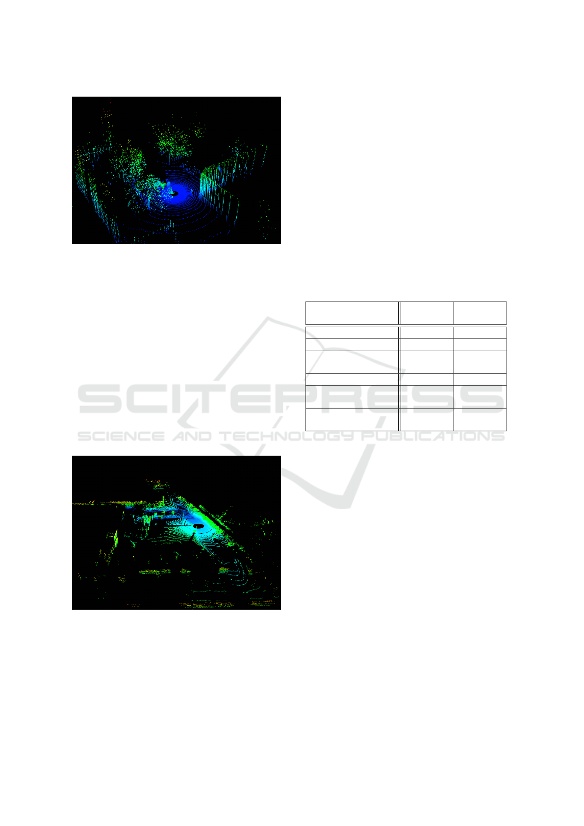
Figure 3: Scan 22 of the Hanover 2 dataset.

cm (∼ 10cm). Ground truth data is also available

uchter et al., 2010) starting from scan 22.

The second dataset contains 333 scans recorded

by a Velodyne scanner mounted on a car at the Univer-

sity of Koblenz-Landau. Each cloud contains about

100000 points (Figure 4). The initial pose estimates

are less precise than the previous ones (< 7

◦

in ro-

tation, and ∼ 1m in translation). Ground truth is

not available, however using the SLAM-6D algorithm

from the 3D toolkit (3DTK, 2022), we can generate

highly precise pose estimations which can be consid-

ered as ground truth for our problem. Simultaneous

localization and mapping (SLAM) is a global map-

ping method not suited for pairwise scan-registration.

Still, a core component of SLAM-6D is an ICP im-

plementation which we will use for comparison.

Figure 4: Scan 98 of the Koblenz University dataset.

We compared four algorithms for pairwise scan

registration, i.e. LiDAR odometry: The efﬁcient

state-of-the-art ICP implementation of the 3D toolkit

(3DTK, 2022) as reference, against our implementa-

tions of a classical NDT, the octree-based S-NDT and

the kd-tree based S-NDT. The implementations of the

“classical” NDT and the octree S-NDT only differ in

that the NDT map is being smoothed for the latter.

The algorithms were run on one core of an Intel Core

i7 CPU. It has to be noted that the ICP version of

3DTK is also optimized for multi threading and could

run on more cores.

4.2 Pairwise Scan Matching

The performance was evaluated by comparing the re-

sult of the registration of each pair of consecutive

scans with the expected result according to ground

truth. For all four algorithms, the scans were down-

sampled using a voxel grid ﬁlter in a pre-processing

step. The parameters used for the experiment are

summarized in Table 1.

Table 1: Parameters settings for the outdoor datasets.

Hanover 2

Koblenz

University

max iterations n

max

100 100

min increment ε

min

−5

voxel grid ﬁlter

resolution d

f ilter

10cm 20cm

(S-)NDT cell size r 50cm 150cm

ICP max point to

point distance d

p2p

75cm 150cm

S-NDT max point to

cell distance d

p2c

75cm 150cm

The results are presented on Figure 5 for the

Hanover 2 dataset and Figure 6 for Koblenz Univer-

sity. The ICP and S-NDT algorithms exhibit very

similar results for the translational and angular error

(Figures 5a, 5b, 6a, 6b). The precision of the classi-

cal NDT is close as well, but the angular errors are

slightly higher on the Hanover 2 dataset, and present

more outliers on the Koblenz University dataset. The

NDT and S-NDT implementations are signiﬁcantly

faster than the ICP, approximatively by a factor 4 (Fig-

ures 5c, 6c). They obtain a result in typically around

10 iterations, while the ICP converges within around

30 to 50 iterations (Figures 5d, 6d). For small point

clouds, the classical NDT is slightly faster than the

S-NDT, because then the smoothing step represents a

non-negligible part of the total processing time.

4.3 Robustness Evaluation

The robustness of an algorithm can be deﬁned in var-

ious ways: Sensitivity to noise, to initial conditions,

to different scenarios etc. In this section, we analyse

the sensitivity of the different algorithms to the pre-

cision of the initial estimate. Each algorithm being a

VISAPP 2023 - 18th International Conference on Computer Vision Theory and Applications

924

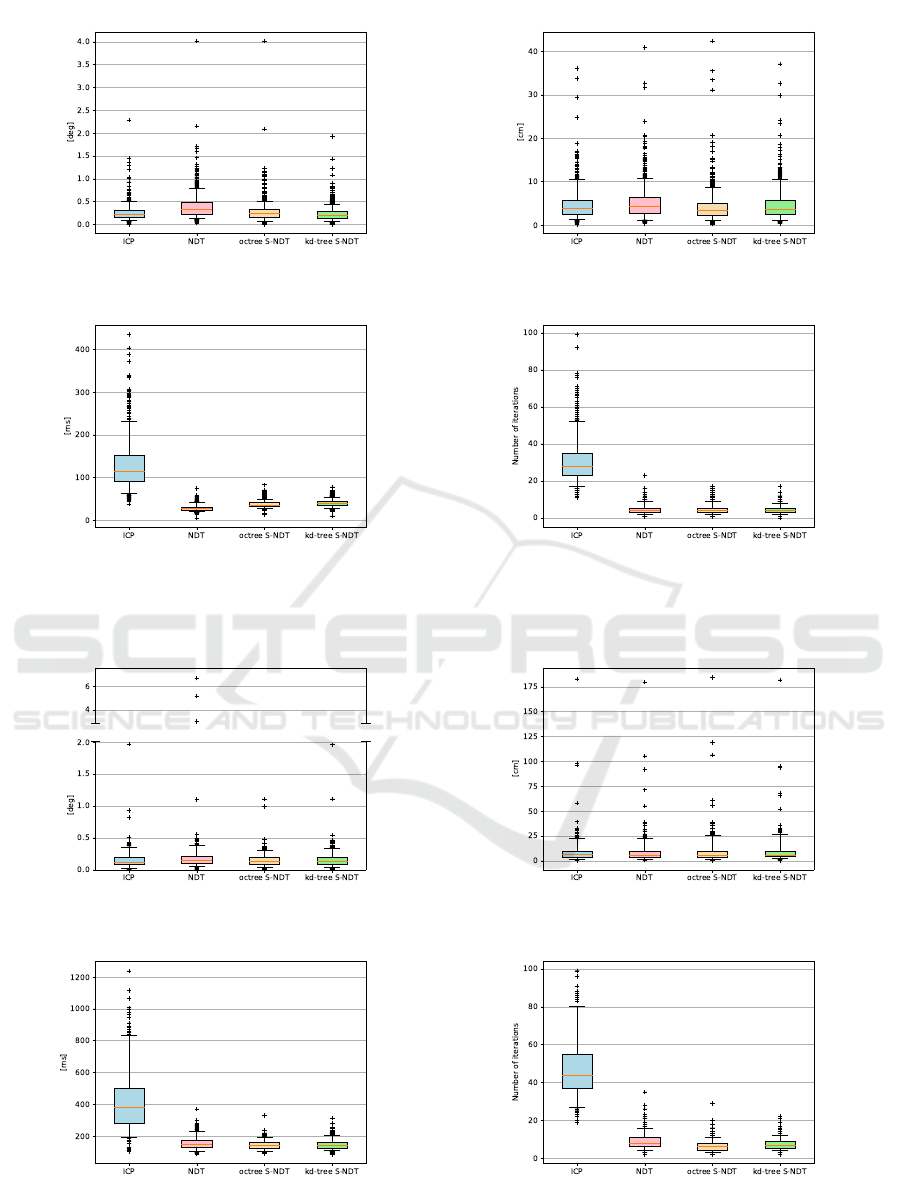
(a) Angular errors. (b) Translational errors.

Figure 5: Distribution of the errors and key characteristics of each algorithm, when performing pairwise scan registration

from scan 22 to 923 of the Hanover 2 dataset.

(a) Angular errors. (b) Translational errors.

Figure 6: Distribution of the errors and key characteristics of each algorithm, when performing pairwise scan registration

from scan 1 to 328 of the Koblenz university dataset.

Smoothed Normal Distribution Transform for Efﬁcient Point Cloud Registration During Space Rendezvous

925

local optimization method, its convergence basin can

be seen as the set of initial translational and angular

errors for which the algorithm converges.

The convergence basin is estimated using a

Monte-Carlo method. The 2D space of initial trans-

lation and angular errors is divided into discrete data

points. For each of these points, the probability that

each algorithm converges is estimated. The estima-

tion is the average of successes observed when repeat-

ing 50 times the following random experiment: Select

two consecutive scans at random, and starting from

the perfect alignment, rotate and translate one scan

along a random axis and a random direction in order

to reach the desired angular and translational errors.

Afterwards start the algorithm from this initial pose,

and evaluate the result.

The criteria for deﬁning if a method was suc-

cessful is based on the results obtained on the two

datasets (Figures 5 and 6): For Hanover 2, a registra-

tion is considered to be successful if the error is below

1.5deg and 30cm. For Koblenz University, the limits

were set to 1.2deg and 75cm. The heat maps repre-

senting the estimated convergence basins of each al-

gorithm for both datasets following this method are

presented on Figures 7 and 8. On the Hanover 2

dataset, the ICP algorithm shows to be the most ro-

bust, followed closely by the kd-tree S-NDT. The oc-

tree S-NDT turns out to have poorer convergence re-

sults, but they are still better than the classical NDT.

On the Koblenz university dataset however, both S-

NDT implementations demonstrate better robustness

than the ICP and NDT.

4.4 Discussion

If all four algorithms are suited for precise scan

matching, the speed advantage of the NDT and S-

NDT versions makes them particularly interesting for

real-time applications. Nevertheless, if the ICP is

such a popular algorithm, it is also because of its

robustness. The NDT shows to have a smaller con-

vergence basin compared to the ICP. The challenge

was to develop an algorithm proﬁting from the speed-

up potential of the NDT formulation, while achiev-

ing similar robustness as the ICP. The experiments

demonstrate that the smoothing step of the S-NDT

increases the convergence basin of the algorithm. If

the octree S-NDT formulation still has poorer conver-

gence results then the ICP on the Hanover 2 dataset,

the kd-tree version shows consistently good results on

both datasets.

The performance of the ICP in terms of robustness

differs depending on the considered dataset (Figures

7a and 8a). A possible explanation resides in the fact

that the Hanover 2 dataset represents rather small out-

door scenes, while Koblenz University contains large

scale scans with considerably more points (see Fig-

ures 3 and 4 for comparison). The ICP being an algo-

rithm that considers every point to point association,

a hypothesis is that it fails to get the bigger picture

on such scans, resulting in it being stuck in a local

optimum. In contrast, the NDT algorithm computes

voxel-wise distributions for a more coarse representa-

tion of the point cloud.

The main advantage of the kd-tree formulation is

the ﬂexibility in the implementation. Speciﬁcally, be-

ing able to set a maximum point-to-cell distance for

considering or rejecting associations enables to widen

the attraction domain of a distribution, and thus the

overall algorithm’s convergence basin. Of the four

methods, the kd-tree S-NDT appears to be the most

suited method for precise, reliable and efﬁcient point

cloud registration.

5 APPLICATION TO

SPACECRAFT POSE

TRACKING

5.1 Testing Environment

5.1.1 European Proximity Operations Simulator

The European Proximity Operations Simulator or

EPOS (Benninghoff et al., 2017), is a high-ﬁdelity

hardware in the loop simulator for spacecraft proxim-

ity operations, maintained by the German Space Op-

erations Center. This simulator can be used to gen-

erate test data for the context of LiDAR pose track-

ing of an uncooperative satellite during autonomous

space rendezvous.

The facility consists of two robotic arms carry-

ing a load (Figure 9), which can move with 6 de-

grees of freedom. The robot on the left on the pic-

ture represents the active and controlled satellite, also

called servicer satellite. It has a Livox-Mid40 Li-

DAR installed on its plate. Additionally, this robot is

mounted on a 25m long linear rail to simulate transla-

tional movement. The second robot holds a mock-up

of the target satellite at scale 1:1, which is made of re-

alistic materials (solar panels, golden MLI sheets). To

reproduce space dynamics, the facility is coupled to a

dynamics simulator. A guidance and control system

is used to follow a desired rendezvous trajectory.

For estimating the relative pose of the target satel-

lite, a navigation ﬁlter uses as input the result of the

tracking of multiple sensors such as an RGB camera,

VISAPP 2023 - 18th International Conference on Computer Vision Theory and Applications

926

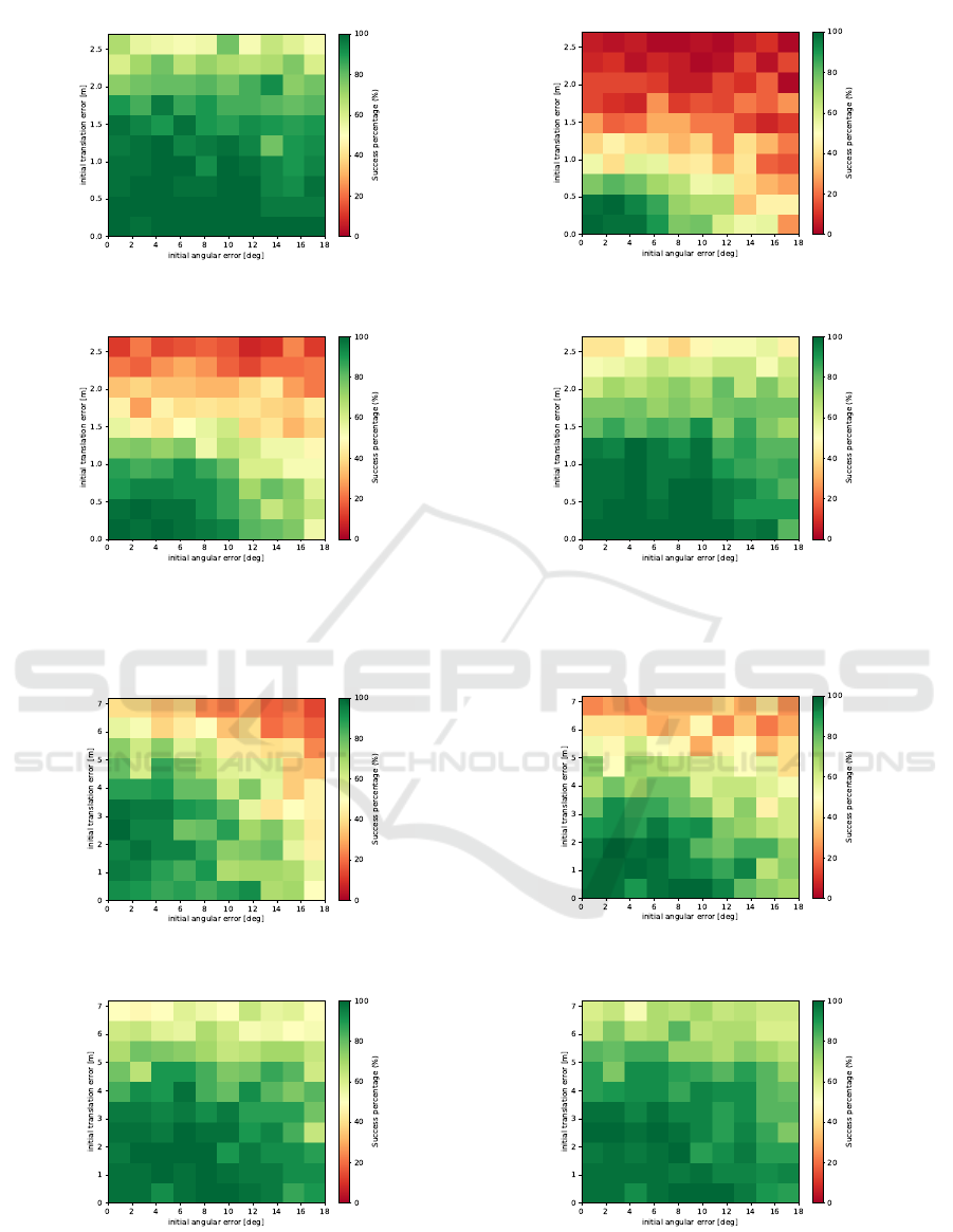
(a) Convergence basin for the ICP.

(b) Convergence basin for the classical NDT.

Figure 7: Heat maps representing the convergence basin of each algorithm on the Hanover 2 dataset. Scans were selected at

random following a Monte-Carlo method. The maximum registration error for deﬁning success was set to 1.5deg and 30cm.

(a) Convergence basin for the ICP.

(b) Convergence basin for the classical NDT.

Figure 8: Heat maps representing the convergence basin of each algorithm on the Koblenz university dataset. Scans were

selected at random following a Monte-Carlo method. The maximum registration error for deﬁning success was set to 1.2deg

and 75cm.

Smoothed Normal Distribution Transform for Efﬁcient Point Cloud Registration During Space Rendezvous

927

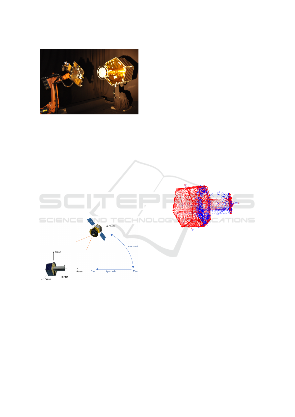
Figure 9: Picture of the EPOS facility robots.

PMD camera and a LiDAR (Frei et al., 2022). Ulti-

mately, the goal of the LiDAR pose estimation is to

provide input for this navigation ﬁlter on-line. How-

ever, for this experiment, the data was ﬁrst collected

separately and the tracking was done off-line.

In order to obtain realistic point clouds representa-

tive of space conditions, the points which correspond

to the robotic arm or the background of the testing fa-

cility are cut out automatically. Because of the quality

of the sensor and the reﬂecting materials on the satel-

lite such as the golden MLI sheets, the point clouds

are noisy and distorted, as can be observed on Figure

11.

5.1.2 Rendezvous Scenario

Figure 10: Schematic representation of the rendezvous tra-

jectory.

The LiDAR data was collected during a ren-

dezvous simulation at EPOS with following scenario,

schematically represented on Figure 10: First, the ser-

vicer satellite performs a ﬂy-around of the tumbling

target satellite at a steady distance of 15m in order to

inspect it from different angles. Then, it ﬂies back to

its initial point and the approach is started. The ﬁrst

approach part, until 8m, is performed with a velocity

of 2cm/s, and the ﬁnal approach to 3m with a veloc-

ity of 1cm/s. Throughout the whole experiment of

around 20 minutes, the target satellite spins around its

main axis (x

LVLH

) at a rate of 1deg/s.

During the rendezvous, the LiDAR captures point

clouds with an adaptive frequency, such that every

point cloud contains around 10000 points. Therefore,

at 15m, the frequency of the LiDAR is of around 1Hz,

while it can go up to 4Hz for the shortest ranges in this

experiment (3m). In total, the dataset for this trajec-

tory contains 1644 point clouds.

5.2 Pose Tracking

5.2.1 Strategy

In this scenario, a geometrical model of the target

satellite is known in the beforehand. Thus we do not

one, but perform registration of each scan respectively

to a model point cloud of the target as shown in Figure

11. The tracking is performed with the kd-tree based

S-NDT algorithm, and the smoothed NDT map of the

model point cloud only has to be computed once for

the whole experiment.

Figure 11: Point cloud captured by the LiDAR at EPOS

(blue) superimposed with a model point cloud of the target

(red). The captured point cloud is noisy and distorted due

to reﬂections on the golden MLI sheets.

For every new incoming point cloud, the result of

the previous registration step is used as initial esti-

mation. Still, for the very ﬁrst point cloud, an initial

guess has to be formulated. This would be the task of

a dedicated pose initialization algorithm. In the con-

text of this work, such an algorithm was not devel-

oped. The pose initialization is assumed to be perfect

and is obtained using the ground truth available at the

EPOS facility.

5.3 Results and Discussion

The experiment was run on one core of an Intel Core

i7 CPU, with following parameters for the S-NDT:

max

= 50, ε

min

= 10

−3

, d

f ilter

= 2cm

r = 7.5cm, d

p2c

= 7.5cm

(19)

VISAPP 2023 - 18th International Conference on Computer Vision Theory and Applications

928

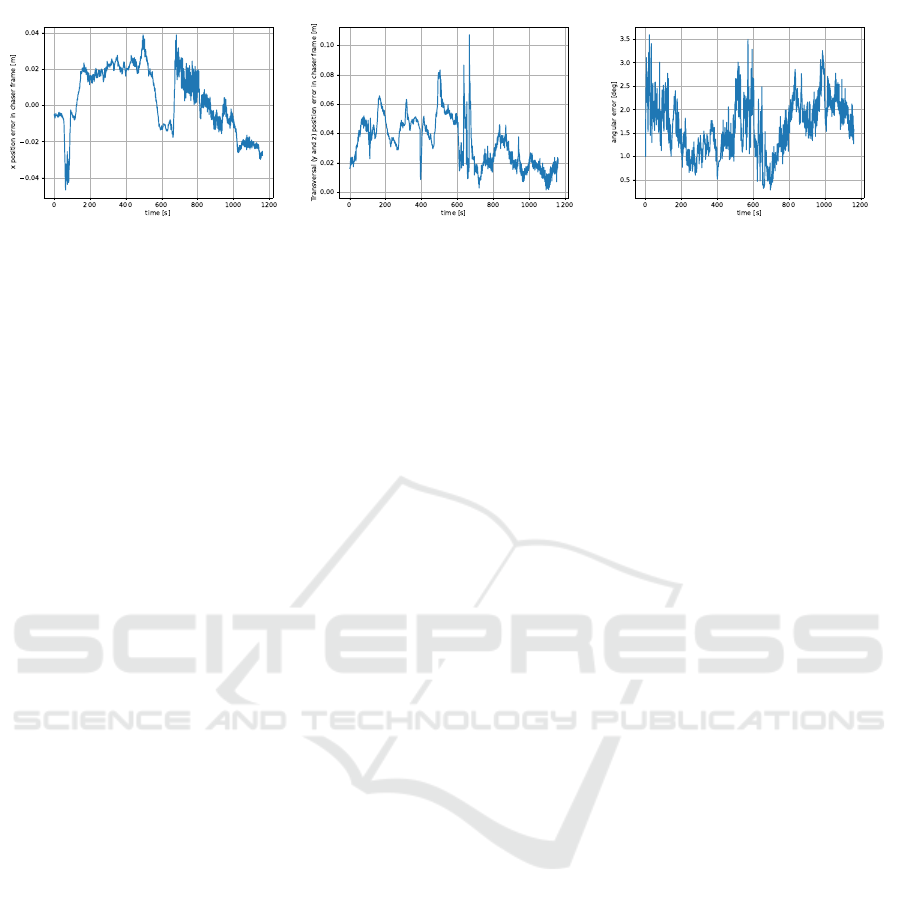
(a) Radial position error (along the Li-

DAR optical axis).

(b) Transversal position error. (c) Angular error.

Figure 12: Translational and angular errors of the tracking of the spacecraft’s center of mass and orientation when compared

to the ground truth at EPOS. The oscillation of the chaser when initiating the approach at t = 670s leads to the biggest tracking

error.

The results are presented on Figure 12. The ﬁrst

phase of the ﬂight is the ﬂy-around, and the approach

from 15m to 3m starts at t = 670s. The position of

the target satellite’s center of mass is tracked. Both

the frontal (along the x axis) and the transversal (y

and z axes) errors are below 11cm throughout the ex-

periment. When getting closer to the target satellite,

this error further decreases to a few cm. The angular

error of the spacecraft’s estimated orientation is below

3.6deg.

The translational and angular errors of the track-

ing are sufﬁcient for performing an approach up to a

distance of a few meters of the target. Nevertheless,

some improvement could probably be obtained by us-

ing a more accurate 3D model of the target satellite

than the current one. The LiDAR’s frame rate is also

an important parameter. If it is too high, the captured

point cloud is not dense enough, but if it is too low,

the measurement is delayed and might be distorted

(motion blur). This motivated the current choice of

an adaptive frame rate ensuring that all point clouds

are equally dense. Nevertheless, when manoeuvres

are performed, the delay and motion blur effects can

already be observed and lead to loss of precision in

the tracking, for instance at t = 670s.

The average processing time for down-sampling

a point cloud and performing the S-NDT registration

was of 18 milliseconds. This demonstrates that the al-

gorithm is suited for real-time tracking requirements.

However, currently the processing was done on a stan-

dard computer, and further work might include testing

the algorithm on space-representative hardware.

6 CONCLUSIONS

In this paper, we proposed a modiﬁed S-NDT algo-

rithm in order to reach better efﬁciency for real-time

tracking applications. We introduced a novel smooth-

ing method of the NDT map based on Gaussian blur-

ring. Combined with a kd-tree representation of the

map, it leads to a better robustness while maintain-

ing the algorithm’s speed. The S-NDT was tested in

different contexts. When compared to ICP on out-

door datasets from the automotive domain, it is sig-

niﬁcantly faster while achieving the same accuracy.

The experiments show that it is also a fast, precise and

reliable registration method for satellite pose tracking

during autonomous space rendezvous.

Nevertheless, the method remains a local opti-

mization method, which has to be coupled with a

global optimization procedure in order for a system

to navigate autonomously. In the context of au-

tonomous driving, a loop detection procedure such as

SLAM would be required to detect already scanned

environments and correct the accumulated drift. For

spacecraft pose tracking, a global pose initialization

method is needed to initiate the tracking, and will be

the subject of future work. Other potential limitations

could arise when tracking faster objects. If the rela-

tive movements in the context of satellite rendezvous

are rather slow, with faster dynamics, effects such as

motion blur could arise and lead to a distortion of the

point clouds which would have to be taken into ac-

count.

REFERENCES

3DTK (2022). The 3D toolkit. [Online]. Available: https:

//slam6d.sourceforge.io/index.html.

Benninghoff, H., Rems, F., Risse, E.-A., and Mietner, C.

(2017). European proximity operations simulator 2.0

(epos)-a robotic-based rendezvous and docking simu-

lator. Journal of large-scale research facilities JLSRF.

Besl, P. J. and McKay, N. D. (1992). Method for regis-

tration of 3-d shapes. In Sensor fusion IV: control

paradigms and data structures, volume 1611, pages

586–606. Spie.

Smoothed Normal Distribution Transform for Efﬁcient Point Cloud Registration During Space Rendezvous

929

Biber, P. and Straßer, W. (2003). The normal distribu-

tions transform: A new approach to laser scan match-

ing. In Proceedings 2003 IEEE/RSJ International

Conference on Intelligent Robots and Systems (IROS

2003)(Cat. No. 03CH37453), volume 3, pages 2743–

2748. IEEE.

Chetverikov, D., Svirko, D., Stepanov, D., and Krsek, P.

(2002). The trimmed iterative closest point algorithm.

In 2002 International Conference on Pattern Recogni-

tion, volume 3, pages 545–548. IEEE.

Das, A., Servos, J., and Waslander, S. L. (2013). 3d scan

registration using the normal distributions transform

with ground segmentation and point cloud clustering.

In 2013 IEEE international conference on robotics

and automation, pages 2207–2212. IEEE.

Droeschel, D., St

uckler, J., and Behnke, S. (2014). Local

multi-resolution representation for 6d motion estima-

tion and mapping with a continuously rotating 3d laser

scanner. In 2014 IEEE International Conference on

Robotics and Automation (ICRA), pages 5221–5226.

IEEE.

Frei, H., Burri, M., Rems, F., and Risse, E.-A. (2022). A

robust navigation ﬁlter fusing delayed measurements

from multiple sensors and its application to spacecraft

rendezvous. Advances of Space Research, Special Is-

sue on Space Environment Management and Space

Sustainability.

Hertzberg, C., Wagner, R., Frese, U., and Schr

oder, L.

(2013). Integrating generic sensor fusion algorithms

with sound state representations through encapsula-

tion of manifolds. Information Fusion, 14(1):57–77.

Hong, H. and Lee, B. H. (2017). Probabilistic normal distri-

butions transform representation for accurate 3d point

cloud registration. In 2017 IEEE/RSJ International

Conference on Intelligent Robots and Systems (IROS),

pages 3333–3338. IEEE.

Koide, K., Yokozuka, M., Oishi, S., and Banno, A. (2021).

Voxelized gicp for fast and accurate 3d point cloud

registration. In 2021 IEEE International Conference

on Robotics and Automation (ICRA), pages 11054–

11059. IEEE.

Lim, H., Hwang, S., Shin, S., and Myung, H. (2020). Nor-

mal distributions transform is enough: Real-time 3d

scan matching for pose correction of mobile robot un-

der large odometry uncertainties. In 2020 20th Inter-

national Conference on Control, Automation and Sys-

tems (ICCAS), pages 1155–1161. IEEE.

Magnusson, M. (2009). The three-dimensional normal-

distributions transform: an efﬁcient representation

for registration, surface analysis, and loop detection.

PhD thesis,

Orebro universitet. Pages 58–65.

Magnusson, M., Nuchter, A., Lorken, C., Lilienthal, A. J.,

and Hertzberg, J. (2009). Evaluation of 3d registration

reliability and speed-a comparison of icp and ndt. In

2009 IEEE International Conference on Robotics and

Automation, pages 3907–3912. IEEE.

uchter, A., Elseberg, J., Schneider, P., and Paulus, D.

(2010). Study of parameterizations for the rigid

body transformations of the scan registration prob-

lem. Computer Vision and Image Understanding,

114(8):963–980.

uchter, A. and Lingemann, K. (2016). Robotic 3D scan

repository. [Online]. Available: http://kos.informatik.

uni-osnabrueck.de/3Dscans/.

Olive, D. (2022). Prediction and statistical learning. page

344, preprint M-02-006. [Online]. Available: http://

lagrange.math.siu.edu/Olive/slearnbk.htm.

Pang, S., Kent, D., Cai, X., Al-Qassab, H., Morris, D., and

Radha, H. (2018). 3d scan registration based localiza-

tion for autonomous vehicles-a comparison of ndt and

icp under realistic conditions. In 2018 IEEE 88th ve-

hicular technology conference (VTC-Fall), pages 1–5.

IEEE.

Pyrak, M. and Anderson, J. (2022). Performance of

northrop grumman’s mission extension vehicle (mev)

rpo imagers at geo. In Autonomous Systems: Sen-

sors, Processing and Security for Ground, Air, Sea

and Space Vehicles and Infrastructure 2022, volume

12115, pages 64–82. SPIE.

Schulz, C., Hanten, R., and Zell, A. (2018). Efﬁcient map

representations for multi-dimensional normal distri-

butions transforms. In 2018 IEEE/RSJ International

Conference on Intelligent Robots and Systems (IROS),

pages 2679–2686. IEEE.

Segal, A., Haehnel, D., and Thrun, S. (2009). Generalized-

icp. In Robotics: science and systems, volume 2, page

435. Seattle, WA.

Stoyanov, T., Magnusson, M., and Lilienthal, A. J. (2012).

Point set registration through minimization of the l 2

distance between 3d-ndt models. In 2012 IEEE In-

ternational Conference on Robotics and Automation,

pages 5196–5201. IEEE.

Takeuchi, E. and Tsubouchi, T. (2006). A 3-d scan matching

using improved 3-d normal distributions transform for

mobile robotic mapping. In 2006 IEEE/RSJ Interna-

tional Conference on Intelligent Robots and Systems,

pages 3068–3073. IEEE.

Ulas¸, C. and Temeltas¸, H. (2013). 3d multi-layered nor-

mal distribution transform for fast and long range scan

matching. Journal of Intelligent & Robotic Systems,

71(1):85–108.

VISAPP 2023 - 18th International Conference on Computer Vision Theory and Applications

930