Optimal Activation Function for Anisotropic BRDF Modeling

Stanislav Mike

and Michal Haindl

Institute of Information Theory and Automation of the ASCR, Pod Vod

arenskou v

ı 4, Prague, Czechia

Keywords:

Anisotropic BRDF Models, Neural Network, Activation Function, BTF.

Abstract:

We present simple and fast neural anisotropic Bidirectional Reﬂectance Distribution Function (NN-BRDF)

efﬁcient models, capable of accurately estimating unmeasured combinations of illumination and viewing an-

gles from sparse Bidirectional Texture Function (BTF) measurement of neighboring points in the illumina-

tion/viewing hemisphere. Our models are optimized for the best-performing activation function from nineteen

widely used nonlinear functions and can be directly used in rendering. We demonstrate that the activation

function signiﬁcantly inﬂuences the modeling precision. The models enable us to reach signiﬁcant time and

cost-saving in not trivial and costly BTF measurements while maintaining acceptably low modeling error. The

presented models learn well, even from only three percent of the original BTF measurements, and we can

prove this by precise evaluation of the modeling error, which is smaller than the errors of alternative analytical

BRDF models.

1 INTRODUCTION

Visual scenes are predominantly represented with

shapes and materials, and thus their recognition re-

quires them to represent these properties realistically.

Unfortunately, the surface material appearance con-

siderably changes under variable observation condi-

tions, which signiﬁcantly negatively affects its au-

tomatic, reliable recognition in numerous artiﬁcial

intelligence applications. As a consequence, most

material recognition attempts apply unnaturally re-

stricted observation conditions (Varma and Zisser-

man, 2009; Bell et al., 2015; Gibert et al., 2015).

A surface material point representation that respects

its appearance changes due to illumination and view-

ing conditions variations are the Bidirectional Re-

ﬂectance Distribution Function (BRDF). A multi-

dimensional visual texture is appropriate for a spa-

tial surface reﬂectance function model. The best mea-

surable representation is the seven-dimensional Bidi-

rectional Texture Function (BTF) (Haindl and Filip,

2013). BTF can be simultaneously measured, even if

it is not a trivial task, and modeled using state-of-the-

art measurement devices and computers as well as the

most advanced mathematical models of visual data.

Features derived from such multi-dimensional BTF

data models are information-preserving in the sense

https://orcid.org/0000-0001-5741-8940

https://orcid.org/0000-0001-8159-3685

that they can be used to synthesize data spaces closely

resembling the original measurement data space.

The ﬁve-dimensional BRDF model obeys thirteen

simplifying assumptions (Haindl and Filip, 2013)

from the general reﬂectance model, among them non-

negativity, energy conservation, and the Helmholtz

reciprocity (von Helmholtz, 1867). Hence, the BRDF

model depends only on ﬁve variables:

BRDF

= BRDF(λ,θ

,ϕ

,θ

,ϕ

) , (1)

where Y is a multispectral pixel, λ the spectral vari-

able, θ

,ϕ

elevation and azimuthal illumination an-

gles, and θ

,ϕ

are elevation and azimuthal viewing

angles. Isotropic BRDF models represent materials

whose reﬂections do not depend on the orientation of

the azimuthal angles but only on their difference.

Several analytical isotropic (Minnaert, 1941;

Phong, 1975; Blinn, 1977; Cook and Torrance, 1982;

Strauss, 1990; Oren and Nayar, 1994; Ngan et al.,

2005) as well as anisotropic (Torrance and Spar-

row, 1966; Ward, 1992; Schlick, 1993; Lafortune

et al., 1997; Ashikhmin and Shirley, 2000; Ragheb

and Hancock, 2008; Dahlan and Hancock, 2016)

BRDF models were proposed. The problem of recon-

structing a measured isotropic BRDF from a limited

number of BRDF-measured samples is addressed in

(Nielsen et al., 2015). Another data-driven acquisi-

tion method of isotropic BRDF from two images was

presented in (Xu et al., 2016). These models use only

isolated pixel-based BRDF measurements and thus

162

Mikeš, S. and Haindl, M.

Optimal Activation Function for Anisotropic BRDF Modeling.

DOI: 10.5220/0011616200003417

In Proceedings of the 18th International Joint Conference on Computer Vision, Imaging and Computer Graphics Theory and Applications (VISIGRAPP 2023) - Volume 1: GRAPP, pages

162-169

ISBN: 978-989-758-634-7; ISSN: 2184-4321

 2023 by SCITEPRESS – Science and Technology Publications, Lda. Under CC license (CC BY-NC-ND 4.0)

reduce and less precise information than our proposed

model, which learns from more informative and richer

BTF data.

A neural BRDF model for joint estimation of re-

ﬂectance and natural illumination from a single im-

age of an object of known geometry was suggested

in (Chen et al., 2021). Another neural network-

based representation of BRDF data that enables the

importance sampling of BRDFs was presented in

(Sztrajman et al., 2021), but they use artifact-prone

non-smooth activation function and less informative

BRDF measurements.

Neural BRDF representation (Zheng et al., 2021)

expresses BRDFs as continuous functions and al-

lows importance sampling, but its extrapolation is

poor. Neural BRDF model (Fan et al., 2021), which

considers only isotropic materials, was applied to

spatially-varying bidirectional reﬂectance distribution

functions.

The isotropic BRDF models cannot represent

materials with an anisotropic appearance faithfully

(Ngan et al., 2005). However, most materials have an

anisotropic appearance. Thus the isotropy is a severe

limitation. Hence there is a need to develop novel,

fully anisotropic BRDF models. The isotropic BRDF

is a particular case of general anisotropic BRDF. Thus

the presented model can faithfully model also any

isotropic BRDF.

We propose a novel anisotropic deep neural net-

based model for BRDF, which reliably learns BRDF

model parameters from sparse BTF measurements.

The NN model has numerous parameters, including

network topology, initialization, optimizer, learning

rate, loss function or angular representation, and oth-

ers. Simultaneous optimization of all these free pa-

rameters is time-demanding. Thus, we have opti-

mized the network topology and, subsequently, the

activation function. We show that the activation func-

tion signiﬁcantly inﬂuences the modeling precision.

Our contribution is a novel anisotropic deep neural

net-based BRDF model, model learning from more

informative BTF measurements, and optimization of

the activation function.

For our analysis in this paper, we take advantage

of unique anisotropic UTIA BTF visual material mea-

surements (Haindl et al., 2012; Haindl et al., 2015)

detailed in the following section, and we can provide

an accurate evaluation of modeling error.

2 BRDF MEASUREMENTS

The UTIA BTF database was measured using a high-

precision robotic gonioreﬂectometer (Haindl et al.,

Table 1: The number of used samples in training subsets.

v•-i• ia is

va 81 × 81 100% (6561) 81 × 14 17% (1134)

vs 81 × 14 17% (1134) 14 × 14 3% (196)

spruce

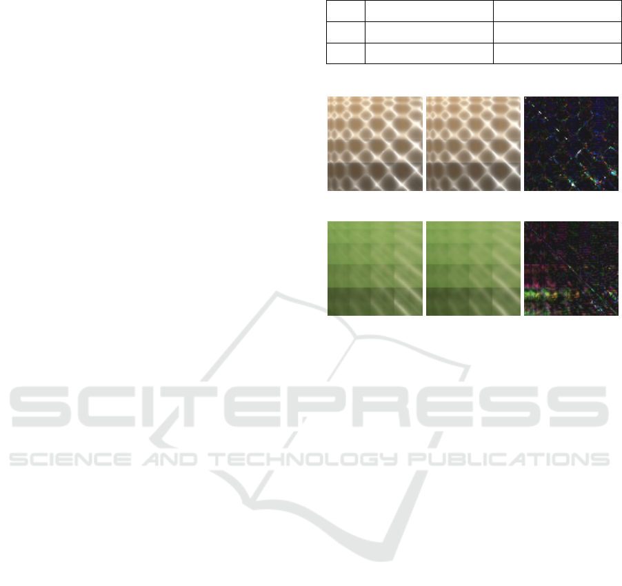
measured BRDF estimated BRDF BRDF difference

green cloth

Figure 1: Spruce and cloth examples of the UTIA BTF

database modeling results (models 15–30–20 with Soft-

Sign, va-ia). Error difference images are enhanced to be-

come visible.

2012). The setup consists of independently controlled

arms with a camera and light. Its parameters, such as

angular precision of 0.03 degrees, the spatial resolu-

tion of 1000 DPI, or selective spatial measurement,

classify this gonioreﬂectometer as a state-of-the-art

device. The typical resolution of the area of interest is

around 2000 × 2000 pixels, sample size 7 × 7 [cm],

sensor distance ≈ 2 [m] with the ﬁeld of view an-

gle 8.25

◦

and each of them is represented using at

least a 16-bit ﬂoating-point value for a reasonable

representation of high-dynamic-range visual informa-

tion. The illumination source is eleven LED arrays,

each having ﬂux 280 lm at 0.7 A, spectral wavelength

450 − 700 [nm], and have its optics. The memory

requirements for storage of a single material sample

amount to 360 gigabytes per color channel but can be

much more for a more precise spectral measurement.

2.1 Measured BRDF

We measured each material sample in 81 viewing po-

sitions n

and 81 illumination positions n

resulting

in 6561 images per sample (4 terabytes of data). We

compute each BRDF value from its corresponding an-

gular BTF measurement. These measured BRDF val-

ues, illustrated for spruce and green cloth in Fig. 1, we

further use as the ground truth for the neural BRDF

Optimal Activation Function for Anisotropic BRDF Modeling

163

angular input

(2 × 3)

hidden

)

hidden

)

hidden

)

RGB output

(3)

Figure 2: Neural network model.

model evaluation.

3 NEURAL NETWORK BRDF

MODELS

We have experimentally veriﬁed neural models capa-

ble of accurately approximating unmeasured combi-

nations of the illumination and viewing angles in the

anisotropic BRDF space. Using cross-validation, the

proposed model was selected from a set of simple

deep neural models optimizing the BRDF modeling

error Eq. (3). These simple models offer good mod-

eling precision while simultaneously avoiding huge

training set requirements, thus there is no need to

use any complex state-of-the-art neural models. Our

model (Fig. 2) starts with the view and illumination

angles representation vector. Then several fully con-

nected layers follow. The number of neurons in the

hidden layers is 15–30–20, or 3–6–4 for a simpler

model. The last (output) layer has three neurons cor-

responding to the RGB color. Except for the last

layer, all neurons have one of the twenty selected ac-

tivation functions (Fig. 3), and the last layer is lin-

ear. We implemented the neural network in the Ten-

sorﬂow framework and designed it in a parallel way

(81 × 81) to speed up training and prediction compu-

tations. The overall number of trainable parameters is

1268, or 88 for the simpler model. We used Glorot

uniform initialization of weights, Adamax optimizer

with a learning rate of 0.0025 and mean absolute er-

ror as the loss function. The models were trained for

500 epochs, and the times (Tab. 3–right) are measured

on Tesla P100 / 16GB.

3.1 Angle Representation

The view and illumintation directions are described

by spherical angles (θ

,φ

), (θ

,φ

), where elevation

/ polar angle θ

•

∈ ⟨0, 90) and azimuthal angle φ

•

∈

⟨0,360). We tested six different angle representa-

tions (e.g., Rusinkiewicz parametrization) for the in-

put vector in our neural network model. The angle

vectors are designed to overcome the discontinuity of

azimuthal angle; the proposed formula for xyz repre-

sentation follows:



sin(

θπ

180

)·sin(

φπ

180

),sin(

θπ

180

)·cos(

φπ

180

),cos(

θπ

180

)



Our estimation error results suggest the preferability

to use xyz for angle vector representation.

3.2 Activation Functions

We have selected the majority of published activa-

tion functions while excluding only some of their mi-

nor modiﬁcations. We have veriﬁed our assumption

that non-smooth activation functions (Shamir et al.,

2020) such as the Heaviside function, Piece-wise lin-

ear, Signum, ReLu, rReLu, SELU, HardTanh, Hard-

Shrink, SoftMax, SoftShrink, HardSigmoid are prone

to create visual artifacts in areas around their non-

smooth gradients. While authors (Shamir et al., 2020)

searched for the average individual per-example class

prediction difference over a set of models that are

conﬁgured, trained, and supposed to be identical over

some validation dataset, we aim to achieve modeling

accuracy robustness to different training sets while

simultaneously avoiding erroneous visual artifacts.

Among the smooth activation functions (Shamir et al.,

2020), ELU, Exponential, GELU, LiSHT, Mish, Sig-

moid, SoftSign, Swish, Tanh, Snake, SoftPlus, and

TanhShrink are searched for the most robust function

which guarantees the best approximation accuracy for

the wide range of sparse BTF measurements.

3.3 Training Subsets

Fig. 4 shows spherical sampling over angular space.

Two different angular subsets (all,sixth) are used to

create learning sets for the neural network model. The

training sets consist of texture patches with differ-

ent views and illumination directions. Tab. 1 com-

prises the combinations of view and illumination

subsets with the corresponding number of training

patches and their relative size (concerning full mea-

sured space, i.e., 6561 patches).

4 RESULTS

The proposed BRDF model was trained using various

subsets of the fully measured BTF texture space. For

the experiments, we tested six wood veneers and nine

other UTIA BTF material database materials. Two

of them, the spruce veneer and green cloth, are il-

lustrated here. The other thirteen materials conﬁrm

our conclusions. We tested four subset combinations

GRAPP 2023 - 18th International Conference on Computer Graphics Theory and Applications

164

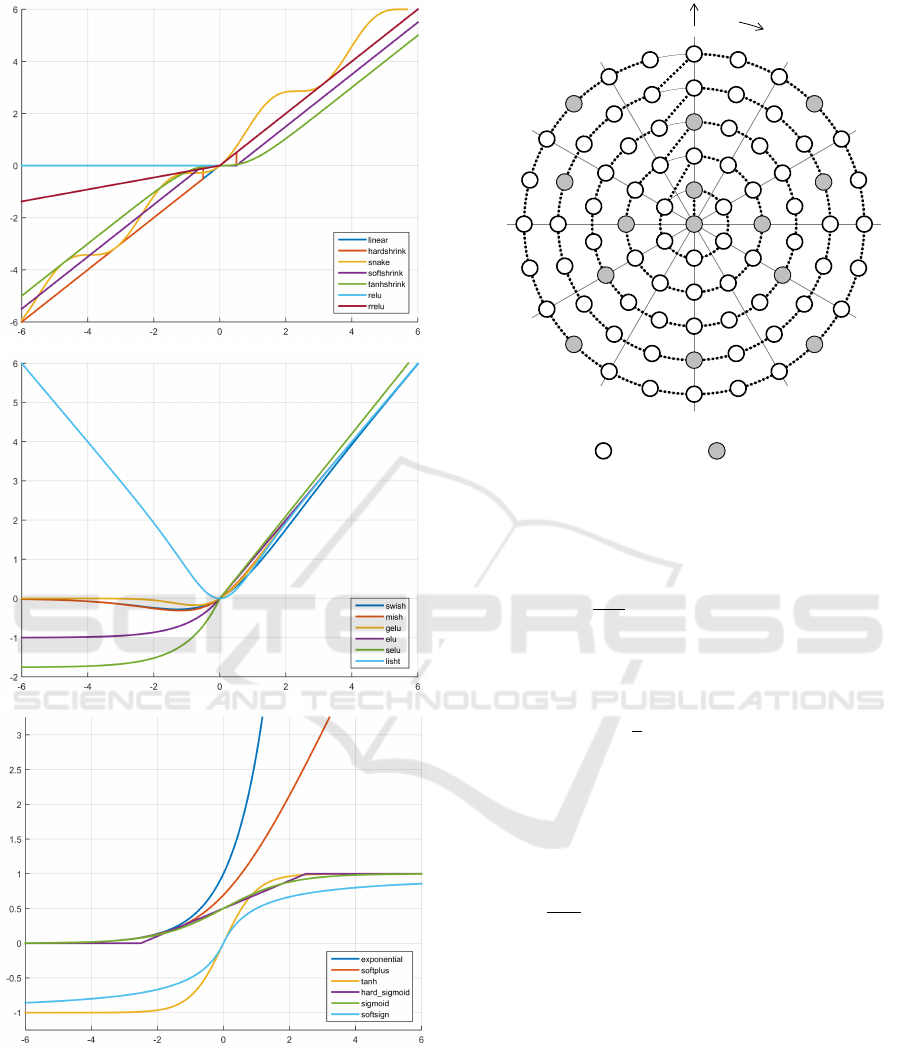
Figure 3: Nineteen of the tested activation functions (top –

Linear, HardShrink, Snake, SoftShrink, TanhShrink, ReLu,

rReLu; middle – Swish, Mish, GELU, ELU, SELU, LiSHT;

bottom – Exponential, SoftPlus, Tanh, HardSigmoid, Sig-

moid, SoftSign).

of viewing (v) and illumination (i) angles further de-

noted as (v/i)(a/s) (see Tab. 1).

The modeling quality is evaluated using the av-

15°

30°

45°

60°

75°

30°

60°

90°

120°

150°

180°

210°

240°

270°

300°

330°

all (81) sixth (14)

Figure 4: Angular subsets used for training – all, sixth.

erage absolute distance between the measured β(i,v)

and estimated

β(i,v) BRDF data:

ε =

∑

i=1

∑

v=1



β(i,v) −

β(i,v)



(2)

where n

are numbers of illumination and viewing

angles. The spectral mean is the average

ε =

(ε

+ ε

) . (3)

Tabs. 2,3 demonstrate the modeling quality results

Eq. (3) for the color BRDF version. All errors are

computed as a median interpolation error from ﬁve

learned models. All spectral measurements are con-

verted to 8 bits per spectral channel. The best acti-

vation function over all tested materials is SoftSign

( f (x) =

|x|+1

) followed by Tanh (△

ε = 0.48,△ =

9.4%), GELU (△

ε = 1.1,△ = 21.6%), ELU (△

ε =

1.13,△ = 22%), SELU (△

ε = 1.33,△ = 26%). ..

SoftShrink (△

ε = 25,△ = 492%). The SoftSign av-

erage spectral error for 60 estimated NN-BRDF mod-

els (both models and both materials) is

•

= 5.08,

△

ε,% is the additive error for another activation func-

tion and its corresponding percentual increase. Visual

quality comparison of these NN-BRDF models Fig. 5

conﬁrms the same ordering and the visual defects pro-

duced by the non-smooth activation functions by their

non-smooth functional parts. The non-smooth activa-

tion functions generate signiﬁcant visible artifacts if

mapped on curved object surfaces, and thus they can-

not be used for realistic NN-BRDF modeling. These

Optimal Activation Function for Anisotropic BRDF Modeling

165

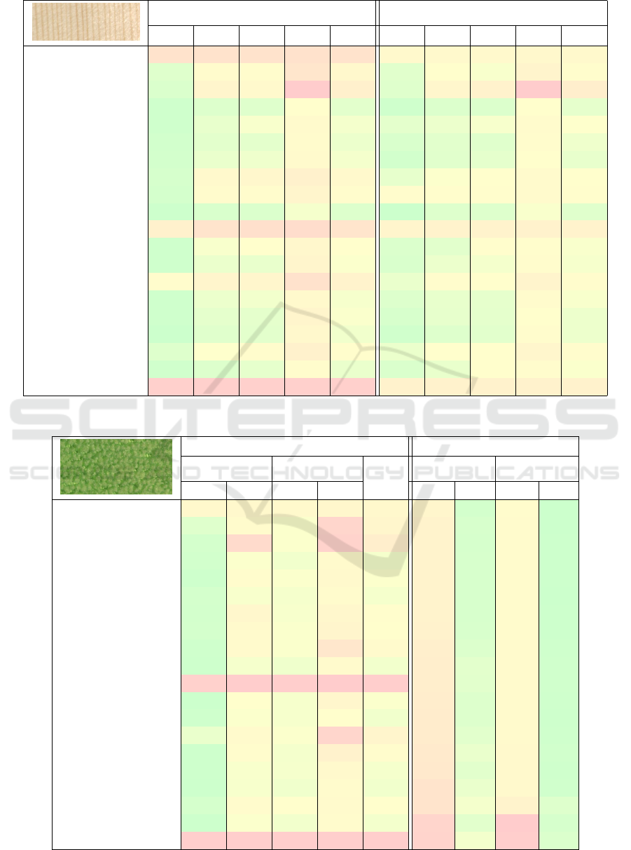
Table 2: BRDF error

ε (median from ﬁve) for spruce.

15–30–20 3–6–4

va-ia vs-ia va-is vs-is ⊘ va-ia vs-ia va-is vs-is ⊘

LINEAR 23.92 23.99 24.01 24.25 24.04 23.94 23.98 24.13 24.24 24.07

SIGMOID 3.13 8.01 7.70 21.89 10.18 8.47 13.11 11.49 33.09 16.54

EXPONENTIAL 2.72 12.08 9.45 38.73 15.74 8.09 28.58 36.02 105.8 44.62

TANH 1.74 2.98 3.16 6.18 3.52 5.95 7.66 7.74 14.73 9.02

RELU 1.76 3.89 5.21 8.93 4.95 8.89 9.86 11.42 19.18 12.34

ELU 1.96 3.44 3.59 7.98 4.24 7.31 8.51 8.34 16.78 10.23

SELU 2.11 4.07 4.45 9.05 4.92 6.27 8.45 8.94 13.35 9.25

SOFTPLUS 2.32 9.84 10.78 14.91 9.46 9.13 12.03 13.32 21.66 14.03

TANHSHRINK 2.14 8.25 7.69 12.39 7.62 12.75 14.83 15.23 21.64 16.11

SOFTSIGN 1.59 2.58 2.77 5.01 2.99 5.54 8.01 7.99 11.72 8.31

HARDSHRINK 14.90 22.83 25.42 27.93 22.77 30.87 35.20 33.66 36.70 34.11

LISHT 1.71 5.24 6.10 11.24 6.07 7.59 8.61 15.03 15.31 11.63

SWISH 1.71 4.13 3.94 12.42 5.55 7.37 9.92 10.95 16.96 11.30

HARDSIGMOID 5.85 12.12 11.76 24.15 13.47 9.59 12.61 13.06 33.35 17.15

SNAKE 1.74 4.18 4.73 9.68 5.08 7.86 9.36 9.08 19.84 11.53

MISH 1.70 3.64 3.63 12.56 5.38 7.02 9.24 8.96 14.59 9.95

GELU 1.50 3.20 3.43 10.49 4.65 6.03 7.96 8.60 17.38 9.99

SOFTMAX 3.02 5.73 5.83 14.58 7.29 9.75 13.89 13.85 29.33 16.70

RRELU 1.79 2.98 3.67 7.73 4.04 7.50 9.39 13.16 17.24 11.82

SOFTSHRINK 35.96 35.96 36.05 36.05 36.01 35.96 35.97 36.03 36.05 36.00

Table 3: BRDF error

ε and learning time for green cloth.

error (median from ﬁve) time [s] (avg. from ﬁve)

15–30–20 3–6–4

⊘

15–30–20 3–6–4

va-ia vs-is va-ia vs-is va-ia vs-is va-ia vs-is

LINEAR 6.44 6.53 6.43 6.91 6.58 784 296 616 258

SIGMOID 2.86 5.84 4.48 15.84 7.25 857 318 646 256

EXPONENTIAL 2.21 14.42 4.45 16.71 9.45 858 317 647 259

TANH 2.14 4.49 3.90 6.07 4.15 859 319 647 258

RELU 1.87 5.38 4.47 6.42 4.53 860 319 649 260

ELU 2.25 4.32 4.12 5.86 4.14 869 320 641 256

SELU 2.19 6.83 4.24 6.95 5.05 872 320 643 258

SOFTPLUS 2.23 5.97 4.43 7.36 5.00 904 328 656 259

TANHSHRINK 1.97 5.90 4.43 11.21 5.88 974 352 670 270

SOFTSIGN 1.88 4.11 3.77 5.97 3.93 993 389 673 276

HARDSHRINK 17.31 18.40 18.15 18.66 18.13 998 386 673 277

LISHT 1.78 4.96 4.16 7.04 4.48 1015 353 680 270

SWISH 1.94 4.45 4.18 5.01 3.89 1045 352 685 265

HARDSIGMOID 3.48 5.94 4.47 16.07 7.49 1063 386 665 274

SNAKE 1.87 4.69 4.04 8.12 4.68 1110 427 695 282

MISH 1.88 4.31 4.10 6.25 4.14 1134 386 700 273

GELU 1.82 4.24 3.84 5.70 3.90 1248 426 716 277

SOFTMAX 2.31 5.81 4.93 6.12 4.79 1263 485 869 363

RRELU 1.84 4.47 3.96 5.85 4.03 1661 385 1892 313

SOFTSHRINK 18.17 18.30 18.17 18.30 18.23 1688 479 1834 345

GRAPP 2023 - 18th International Conference on Computer Graphics Theory and Applications

166

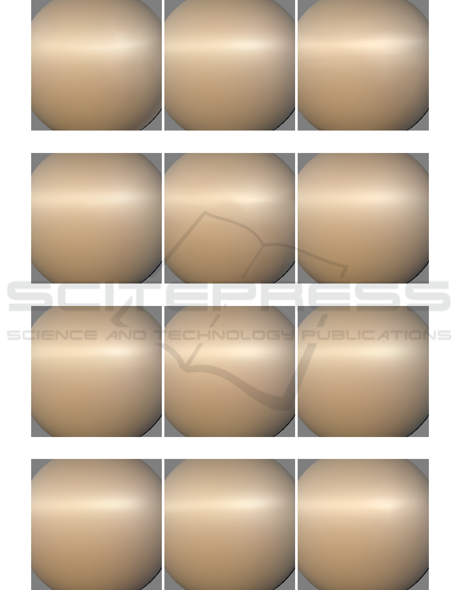
measured + interpolated Tanh (1.70) ReLu (2.02)

ELU (1.79) SELU (1.83) SoftPlus (1.46)

SoftSign (1.97) LiSHT (1.65) Swish (1.84)

Mish (1.66) GELU (1.45) rReLu (2.13)

Figure 5: Spruce rendered modeling results (model 15–30–20 with va-ia) with rendering errors.

Optimal Activation Function for Anisotropic BRDF Modeling

167

artifacts are more visible on lustrous materials (Fig. 5)

than on the matted materials.

Tab. 3 shows the average model learning time of

speciﬁc activation functions in seconds. Apart from

the fastest linear activation function, the fastes nonlin-

ear functions are Sigmoid, Exponential, Tanh, ReLu,

ELU, and SELU. SoftSign is only 12% slower than

the fastest Sigmoid function. SoftShrink evaluation

has the most time expensive evaluation (209%).

Tabs. 2,3 show that the best modeling interpola-

tion is achieved if we teach the model from all view-

ing and illumination angles (Fig. 5). The modeling er-

ror results of the smaller NN-BRDF model are more

stable during training data subsampling. Tab. 2 shows

a modeling improvement if we teach the model from

all illumination angles but only sixth viewing angles

(vs-ia) in comparison with all viewing angles and only

sixth illumination angles (va-is) for both models and

the spruce wood. The maximal △

ε error is 2.6

(10%). If the models are learned from only sixth illu-

mination and viewing angles (vs-is) (3% of measure-

ments, the SoftSign activation function is the most ro-

bust with an average error increase △

ε = 3.4, Tanh is

only slightly worse.

Fig. 1 illustrates the estimated NN-BRDF results

and their enhanced pixelwise differences from the

measured spruce and green cloth anisotropic BRDFs.

The median precision over all activation functions for

both compared BRDF’s (Tabs. 2,3) is in the range of

the average spectral modeling error 2.0 − 12.4 and

(4.3%− 19.5%) for larger and smaller model, respec-

tively. The performance of our BRDF model was also

compared with six anisotropic analytical BRDF mod-

els. Their spectral mean BRDF interpolation error for

the spruce material is in the range of 14 for the best

Phong model (Phong, 1975) to 108 for the worst Ed-

wards model (Edwards et al., 2006).

For additional and more detailed results see

https://mosaic.utia.cas.cz/23GRAPP/.

5 CONCLUSION

The presented anisotropic neural NN-BRDF models

allow us to accurately model anisotropic and isotropic

BRDF for various materials with less than 2.8% aver-

age error increase from only 3% of the original mea-

surements. This almost 97% measurement reduction

saves measurement costs and time signiﬁcantly. The

models learn from more informative BTF data than

usually restricted BRDF measurements.

The best activation function for all tested mate-

rials is SoftSign, followed by Tanh, GELU, ELU,

and SELU from all tested twenty activation functions.

Visual quality comparison of our NN-BRDF models

conﬁrms the same ranking. The non-smooth func-

tional parts of activation functions produce apparent

visual defects. These signiﬁcant artifacts are visible

if mapped on curved object surfaces; thus, they can-

not be used for realistic NN-BRDF modeling.

The extensive UTIA BTF / BRDF database ver-

iﬁed all modeling results with stable results on var-

ied wood species and several other materials. The

model results are also illustrated on textile and spruce

anisotropic materials. The presented model can re-

construct the fully measured angular BRDF hemi-

sphere from sparse measurements and predict an un-

measured, high-resolution BRDF hemisphere from a

low-resolution measurement net. We have also fa-

vorably compared our numerical as well as visual

results with several analytical previously published

BRDF models and planned to publish these results

elsewhere. The presented models can be used directly

as a fast replacement of a BRDF, comparable to fast

analytic BRDF models, in a rendering engine. They

simultaneously offer a high compression rate and in-

terpolation of unmeasured angles.

ACKNOWLEDGMENTS

The Czech Science Foundation project GA

CR 19-

12340S supported this research.

REFERENCES

Ashikhmin, M. and Shirley, P. (2000). An anisotropic phong

brdf model. Journal of graphics tools, 5(2):25–32.

Bell, S., Upchurch, P., Snavely, N., and Bala, K. (2015).

Material recognition in the wild with the materials in

context database. In Proceedings of the IEEE con-

ference on computer vision and pattern recognition,

pages 3479–3487.

Blinn, J. F. (1977). Models of light reﬂection for computer

synthesized pictures. In Proceedings of the 4th an-

nual conference on Computer graphics and interac-

tive techniques, pages 192–198. ACM Press.

Chen, Z., Nobuhara, S., and Nishino, K. (2021). Invertible

neural brdf for object inverse rendering. IEEE Trans-

actions on Pattern Analysis and Machine Intelligence,

pages 1–1.

Cook, R. L. and Torrance, K. E. (1982). A reﬂectance model

for computer graphics. ACM Transactions on Graph-

ics (TOG), 1(1):7–24.

Dahlan, H. A. and Hancock, E. R. (2016). Absorptive

scattering model for rough laminar surfaces. In 2016

23rd International Conference on Pattern Recognition

(ICPR), pages 1905–1910. IEEE.

GRAPP 2023 - 18th International Conference on Computer Graphics Theory and Applications

168

Edwards, D., Boulos, S., Johnson, J., Shirley, P.,

Ashikhmin, M., Stark, M., and Wyman, C. (2006).

The halfway vector disk for brdf modeling. ACM

Transactions on Graphics (TOG), 25(1):1–18.

Fan, J., Wang, B., Ha

san, M., Yang, J., and Yan, L.-Q.

(2021). Neural brdfs: Representation and operations.

arXiv preprint arXiv:2111.03797.

Gibert, X., Patel, V. M., and Chellappa, R. (2015). Mate-

rial classiﬁcation and semantic segmentation of rail-

way track images with deep convolutional neural net-

works. In 2015 IEEE International Conference on Im-

age Processing (ICIP), pages 621–625. IEEE.

Haindl, M. and Filip, J. (2013). Visual Texture. Advances in

Computer Vision and Pattern Recognition. Springer-

Verlag London, London.

Haindl, M., Filip, J., and V

avra, R. (2012). Digital material

appearance: the curse of tera-bytes. ERCIM News,

(90):49–50.

Haindl, M., Mike

s, S., and Kudo, M. (2015). Unsuper-

vised surface reﬂectance ﬁeld multi-segmenter. In Az-

zopardi, G. and Petkov, N., editors, Computer Anal-

ysis of Images and Patterns, volume 9256 of Lecture

Notes in Computer Science, pages 261 – 273. Springer

International Publishing.

Lafortune, E., Foo, S., Torrance, K., and Greenberg, D.

(1997). Non-linear approximation of reﬂectance func-

tions. In ACM SIGGRAPH 97, pages 117–126. ACM

Press.

Minnaert, M. (1941). The reciprocity principle in lunar pho-

tometry. The Astrophysical Journal, 93:403–410.

Ngan, A., Durand, F., and Matusik, W. (2005). Experimen-

tal analysis of brdf models. In Proceedings of the Six-

teenth Eurographics Conference on Rendering Tech-

niques, EGSR ’05, page 117–126, Goslar, DEU. Eu-

rographics Association.

Nielsen, J. B., Jensen, H. W., and Ramamoorthi, R. (2015).

On optimal, minimal brdf sampling for reﬂectance ac-

quisition. ACM Trans. Graph., 34(6):186:1–186:11.

Oren, M. and Nayar, S. K. (1994). Generalization of lam-

bert’s reﬂectance model. In Proceedings of the 21st

annual conference on Computer graphics and inter-

active techniques, pages 239–246.

Phong, B. T. (1975). Illumination for computer generated

pictures. Communications of the ACM, 18(6):311–

317.

Ragheb, H. and Hancock, E. R. (2008). A light scatter-

ing model for layered dielectrics with rough surface

boundaries. International Journal of Computer Vi-

sion, 79(2):179–207.

Schlick, C. (1993). A customizable reﬂectance model for

everyday rendering. In Fourth Eurographics Work-

shop on Rendering, pages 73–83. Paris, France.

Shamir, G. I., Lin, D., and Coviello, L. (2020). Smooth ac-

tivations and reproducibility in deep networks. arXiv

preprint arXiv:2010.09931.

Strauss, P. S. (1990). A realistic lighting model for com-

puter animators. IEEE Computer Graphics and Ap-

plications, 10(6):56–64.

Sztrajman, A., Rainer, G., Ritschel, T., and Weyrich, T.

(2021). Neural brdf representation and importance

sampling. In Computer Graphics Forum, volume 40,

pages 332–346. Wiley Online Library.

Torrance, K. E. and Sparrow, E. M. (1966). Off-specular

peaks in the directional distribution of reﬂected ther-

mal radiation. Journal of Heat Transfer, 6(7):223–

230.

Varma, M. and Zisserman, A. (2009). A statistical ap-

proach to material classiﬁcation using image patch ex-

emplars. IEEE Transactions on Pattern Analysis and

Machine Intelligence, 31(11):2032–2047.

von Helmholtz, H. (1867). Handbuch der physiologischen

Optik, volume 9. Leipzig: Voss.

Ward, G. (1992). Measuring and modeling anisotropic re-

ﬂection. Computer Graphics, 26(2):265–272.

Xu, Z., Nielsen, J. B., Yu, J., Jensen, H. W., and Ramamoor-

thi, R. (2016). Minimal brdf sampling for two-shot

near-ﬁeld reﬂectance acquisition. ACM Trans. Graph.,

35(6).

Zheng, C., Zheng, R., Wang, R., Zhao, S., and Bao, H.

(2021). A compact representation of measured brdfs

using neural processes. ACM Trans. Graph., 41(2).

Optimal Activation Function for Anisotropic BRDF Modeling

169