Detection of Microscopic Fungi and Yeast in Clinical Samples Using

Fluorescence Microscopy and Deep Learning

Jakub Paplh

, Vojt

ech Franc

and Daniela L

rov

Department of Cybernetics, Czech Technical University in Prague, Prague, Czech Republic

Second Faculty of Medicine, Charles University, Prague, Czech Republic

Keywords:

Filamentous Fungi, Yeast, Automated Detection, Fluorescence Staining, Poisson Image Editing.

Abstract:

Early detection of yeast and ﬁlamentous fungi in clinical samples is critical in treating patients predisposed to

severe infections caused by these organisms. The patients undergo regular screening, and the gathered samples

are manually examined by trained personnel. This work uses deep neural networks to detect ﬁlamentous fungi

and yeast in the clinical samples to simplify the work of the human operator by ﬁltering out samples that are

clearly negative and presenting the operator with only samples suspected of containing the contaminant. We

propose data augmentation with Poisson inpainting and compare the model performance against expert and

beginner-level humans. The method achieves human-level performance, theoretically reducing the amount of

manual labor by 87%, given a true positive rate of 99% and incidence rate of 10%.

1 INTRODUCTION

Early detection of yeast and ﬁlamentous fungi in clin-

ical samples is critical in treating patients predisposed

to severe infections caused by these organisms. Fluo-

rescence microscopy is a suitable method for this de-

tection, where after application to a slide, the mate-

rial is stained with a ﬂuorescent dye (e.g., Calcoﬂuor

White), which binds to chitin contained in the fun-

gal cell wall. This staining process is non-speciﬁc,

as other structures that may occur accidentally in the

sample (e.g., dust, pollen, arthropods) can also bind

the dye. Clinical samples commonly consist of res-

piratory secretions or non-invasive tissue biopsy sam-

ples; the aforementioned foreign bodies are therefore

routinely present.

Severe infections caused by ﬁlamentous fungi are

sporadic but severe. Patients with a risk factor, there-

fore, undergo regular screening. It follows that a con-

siderable number of slides must be carefully exam-

ined, most of which do not contain yeast or ﬁlamen-

tous fungi.

This work was done in collaboration with Motol

University Hospital in Prague, whose staff amassed

a unique dataset of ﬂuorescence microscopy images

over a period of several years. The goal of the col-

laboration is to develop an automated system, which

ﬁlters out samples that are easily distinguishable as

negative and presents the remaining potentially posi-

tive samples to an expert for veriﬁcation.

Currently, fungi and yeast cells are detected manu-

ally by trained personnel. Laboratory staff then spend

a signiﬁcant amount of time examining negative sam-

ples, which leads to job dissatisfaction, and the devel-

opment of musculoskeletal disorders caused by repet-

itive stress injuries. Deployment of the system would

therefore lead to reduction of the amount of manual

labor and an increase in the quality of work.

This paper represents a feasibility study for au-

tomation and uses mostly standard deep learning

methods. In actual deployment, the detector will be

applied to a sequence of images obtained from an au-

tomated microscope rather than a single image.

Our main contributions are the following: (i) a

detector based on convolutional neural networks

(CNNs) is trained on a unique dataset,, (ii) a data aug-

mentation technique speciﬁc to the detection task is

proposed,, or (iii) performance of the model is eval-

uated and compared against expert and novice level

humans.

2 RELATED WORKS

Recently, automated slide scanners were used for

slide imaging of clinical samples and CNNs for eval-

uation of the data. This allows for fully automatic de-

Paplhám, J., Franc, V. and Lži

rová, D.

Detection of Microscopic Fungi and Yeast in Clinical Samples Using Fluorescence Microscopy and Deep Learning.

DOI: 10.5220/0011616100003417

In Proceedings of the 18th International Joint Conference on Computer Vision, Imaging and Computer Graphics Theory and Applications (VISIGRAPP 2023) - Volume 4: VISAPP, pages

777-784

ISBN: 978-989-758-634-7; ISSN: 2184-4321

 2023 by SCITEPRESS – Science and Technology Publications, Lda. Under CC license (CC BY-NC-ND 4.0)

777

tection and classiﬁcation of microscopic organisms.

The approach has been successfully used for the

detection of bacteria in Gram stains of blood culture,

(Smith et al., 2018), and detection of intestinal pro-

tozoa in trichrome stained stool samples, (Mathison

et al., 2020). Gram staining dyes were also applied

to samples containing yeast and yeast-like fungi, al-

lowing their successful classiﬁcation, (Zieli

nski et al.,

2020). Perhaps most similar to the goals of this work,

(Gao et al., 2021) fully automate the process of scan-

ning and classifying ﬂuorescent dye-stained skin sam-

ples containing fungi.

All of the listed methods utilize the industry stan-

dard technique of ﬁne-tuning a pre-trained CNN.

They employ an automated scanner to obtain a large

number of images from each sample, classify the im-

ages separately, then aggregate the result over the im-

ages to classify the sample. An identical approach can

be observed in the entire ﬁeld of automatic evaluation

of digital microscopy.

The methods achieve human-level performance,

motivating future large-scale deployment. Some nov-

elty can be observed in the use of non-standard clas-

siﬁer heads, e.g., (Zieli

nski et al., 2020) replace the

linear classiﬁcation head with bag-of-words encoding

followed by a support vector machine (SVM) classi-

ﬁer. To our knowledge, no notable domain-speciﬁc

modiﬁcations of the standard techniques were used in

these works.

Our work focuses on a different domain, namely

ﬂuorescent microscopy of human secretions. Further,

we are presented with only a single image per sample

and demonstrate that the method achieves sufﬁcient

performance for deployment even in this setting.

3 METHODS

3.1 Dataset

The dataset contains high-resolution images of sam-

ples collected by staff of Motol University Hospital in

Prague from January 2018 to April 2021. The images

are a priori assumed to be negative and are considered

positive only when structures speciﬁc to microscopic

yeast or fungi are detected, even if low-resolution and

present only in a small portion of the image. An ex-

ample of such a case, where a single yeast cell is

present and covers only a very small portion of the

image, is shown in Figure 3.

The dataset contains a total of 1244 high-

resolution images. The pixel dimensions of the im-

ages are not identical, see Table 1. However, the

aspect ratio

Width

Height

≈ 1.33 is constant throughout the

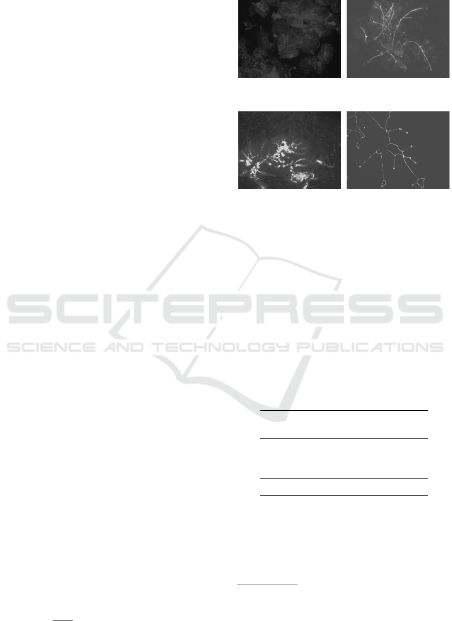
Figure 1: Showcase of randomly selected positive samples

from the dataset.

Figure 2: Showcase of randomly selected negative samples

from the dataset.

dataset, and each image captures the same ﬁeld of

view. The images can therefore be resized to a

uniform shape, which allows for mini-batching of

the data, improving the training efﬁciency. Annota-

tions are given in the form of the binary label (pos-

itive/negative) for each image. In other words, the

annotation provides no information on the location or

size of the specimen within the image.

The main challenges associated with the dataset

are twofold: (i) the amount of available data is rela-

tively low, and (ii) positive and negative images have

a high degree of similarity. Examples of positive and

negative samples are shown in Figure 1 and Figure 2,

respectively.

Table 1: Dimensions of images in the dataset.

Width × Height

Annotation

Positive Negative

4140 ×3096 374 546

2040 ×1536 77 3

1360 ×1024 231 13

Total 682 562

Sample Preparation. Clinical Material

was

smeared on a sterile slide and dried. The dried slides

were dyed with Calcoﬂuor White mixed 1 : 1 with

20% potassium hydroxide solution and immediately

covered with cover slides and examined. Fluores-

cence microscopy was performed manually with the

Speciﬁcally (i) sputum, (ii) endotracheal or bronchial

aspirate, (iii) bronchoalveolar ﬂuid or tissue, (iv) pleu-

ral ﬂuid, (v) pericardial ﬂuid, (vi) cerebrospinal ﬂuid, or

(vii) liquid or solid contents of pathological cavities.

VISAPP 2023 - 18th International Conference on Computer Vision Theory and Applications

778

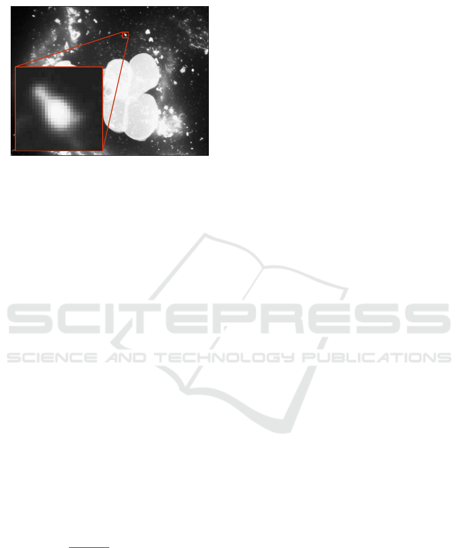
Figure 3: Except for a single budding yeast cell, there is no

contaminant in the image. The yeast cell takes up only a

small portion of the image, but it is entirely responsible for

the ﬁnal classiﬁcation as a positive sample.

use of Olympus BX 53 ﬂuorescence microscope, Up-

lanFLN 20x objective lens, FN 26,5. The entire slide

was examined, and a representative section of the

slide was selected. The image of the selected section

was captured using an Olympus DP72 microscope

digital camera.

3.2 Model

Formal Deﬁnition. Let us denote the common

pixel domain as D ⊂ Z

, and the monochromatic do-

main as M ⊂ {x | x ∈ R}, where lower and upper

bounds of the values and machine precision are ig-

nored for simplicity. The set of all possible grayscale

images is then I = M

The model is a binary image classiﬁer, i.e., the

mapping h : X → Y , where X ⊂ I , Y = {+1, −1}.

Often the classiﬁer h is further decomposed as

h = f ◦d, where f : X → R, and d : R → {+1,−1},

with the decoding mapping d deﬁned as

d(x,θ) =

(

+1 for x ≥ θ,

−1 for x < θ,

for some ﬁxed threshold θ ∈R. We further deﬁne an

ensemble of binary classiﬁers, as a binary classiﬁer

where the score function f is deﬁned as

f (x) =

∑

i=1

(x)

, f

: X → R.

(1)

Implementation. We choose ResNet-50 with a sin-

gle linear output layer as our baseline binary classiﬁer

f and use the shallower variant, ResNet-18, to search

for an optimal training setup, e.g., data augmentations

and image preprocessing. We further train and com-

pare performance of (i) ResNet-50x1-V2, (He et al.,

2016), (ii) EfﬁcientNet models, (Tan and Le, 2019),

from B0 to B4, (iii) EfﬁcientNet-V2-S model, (Tan

and Le, 2021), and (iv) Vision Transformer ViT-B us-

ing 32 ×32 embeddings (Dosovitskiy et al., 2021).

All models we use are pretrained on ImageNet.

3.3 Saved Time Metric

Assuming that manual examination of each sample

takes constant time, the amount of human time saved

by the model is directly proportional to the number

of samples which need not be examined by human

personnel. If a sample is to be classiﬁed as positive,

manual conﬁrmation is required. Therefore, the saved

time is proportional to the number of samples classi-

ﬁed as negative by the model.

The maximal value of such a metric can be

achieved by classifying all samples as negative. This

is clearly undesirable. Therefore, we deﬁne the saved

time metric as the portion of samples classiﬁed as

negative while guaranteeing that the true positive rate

is higher than a speciﬁed level. The metric represents

an alternative to the standard ROC curve. It directly

measures the clinical utility of the model and can eas-

ily be explained to medical staff.

Formal Deﬁnition. We evaluate the prediction

rule h: X → {+1, −1} in terms of two metrics.

First, the true positive rate (a.k.a. sensitiv-

ity) TPR(h) = E

x∼p(x|y=+1)

[[h(x) = +1]], which is

the probability that a positive sample is correctly

classiﬁed as positive. Secondly, the saved time

ST(h) = E

x∼p(x)

[[h(x) = −1]], equal to the probabil-

ity that any input sample is classiﬁed as negative. It is

useful to rewrite the saved time as

ST(h) =



1 −p(y = +1)





1 −FPR(h)



+ p(y = +1) ·



1 −TPR(h)



(2)

where p(y = +1) is the prior probability of the posi-

tive class, and FPR(h) = E

x∼p(x|y=−1)

[[h(x) = +1]] is

the false positive rate, i.e., the probability that a neg-

ative sample is incorrectly classiﬁed as positive. The

equation (2) shows that the two metrics, TPR(h) and

ST(h), are antagonistic, i.e., increasing one leads to a

decrease of the other and vice versa.

Evaluating the Metric. As deﬁned in Section 3.2,

the model is a binary image classiﬁer of the form

h(x;θ) =

(

+1 for f (x) ≥ θ,

−1 for f (x) < θ,

(3)

where f : X → R is a score function trained from ex-

amples and θ ∈ R is a decision threshold used to tune

Detection of Microscopic Fungi and Yeast in Clinical Samples Using Fluorescence Microscopy and Deep Learning

779

the operating point of the model. With a slight abuse

of notation, we use TPR(θ) and ST(θ) as a shortcut

for TPR(h(·;θ)) and ST(h(·;θ)), respectively.

The number of positive and negative samples in

the available test set is approximately the same, which

does not match the real distribution at the deploy-

ment time. According to Motol University Hospi-

tal’s staff, approximately 9 out of 10 samples that ar-

rive at the laboratory for examination are negative.

Therefore, when evaluating the detector we assume

that the incidence rate is p(y = +1) = 0.1. How-

ever, the methodology as a whole is general and,

if necessary, can be applied to any incidence rate.

When evaluating the metric, we resolve the men-

tioned distribution mismatch as follows. Given a test

set {(x

) ∈ X ×{+1,−1}| i = 1, ..., n}, we com-

pute the empirical estimates of TPR(θ) and FPR(θ),

TPR(θ) =

∑

i=1

[[h(x

;θ) = +1 ∧y

= +1]], (4)

FPR(θ) =

−

∑

i=1

[[h(x

;θ) = +1 ∧y

= −1]], (5)

where n

∑

i=1

[[y

= +1]] and n

−

∑

i=1

[[y

= −1]].

Then, we ﬁx the positive class prior to the expert

estimate of the incidence rate, p(y = +1) = 0.1,

and compute the empirical estimate of the saved

time

ST(θ) by substituting

TPR(θ) and

FPR(θ)

into equation (2). We evaluate the predictor h

by a curve

n

TPR(θ) ,

ST(θ)



| θ ∈ (−∞,∞)

which summarizes the entire space of achievable

true positive rates and saved times. As a ref-

erence, we also plot the best achievable saved

time curve as a function of TPR, i.e., we plot

the curve

{

(TPR,ST

∗

(TPR)) | TPR ∈(0,1)

}

where

∗

(TPR) = p(y = +1) ·[1 −TPR] + [1 − p(y = +1)],

which is obtained from equation (2) when assuming

an ideal predictor with zero FPR(h).

In case we need to evaluate the predictor by a sin-

gle scalar, e.g., when ranking different models, we

report the saved time at desired true positive rate τ,

which is deﬁned as

= max

θ∈(−∞,∞)

ST(θ) subject

TPR(θ) ≥ τ .

3.4 Domain-Speciﬁc Data

Augmentation

To enlarge the number of samples used for train-

ing, we utilize standard image data augmentations,

namely (i) horizontal ﬂip, (ii) vertical ﬂip, (iii) rota-

tion, and (iv) crop and resize. We also implement and

evaluate the effects of a custom augmentation method

described in the following text.

Motivation & Overview. While obtaining negative

samples is simple, getting positive samples is com-

paratively complex and expensive. We propose an

augmentation method speciﬁc to the detection task,

where any negative image becomes positive if the

contaminant (e.g., yeast or fungi) is introduced. The

technique takes advantage of a large number of nega-

tive images and uses them to generate synthetic pos-

itive images by inpainting the positive contaminant

into a negative background. The contaminant can fur-

ther be rotated and shifted to create practically an un-

limited number of positive samples.

To generate additional positive samples, we locate

the fungi or yeast within the image either by (i) gradi-

ent-based localization, Grad-CAM (Selvaraju et al.,

2017), which is a broadly applicable method with

minimal prerequisites, or (ii) by exploiting the ﬂuo-

rescent staining process. We then augment the image

by inpainting the located yeast and fungi into a nega-

tive background using Poisson image editing, (P

erez

et al., 2003).

We also generate synthetic negative samples, to

keep the augmentation symmetrical with respect to

classes; preventing the model from associating poten-

tial inpainting artifacts with the positive class. In neg-

ative samples, we inpaint structures that are visually

similar to the yeast and fungi, localized using Grad-

CAM, (Selvaraju et al., 2017).

Overview of Poisson Inpainting. Consider the task

of inpainting a portion of a source image s into a back-

ground b to form a resulting image r . The naive ap-

proach is to directly copy the pixel values from the

source s to the background b. This, however, cre-

ates visible edges between the inpainted region and

the background. Instead of copying values of the pix-

els, Poisson image editing, (P

erez et al., 2003), copies

the gradient. A comparison with the naive procedure

is shown in Figure 6.

To inpaint a region of the source into the back-

ground using Poisson inpainting, (i) pixels on the bor-

der of the source region are set to match the neighbor-

ing pixels in the background, and (ii) the remaining

pixel values of the inpainted source region are found

by solving the Poisson equation with the condition of

preserving the gradient of the source image. I.e., the

color of the inpainted region is modiﬁed to match the

color of the background, but the relative color differ-

ence between pixels is preserved.

Formal Deﬁnition of Poisson Inpainting. Here,

we brieﬂy review our usage of the method famously

introduced by (P

erez et al., 2003). Let us denote a

background image, a source image, and a resulting

VISAPP 2023 - 18th International Conference on Computer Vision Theory and Applications

780

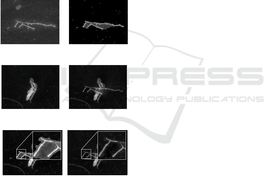
image as b,s,r ∈ I , respectively. By Ω ⊂ D, let us de-

note a region within the source image s which is to be

inpainted into the background b to form the resulting

image r. Let us further denote by p ∈ D a pixel po-

sition and by s

, b

, r

values of the pixel within the

source, background, and result images, respectively.

To seamlessly inpaint the region Ω of the source

image into the background image, we solve the opti-

mization problem

min

∑

⟨p,q⟩∩Ω̸=

−r

−s

+ s

)

, (6)

subject to

= b

, ∀p ∈ δΩ, (7)

where ⟨p,q⟩ is a pixel neighbor pair.

→

Figure 4: Thresholding a ﬂuorescent stained positive sam-

ple to obtain the Ω regions for Poisson inpainting.

→

Figure 5: Synthetic sample created by inpainting region

containing the positive class into a negative background.

Figure 6: Comparison of the inpainting methods. The in-

painted region has a distinct background color when the

value of pixels is copied directly. The Poisson image editing

ensures that the cutout seamlessly blends into the negative

image, creating a more realistic result.

Generating Synthetic Positive Samples. The aug-

mentation procedure requires (i) a positive source im-

age s, (ii) a localization mask deﬁning the region Ω,

and (iii) a negative background image b. To local-

ize the fungi and yeast, we exploit the fact that due

to the ﬂuorescent staining process, the pixel values of

the yeast and fungi are always greater than those of

the background. Therefore, we can obtain a rough lo-

calization mask by thresholding the pixel values, e.g.,

by employing Yen’s non-parametric thresholding al-

gorithm, (Yen et al., 1995). It must be noted that the

ﬂuorescent dye is non-speciﬁc, however, and other

structures, such as dust, pollen, or arthropods, may

also bind the dye. Yeast or fungi is therefore always

inpainted, but some miscellaneous structures are in-

advertently inpainted as well. This, however, does not

harm the creation of new positive examples.

If the localization mask contains multiple con-

nected components, we interpret each connected com-

ponent as a region Ω and inpaint it separately with

random rotation and random position. This modiﬁca-

tion is especially suited for yeast.

The following steps summarize the augmentation:

(i) Localize regions Ω of a positive source image s

which contain yeast or fungi., (ii) Select a negative

background image b at random., or (iii) Inpaint each

region of s discovered in step (i) into the negative im-

age b to form the resulting image. The position and

rotation of the inpainted region within the result are

selected at random.

Generating Synthetic Negative Samples. The

augmentation procedure requires (i) a negative im-

age, serving as both a source s and background b, and

(ii) a localization mask deﬁning the region Ω. We

use the gradient-based Grad-CAM localization, (Sel-

varaju et al., 2017), to discover the Ω regions. Grad-

CAM provides a course heatmap from which we gen-

erate a binary mask by thresholding. It must be men-

tioned that the heatmap speciﬁes the relative magni-

tude of activations of the learned convolutional ﬁlters.

If there are no structures in the image that are similar

to fungi or yeast, the activations across the entire im-

age are of similar magnitude and the resulting mask

covers the entire image. We, therefore, do not aug-

ment the sample in such a case. The following steps

summarize the augmentation: (i) Localize regions Ω

of a negative image that are visually similar to yeast

or fungi., or (ii) Inpaint each region discovered in step

(i) into the image to form the resulting image. The po-

sition and rotation of the inpainted region within the

result are selected at random. This step can be re-

peated multiple times.

4 EXPERIMENTS & RESULTS

Setup. Unless explicitly stated otherwise, we train

and evaluate the models using 30-fold cross-

validation with training, validation, and test sets con-

taining 80%, 10%, and 10% of the total data set, re-

Detection of Microscopic Fungi and Yeast in Clinical Samples Using Fluorescence Microscopy and Deep Learning

781

spectively. We use the SGD optimizer with 0.9 Nes-

terov momentum. The initial learning rate is set to

0.001 and reduced by a factor of 3 upon reaching 33%

and 66% of the 150 total training epochs. We train

using a batch size of 10 images due to hardware limi-

tations. We use images of a uniform size of 952×716

pixels. We show the effects of image size on perfor-

mance of a ResNet-18 model in Figure 7. A larger im-

age size results in better performance; however, an in-

crease over 680 ×512 yields only marginal improve-

ments.

272 × 205

544 × 409

816 × 614

1088 × 819

1360 × 1024

Image Size

0.00

0.25

0.50

0.75

1.00

Saved Time

True Positive Rate

0.98 0.99 0.995

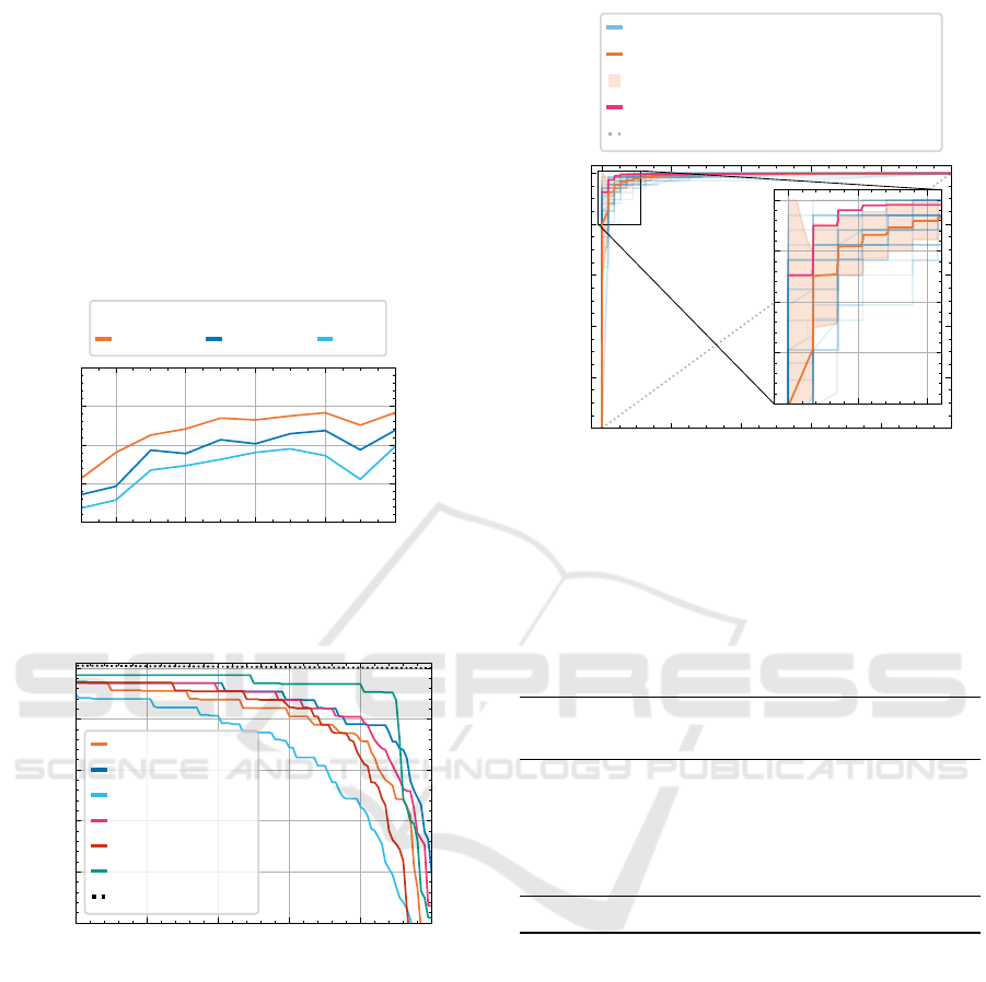
Figure 7: Dependence of saved time metric on image size.

0.95 0.96 0.97 0.98 0.99 1.00

True Positive Rate

0.4

0.5

0.6

0.7

0.8

0.9

Saved Time

ResNet-50

EﬃcientNet-B2

ViT-B-32

EﬃcientNet-V2-S

ResNet-50-V2

Ensemble

Upper Bound

Figure 8: Comparison of different model architectures.

4.1 Model Architecture

We train multiple state-of-the-art models of similar

complexity as ResNet-50. It is well known that en-

sembling techniques result in improved performance

at the cost of increased computational complexity.

We, therefore, also produce an ensemble of the ar-

chitectures by averaging their predictions.

The achieved saved time metric values are dis-

played in Table 2 and the curve of achievable val-

ues is shown in Figure 8. The performance of all

the models is within a 5% margin, except for an

outlier, the Vision Transformer, which performs sig-

0.0 0.2 0.4 0.6 0.8 1.0

True Negative Rate

0.0

0.2

0.4

0.6

0.8

1.0

True Positive Rate

ResNet-50 Instance

Mean (AUC = 0.991)

± 1 Standard Deviation

Ensemble (AUC = 0.997)

Random Classiﬁer

0.00 0.05 0.10

0.80

0.85

0.90

0.95

1.00

Figure 9: ROC curve (receiver operating characteristic) of

ResNet-50 models. The orange curve shows the mean ROC

over all folds, with the light orange area marking the stan-

dard deviation between folds. The pink curve shows the

ROC for an ensemble of different model architectures.

Table 2: Saved time metric comparison for different model

architectures. The ﬁrst value indicates the mean saved time

metric; the second is the standard deviation between folds.

True positive rate

Model 98% 99% 99.5%

RN-50 0.81 (0.12) 0.76 (0.18) 0.64 (0.20)

EN-B2 0.84 (0.05) 0.79 (0.10) 0.76 (0.10)

ViT-B-32 0.74 (0.12) 0.63 (0.18) 0.47 (0.22)

EN-V2-S 0.84 (0.05) 0.81 (0.12) 0.70 (0.12)

RN-50-V2 0.82 (0.08) 0.72 (0.19) 0.56 (0.28)

Ensemble 0.87 (0.03) 0.87 (0.16) 0.84 (0.16)

niﬁcantly worse. The best performance is achieved

by EfﬁcientNet-B2 models, reaching both the highest

value of the saved time metric and the lowest stan-

dard deviation between folds, i.e., the architecture

performs the best consistently. From the EfﬁcientNet

family of models, we only report the best performer,

EfﬁcientNet-B2. By ensembling, the performance

can further be improved, resulting in a theoretical re-

duction of manual labor (saved time) of 87%, given a

true positive rate of 99%. We show the ROC curve in

Figure 9. The ensemble comprises (i) ResNet-50, (ii)

EfﬁcientNet-B2, (iii) ViT-B-32, (iv) EfﬁcientNet-V2-

S, (v) ResNet-50-V2. Score function of the ensem-

ble is computed as the mean of score functions of the

component models.

VISAPP 2023 - 18th International Conference on Computer Vision Theory and Applications

782

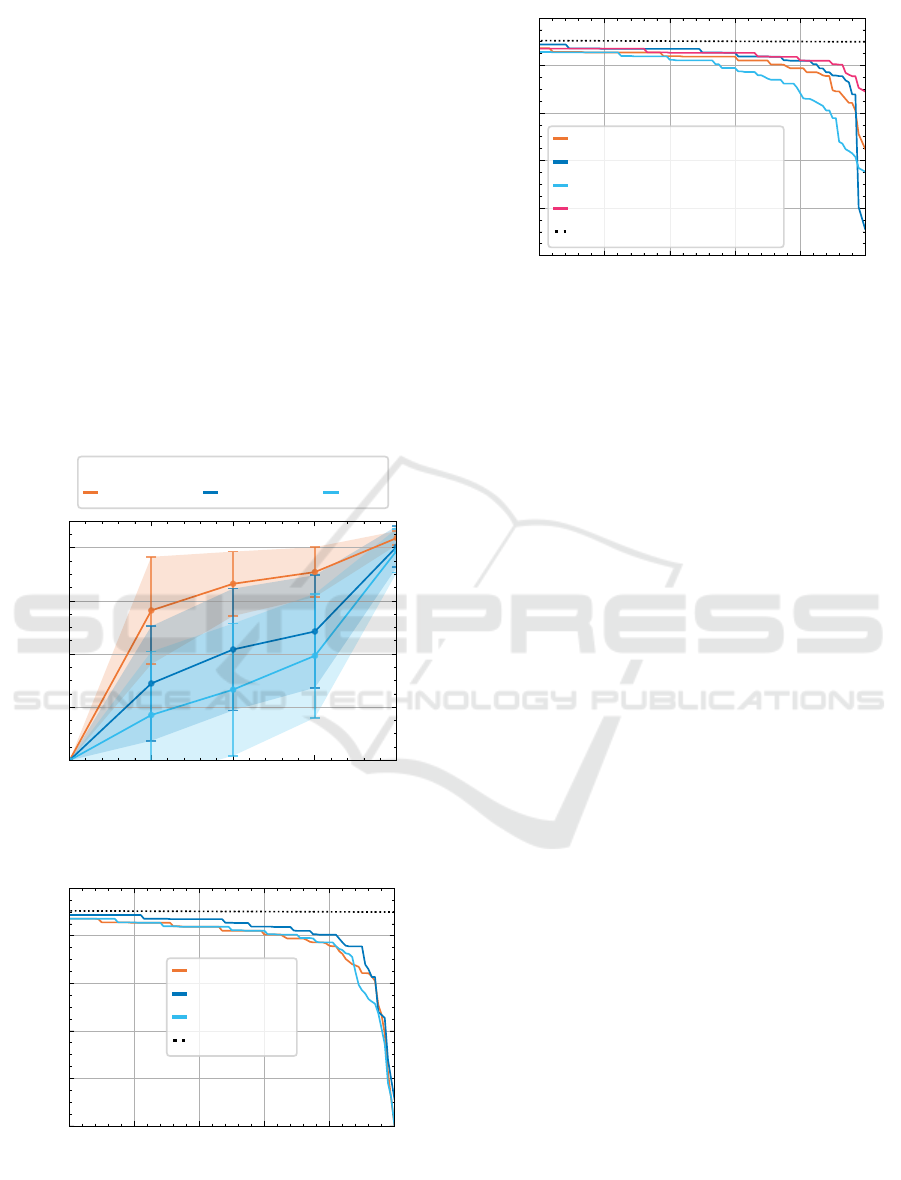
4.2 Poisson Augmentation

We construct a learning curve, shown in Figure 10,

to verify that the model can beneﬁt from a larger

dataset. The performance steeply improves with ad-

ditional data, motivating further data augmentations

beyond the standard techniques.

We train ResNet-50 with additional synthetic pos-

itive samples, which were created either (i) by Pois-

son inpainting, or (ii) by directly copying the pixel

values. The results are shown in Figure 11 and

demonstrate that the Poisson inpainting is crucial, as

the naive technique does not result in any perfor-

mance improvements.

We, therefore, train ResNet-50 with additional

synthetic samples, both positive and negative, created

with Poisson inpainting. Models trained using the

augmentation of both classes consistently outperform

the baseline. The results are shown in Figure 12.

0 25 50 75 100

Dataset Size [%]

0.0

0.2

0.4

0.6

0.8

Saved Time

True Positive Rate

0.98 0.99 0.995

Figure 10: Learning curve for ResNet-50. The transparent

area shows ±1 standard deviation. Result on 11 folds.

0.95 0.96 0.97 0.98 0.99 1.00

True Positive Rate

0.0

0.2

0.4

0.6

0.8

1.0

Saved Time

Baseline

Poisson

Naive Copy

Upper Bound

Figure 11: Training with synthetic positive samples created

with Poisson inpainting results in better performance than

naively copied pixel values. Result on 20 folds.

0.95 0.96 0.97 0.98 0.99 1.00

True Positive Rate

0.0

0.2

0.4

0.6

0.8

1.0

Saved Time

Baseline

Positive Poisson

Negative Poisson

Positive & Negative Poisson

Upper Bound

Figure 12: Training with both, positive and negative, syn-

thetic samples results in signiﬁcant increase in performance.

Result on 15 folds.

4.3 Human-Machine Comparison

To assess the difﬁculty of the task and further eval-

uate the model performance, we select 100 positive

and 100 negative images from the dataset at random

and compare the performance of the model with the

performance of humans on the classiﬁcation.

The images were shown to 4 expert microbiol-

ogists. They were prompted to classify the images

as either positive or negative. A group of 3 begin-

ners was also shown the images after a brief training

session that included a showcase of 20 representative

positive and 20 negative samples. The task was ver-

bally explained, and special attention was given to the

speciﬁc structures of the contaminants.

For each of the images, the automated classiﬁca-

tion was produced by an ensemble model, which con-

tained the given image in its test set.

All expert microbiologists perform similarly,

achieving a true positive rate of 89%, 89%, 90% and

94% with a saved time of 91.1%, 91.1%, 89.2% and

90.6% respectively. The experts achieve values of the

saved time at the theoretical upper bound, i.e., the

experts achieve a false positive rate of FPR ≈ 0. It

should be noted that the presented task is signiﬁcantly

different from the standard operating procedure of the

experts. In the usual setting, the expert is presented

with an entire slide and can freely move between por-

tions of the slide and search for the contaminant. In

this experiment, the view is locked, and the expert is

presented with only a single image.

The beginner-level humans perform signiﬁcantly

worse than the automated model. They either (i) do

not achieve sufﬁcient true positive rate, or (ii) achieve

sufﬁcient true positive rate, but a low value of the

saved time metric. The ensemble of models performs

at the same level or a better level than the expert hu-

mans. The result is shown in Figure 13.

Detection of Microscopic Fungi and Yeast in Clinical Samples Using Fluorescence Microscopy and Deep Learning

783

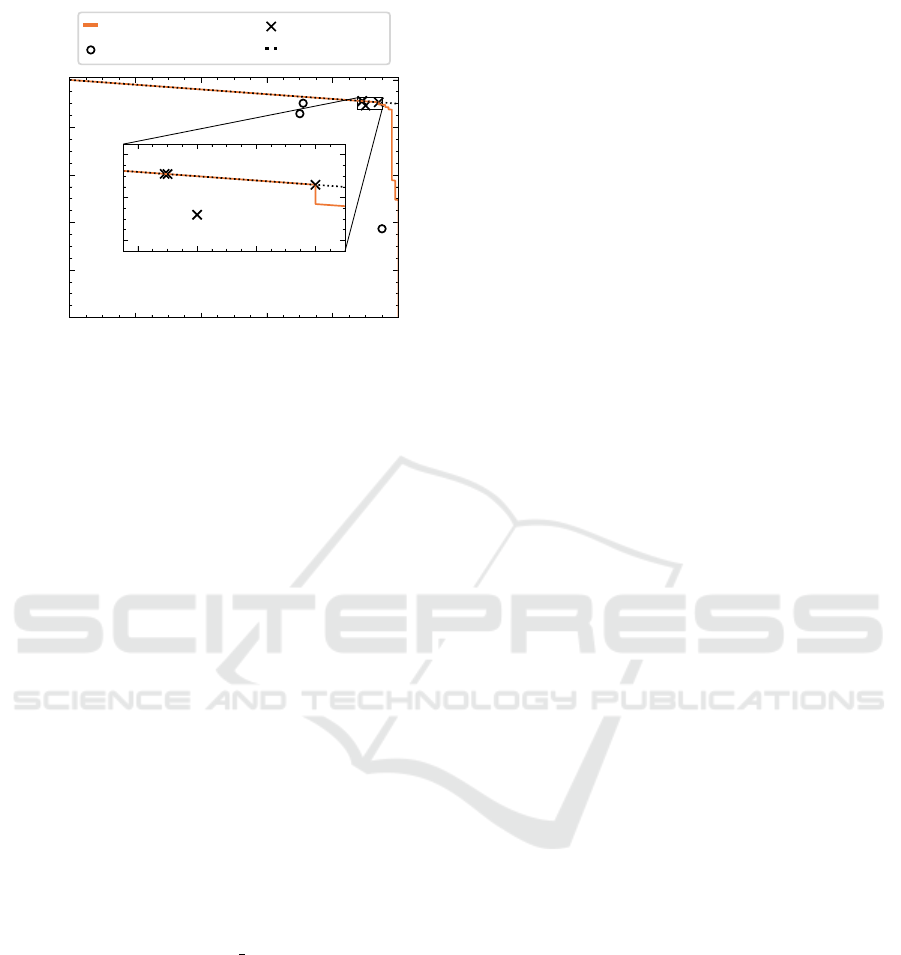
0.0 0.2 0.4 0.6 0.8 1.0

True Positive Rate

0.0

0.2

0.4

0.6

0.8

1.0

Saved Time

Ensemble

Beginner

Expert

Upper Bound

0.88 0.90 0.92 0.94

0.88

0.90

0.92

Figure 13: Human-machine performance comparison. Re-

sults on a randomly selected set of 100 positive and 100 neg-

ative samples. Medical experts perform signiﬁcantly better

than beginner humans, who are outperformed by the auto-

mated model by a signiﬁcant margin.

5 CONCLUSION

The results indicate that the detection of microscopic

yeast and fungi in clinical samples can be tackled by

standard deep-learning methods, employing an en-

semble of convolutional neural networks. The de-

veloped model consistently performs on par or better

than a human expert and, if deployed, should reduce

the amount of manual labor by approximately 87%

when operating at a true positive rate of 99%. The re-

sults are achieved with annotations only on the image

level, i.e., the network was not instructed what part of

the image is responsible for the classiﬁcation.

ACKNOWLEDGEMENTS

The authors acknowledge the support of the OP VVV

project CZ.02.1.01/0.0/0.0/16 019/0000765 Research

Center for Informatics. The paper also acknowledges

project No. VJ02010041 supported by the Ministry

of the Interior of the Czech Republic. Special thanks

belongs to MUDr. Daniela L

rov

a for collecting

the dataset and to MUDr. Kamila Dundrov

a, MUDr.

Vanda Chrenkov

a, Bc. Karla Ka

nkov

a, Vladim

ır

Kryll, RNDr. Pavl

ına Lyskov

a, Ph. D. for ﬁlling out

the human-machine comparison survey.

REFERENCES

Dosovitskiy, A., Beyer, L., Kolesnikov, A., Weissenborn,

D., Zhai, X., Unterthiner, T., Dehghani, M., Min-

derer, M., Heigold, G., Gelly, S., Uszkoreit, J., and

Houlsby, N. (2021). An image is worth 16x16 words:

Transformers for image recognition at scale. ArXiv,

abs/2010.11929.

Gao, W., Li, M., Wu, R., Du, W., Zhang, S., Yin, S., Chen,

Z., and Huang, H. (2021). The design and appli-

cation of an automated microscope developed based

on deep learning for fungal detection in dermatology.

Mycoses, 64(3):245–251.

He, K., Zhang, X., Ren, S., and Sun, J. (2016). Identity

mappings in deep residual networks.

Mathison, B. A., Kohan, J. L., Walker, J. F., Smith,

R. B., Ardon, O., Couturier, M. R., and Pritt, B. S.

(2020). Detection of intestinal protozoa in trichrome-

stained stool specimens by use of a deep convolutional

neural network. Journal of Clinical Microbiology,

58(6):e02053–19.

erez, P., Gangnet, M., and Blake, A. (2003). Poisson im-

age editing. ACM Trans. Graph., 22(3):313–318.

Selvaraju, R. R., Cogswell, M., Das, A., Vedantam, R.,

Parikh, D., and Batra, D. (2017). Grad-cam: Visual

explanations from deep networks via gradient-based

localization. In 2017 IEEE International Conference

on Computer Vision (ICCV), pages 618–626.

Smith, K. P., Kang, A. D., and Kirby, J. E. (2018). Auto-

mated interpretation of blood culture gram stains by

use of a deep convolutional neural network. Journal

of Clinical Microbiology, 56(3):e01521–17.

Tan, M. and Le, Q. (2019). EfﬁcientNet: Rethinking model

scaling for convolutional neural networks. In Chaud-

huri, K. and Salakhutdinov, R., editors, Proceedings of

the 36th International Conference on Machine Learn-

ing, volume 97 of Proceedings of Machine Learning

Research, pages 6105–6114. PMLR.

Tan, M. and Le, Q. V. (2021). Efﬁcientnetv2: Smaller mod-

els and faster training. ArXiv, abs/2104.00298.

Yen, J.-C., Chang, F.-J., and Chang, S. (1995). A new

criterion for automatic multilevel thresholding. IEEE

Transactions on Image Processing, 4(3):370–378.

Zieli

nski, B., Sroka-Oleksiak, A., Rymarczyk, D., Piekar-

czyk, A., and Brzychczy-Włoch, M. (2020). Deep

learning approach to describe and classify fungi mi-

croscopic images. PLOS ONE, 15(6):1–16.

VISAPP 2023 - 18th International Conference on Computer Vision Theory and Applications

784