Condition for Sustained Oscillations in Repressilator Based on a Hybrid

Modeling of Gene Regulatory Networks

Honglu Sun

1 a

, Jean-Paul Comet

2 b

, Maxime Folschette

3 c

and Morgan Magnin

1 d

Nantes Universit

Ecole Centrale Nantes, CNRS, LS2N, UMR 6004, F-44000 Nantes, France

University C

ote d’Azur, I3S Laboratory, UMR CNRS 7271, CS 40121, 06903 Sophia Antipolis Cedex, France

Univ. Lille, CNRS, Centrale Lille, UMR 9189 CRIStAL, F-59000 Lille, France

Keywords:

Hybrid Modeling, Repressilator, Sustained Oscillation, Gene Regulatory Network, Synthetic Biology.

Abstract:

In this work, we study the existence of sustained oscillations in the “canonical” repressilator, a basic synthetic

circuit of 3 genes leading to sustained oscillations. Previous works mostly used differential equations to study

the repressilator. In our work, a pre-existing hybrid modeling framework of gene regulatory networks called

HGRN is used to model this system. Compared to differential equations, dynamical properties of HGRNs

are easier to prove theoretically due to its lower dynamical complexity. The objective of this work is to

ﬁnd conditions for the existence of sustained oscillations described by separable constraints on parameters.

With such separable constraints, each parameter is constrained individually by an interval, which can provide

useful information for the design of synthetic circuits. Our two major contributions are the following: ﬁrstly,

we develop, by using the Poincar

e map, a sufﬁcient and necessary condition for the existence of sustained

oscillations; then, based on this condition, we give a method using the range enclosure property of Bernstein

coefﬁcients to compute compatible separable constraints. By applying this method, we successfully obtain

sets of conditions for the existence of sustained oscillations described as separable constraints.

1 INTRODUCTION

With the developments in the ﬁeld of synthetic biol-

ogy in the recent years, the construction of synthetic

gene regulatory networks in living cells which satisfy

certain properties becomes possible. Stable and con-

trollable synthetic circuits could have potential med-

ical applications. Mathematical modeling is one of

the ways to guide the design of these synthetic cir-

cuits. The modeling of many different synthetic cir-

cuits have been studied in the literature (Chaves and

Jong, 2021; Firippi and Chaves, 2020; Chaves and

Gouz

e, 2011; Bus¸e et al., 2010).

In this work, we focus on one class of synthetic

circuit: the repressilators, which are gene regulatory

networks consisting of at least one feedback loop, in

which the expression of each gene inhibits the expres-

sion of the next gene in the loop leading to an oscilla-

https://orcid.org/0000-0002-8265-0984

https://orcid.org/0000-0002-6681-3501

https://orcid.org/0000-0002-3727-2320

https://orcid.org/0000-0001-5443-0506

tory behavior. Among different repressilators, in this

work, we focus on the canonical repressilator with

three components (see Figure 1). Our objective is

to study the conditions for the existence of sustained

oscillations in this network. Long term perspective

application of sustained oscillations in a repressilator

could be the treatment of diseases related to circadian

rhythms, for instance, by allowing drug delivery at a

particular pace.

Figure 1: The inﬂuence graph of the canonical repressilator.

The existence of sustained oscillations in the

repressilator has been studied both mathematically

(Bus¸e et al., 2009; Bus¸e et al., 2010) and biologically

(Potvin-Trottier et al., 2016; Elowitz and Leibler,

2000). In particular, the ﬁrst biological implemen-

tation of the repressilator uses three natural repressor

Sun, H., Comet, J., Folschette, M. and Magnin, M.

Condition for Sustained Oscillations in Repressilator Based on a Hybrid Modeling of Gene Regulatory Networks.

DOI: 10.5220/0011614300003414

In Proceedings of the 16th International Joint Conference on Biomedical Engineering Systems and Technologies (BIOSTEC 2023) - Volume 3: BIOINFORMATICS, pages 29-40

ISBN: 978-989-758-631-6; ISSN: 2184-4305

 2023 by SCITEPRESS – Science and Technology Publications, Lda. Under CC license (CC BY-NC-ND 4.0)

proteins, the TetR, LacI and CI repressors (Elowitz

and Leibler, 2000).

In this work, we analyze mathematically the exis-

tence of sustained oscillations based on a pre-existing

formalism, which has not yet been used for model-

ing the repressilator. In fact, how to biologically im-

plement a repressilator with sustained oscillations is

still an open question, particularly in eukaryotic cells,

therefore exploring new models to search for condi-

tions for sustained oscillations is of high interest.

Previous works about mathematical analysis of

oscillations in the repressilator are mainly based on

differential equations. Many models of the repressila-

tor with three components are developed from a dif-

ferential equation model using 6 variables (Elowitz

and Leibler, 2000), with 3 variables for repressor-

protein concentrations and 3 variables for correspond-

ing mRNA concentrations. This 6-variable model

can also be reduced to a 3-variable model with only

repressor-protein variables under certain assumptions

(Bus¸e et al., 2010). These models and their variations

are extensively studied in the literature (Dukari

c et al.,

2019; Dil

ao, 2014; Kuznetsov and Afraimovich,

2012; Bus¸e et al., 2009; M

uller et al., 2006; El Samad

et al., 2005). One major limit about differential equa-

tions is that some dynamical properties are hard to an-

alyze. Finally, let us mention some pre-existing tools

that analyze dynamical properties on models such as

GNA (De Jong et al., 2003) and RoVerGeNe (Batt

et al., 2007), which are based mostly on qualitative

properties.

In this work, a class of hybrid model called

hybrid gene regulatory network (HGRN) (Behaegel

et al., 2016; Cornillon et al., 2016) is used to

model the repressilator. The HGRN is an extension

of Thomas’ discrete modeling framework (Thomas,

1973; Thomas, 1991). In HGRNs, the state space

is separated into several discrete states, as for dis-

crete models, and in each discrete state, the tempo-

ral derivative of the system is described by a constant

vector making the system evolve continuously over

time, as for differential equations. The most impor-

tant property of HGRNs is that the “sliding mode” is

allowed, which means that when a trajectory reaches

a black wall (a boundary of the discrete state which

cannot be crossed by trajectories) it is forced to move

along the black wall.

There are two major reasons why we choose

HGRNs to study synthetic circuits. Firstly, the dy-

namical complexity of HGRNs is lower than differ-

ential equations, making some dynamical properties

of HGRNs easier to prove theoretically, such as the

stability of limit cycles (Sun et al., 2022). Secondly,

from the parameters of a HGRN, we can easily derive

the time required for the expression value of one gene

to move from one threshold to another under certain

regulation, and this information can be useful for the

biological design of synthetic circuits.

The objective of this work is to ﬁnd separable

constraints on the parameters of a HGRN of the re-

pressilator to ensure the existence of sustained os-

cillations. “Separable constraints on the parameters”

means that the constraints are separable in a conjunc-

tion of constraints which cover a unique parameter

each: each parameter is included individually in an in-

terval. Thus we are looking for constraints which can

be evaluated variable by variable. When all these con-

straints are satisﬁed, the global system shows the de-

sired behavior. The reason why we choose constraints

of separable form is that they can be easily interpreted

and used. If such separable constraints can be found

and if the individual intervals are not degenerated, the

measure of the solution space is not null leading to

a not null chance to be able to implement it in bio-

logical cells. These separable constraints represent a

bounding box in the parameter space.

This work has the following contributions:

• It is the ﬁrst study of sustained oscillations in the

canonical repressilator based on HGRN.

• Similarly to the work (Sun et al., 2022), the

Poincar

e map is also used to analyze the stabil-

ity of a certain cycle in HGRN. But contrary to

(Sun et al., 2022) where the values of parameters

are known, in this work, the Poincar

e map is ana-

lyzed symbolically. By doing so, a sufﬁcient and

necessary condition for the existence of sustained

oscillations in a HGRN of the canonical repressi-

lator is proposed for the ﬁrst time.

• An intermediate result implies some new control

strategies for sustained oscillations in this HGRN

of the canonical repressilator: controlling certain

parameters such that their absolute values are suf-

ﬁciently small compared to others.

• The range enclosure property of Bernstein coef-

ﬁcients, which can be used to over-approximate

the image of a polynomial function on a bounding

box, is adapted for the ﬁrst time in this work to

ﬁnd bounding boxes in which all models satisfy

certain conditions. Based on this method, some

bounding boxes which only contain models with

sustained oscillations are obtained.

The paper is organized as follows. In Section 2,

the HGRN framework is deﬁned and a HGRN of the

canonical repressilator is introduced. In Section 3, we

discuss different qualitative properties of this HGRN.

In Section 4, the Poincar

e map is used to compute a

sufﬁcient and necessary condition for the existence of

BIOINFORMATICS 2023 - 14th International Conference on Bioinformatics Models, Methods and Algorithms

sustained oscillations. In Section 5, a method based

on the range enclosure property of Bernstein coefﬁ-

cients is proposed to ﬁnd separable constraints on pa-

rameters under which this HGRN has sustained oscil-

lations. Finally, in Section 6, we make a conclusion

and discuss our future works.

2 MODELING REPRESSILATOR

WITH HGRN

This section ﬁrst deﬁnes a hybrid gene regulatory net-

work (HGRN). Then a HGRN of the repressilator is

introduced.

2.1 Hybrid Gene Regulatory Network

(HGRN)

Consider a gene regulatory network with N genes,

the i

gene has n

+ 1 discrete levels which are

represented by integers:

{

0,1,2,..., n

}

. A dis-

crete state s is obtained by attributing a valuation

for each gene among its discrete levels. We de-

note d

the integer vector which describes the

discrete levels of all genes in s in order; in the

following, for simplicity, we also call d

a dis-

crete state. The set of all discrete states is E



∈ N

| ∀i ∈

{

1,2, ...,N

}

∈

{

0,1, ...,n

}



where d

is the i

component of d

. Based on

the notion of discrete state, HGRNs are deﬁned as

follows:

Deﬁnition 1 (Hybrid gene regulatory network

(HGRN)). A hybrid gene regulatory network (HGRN)

is noted H = (E

,c) where E

is the set of all discrete

states and c is a function from E

to R

. For each

∈ E

, c(s), also noted c

, is called the celerity of

discrete state d

and describes the temporal deriva-

tive of the system in d

In HGRNs, a hybrid state is used to fully describe

the state of the system: it contains the discrete state

in which the system currently is, and a fractional part

that represents the (normalized) position of each vari-

able inside this discrete state.

Deﬁnition 2 (Hybrid state of a HGRN). A hybrid

state of a HGRN is a couple h = (π,d

) containing a

fractional part π, which is a real vector in [0,1]

, and

a discrete state d

in E

. E

is the set of all hybrid

states.

Unless there is an ambiguity, a hybrid state will be

called simply a state. Based on this notion of state, a

trajectory and a boundary are deﬁned as follow.

Deﬁnition 3 ((Hybrid) trajectory). A (hybrid) tra-

jectory τ is a function from a time interval [0,t

] to

= E

∪ E

, where t

∈ R

∪ {∞}, E

is the set of

all states, and E

is the set of all sequences of states



,..., h

) ∈ (E

)

m+1

| m ∈ N ∪ {∞}



A trajectory represents a simulation of the system

over time. Consider a trajectory τ on [0,t

]. For any

t ∈ [0,t

], if τ(t) = (h

,..., h

) ∈ E

, this means

that there is a sequence of instant transitions at t,

which begins from h

, reaches h

at ﬁrst, then reaches

,..., and ﬁnally reaches h

; otherwise, if τ(t) ∈ E

then the trajectory in t is made of a regular point. See

below for an illustration.

Deﬁnition 4 (Boundary). A boundary in a discrete

state d

is a set of states deﬁned by e(i,π

) =



(π,d

) ∈ E

| π

= π



, where i ∈

{

1,2, ...,N

}

∈

and π

∈

{

0,1

}

. The boundary e(i,π

) is in-

side the discrete state d

. In the rest of this paper, we

simply use e to represent a boundary.

A toy example of HGRN, not based on any real-

world biological system, is shown in Figure 2. This

example is related to a negative feedback loop with

two genes: A (ﬁrst dimension) and B (second dimen-

sion), where A activates B and B inhibits A. Each

gene has two discrete levels, so there are four discrete

states in this system. Black arrows represent the celer-

ities of each discrete state and red arrows represent a

possible trajectory of this system, which happens, in

this particular case, to be a closed trajectory.

The state h

= ((π

,1), (1,1)) of point M be-

longs to the upper boundary e

in the second dimen-

sion of the discrete state 11, which is a shorthand no-

tation of (1,1). Since there is no other discrete state

on the other side of e

, the trajectory from h

cannot

cross e

and has to slide along e

. Boundaries like

, which can be reached by trajectories but cannot be

crossed, are deﬁned as attractive boundaries. If there

was another discrete state on the other side of e

, in

which the celerity is negative in the second dimen-

sion (towards the boundary), then the trajectory from

could still not cross it, and in this case e

would

also be an attractive boundary.

The state h

= ((π

,0), (0,1)) of point P belongs

to the lower boundary e

in the second dimension of

the discrete state 01. The trajectory from h

will reach

instantly h

= ((π

,1), (0,0)), which belongs to the

upper boundary e

in the second dimension of discrete

state 00, because the celerities on both sides allow this

(instant) discrete transition. e

is deﬁned as an output

boundary of 01 and e

is deﬁned as an input boundary

of 00.

The trajectory in Figure 2 only reaches one new

boundary at a time, however generally a trajectory

can reach several new boundaries at the same time.

Condition for Sustained Oscillations in Repressilator Based on a Hybrid Modeling of Gene Regulatory Networks

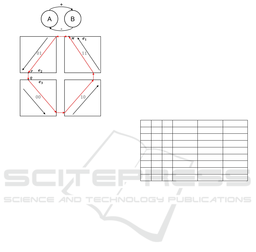
Figure 2: Example of a HGRN of negative feedback loop

with 2 genes: gene A and gene B, where A activates B and

B inhibits A. Abscissa represents the ﬁrst gene (gene A) and

ordinate represents the second gene (gene B).

When a trajectory reaches several output boundaries

at the same time, it can cross any of them but can

only cross one boundary at a time, which causes non-

deterministic behaviors.

2.2 HGRN of the Repressilator

Here we only focus on the inﬂuence graph of the

canonical repressilator, see Figure 1. We assume that

each gene has one threshold when it inﬂuences one

another gene. Although, a priori, one gene can have

multiple thresholds for one another gene, in this work

we only consider the simplest case. Based on this as-

sumption, since each gene only inﬂuences one other

gene in this inﬂuence graph, it has only two discrete

levels separated by only one threshold.

The parameters (celerities) of this HGRN of the

repressilator are shown symbolically in Table 1. Each

parameter in Table 1 is strictly positive and is denoted

by C

xyiz j

, which represents the absolute value of the

celerity of variable x when the discrete level of vari-

able y is i and the discrete level of variable z is j. Con-

sider the inﬂuence of A on B: when the discrete level

of A is 1, meaning that the expression of A is above

the threshold to inhibit B, then the temporal derivative

of B is always negative, no matter the discrete level of

B (0 or 1) which corresponds to the negative values

−C

ba1b0

and −C

ba1b1

. On the other hand, when the

expression of A is below the threshold to inhibit B,

the temporal derivative of B is always positive, cor-

responding to parameters C

ba0b0

and C

ba0b1

. From

the parameters in this table, we can also see that the

number of different parameters (12) is smaller than

the multiplication of the number of dimensions by the

number of discrete states (24), because some discrete

states have celerities in common (same regulation on

some variables).

In addition to the threshold which separates the

discrete levels 0 and 1, each gene also has a maximal

value and a minimal value. For example, when A in-

hibits B (see Figure 1), B will continue to decrease

until it reaches the minimal value (most of the time

this minimal value is 0) which is related to the lower

boundary in the second dimension (the dimension of

gene B) of discrete state 10∗, where ∗ can be 0 or 1.

Similarly, when A does not inhibit B, B will continue

to increase until it reaches the upper boundary in the

second dimension of 01∗.

Table 1: Parameters of the HGRN of the repressilator.

A B C C

0 0 0 C

ac0a0

ba0b0

cb0c0

0 0 1 −C

ac1a0

ba0b0

cb0c1

0 1 0 C

ac0a0

ba0b1

−C

cb1c0

0 1 1 −C

ac1a0

ba0b1

−C

cb1c1

1 0 0 C

ac0a1

−C

ba1b0

cb0c0

1 0 1 −C

ac1a1

−C

ba1b0

cb0c1

1 1 0 C

ac0a1

−C

ba1b1

−C

cb1c0

1 1 1 −C

ac1a1

−C

ba1b1

−C

cb1c1

Figure 3 gives two simulations with two different

choices of parameters. The simulation on the left rep-

resents a sustained oscillation while the simulation on

the right represents a damped oscillation. In the sim-

ulation on the left, gene C continues to increase from

t = 0 until it reaches the maximal value, which also

means that the trajectory reaches an attractive bound-

ary, then the trajectory will slide along this boundary

(called the sliding mode) so that the value of gene C

stays unchanged for some time. The sliding mode is

an important property of HGRNs.

3 QUALITATIVE BEHAVIORS IN

THIS HGRN OF THE

REPRESSILATOR

In this section, we discuss different qualitative prop-

erties of this HGRN. To analyze dynamical proper-

ties of a HGRN, we need to ﬁrstly analyze the transi-

tion graph of discrete states, which is determined by

the signs of celerities. The signs of celerities of this

HGRN of the repressilator can be found in Table 1,

based on which the transition graph of discrete states

can be constructed using the classical discrete asyc-

BIOINFORMATICS 2023 - 14th International Conference on Bioinformatics Models, Methods and Algorithms

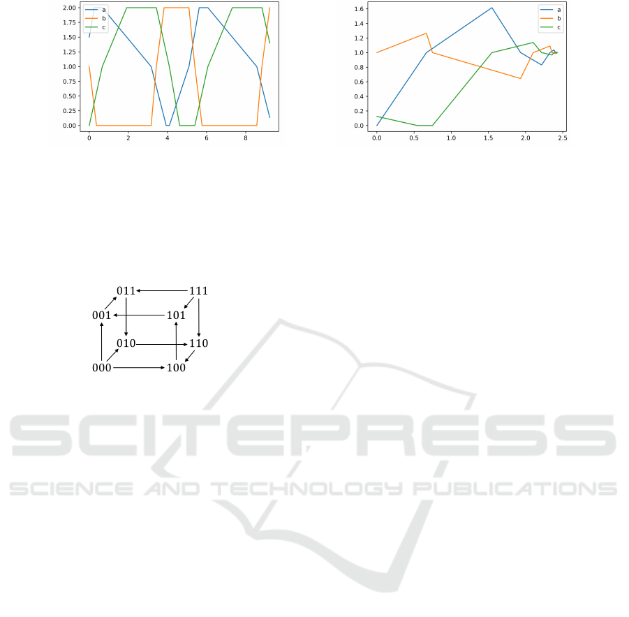
Figure 3: Simulations of the HGRN of the repressilator with two different choices of parameters (Abscissa represents time

and ordinate represents the sum of the fractional part and the discrete state of each gene). Parameters of the model on

the left: C

ac0a0

= 1, C

ac0a1

= 1.9, C

ac1a0

= 1.3, C

ac1a1

= 0.4, C

ba0b0

= 3.8, C

ba0b1

= 2.5, C

ba1b0

= 2.7, C

ba1b1

= 3.3,

cb0c0

= 1.5, C

cb0c1

= 0.8, C

cb1c0

= 1.9, C

cb1c1

= 1.5. Parameters of the model on the right: C

ac0a0

= 1.5, C

ac0a1

= 0.7,

ac1a0

= 0.6, C

ac1a1

= 1.6, C

ba0b0

= 2.1, C

ba0b1

= 0.4, C

ba1b0

= 0.3, C

ba1b1

= 3.3, C

cb0c0

= 1.25, C

cb0c1

= 0.25, C

cb1c0

= 0.23,

cb1c1

= 1.23.

nhronous semantics, see Figure 4.

Figure 4: Transition graph of discrete states of the HGRN

of the repressilator.

From the transition graph, we can see that there

is a unique cycle of discrete states, which is 001 −→

011 −→ 010 −→ 110 −→ 100 −→ 101 −→ 001. This cycle

is a global attractor of discrete states (the unique ter-

minal strongly connected component), which means

that any trajectory in this HGRN will ﬁnally enter this

cycle.

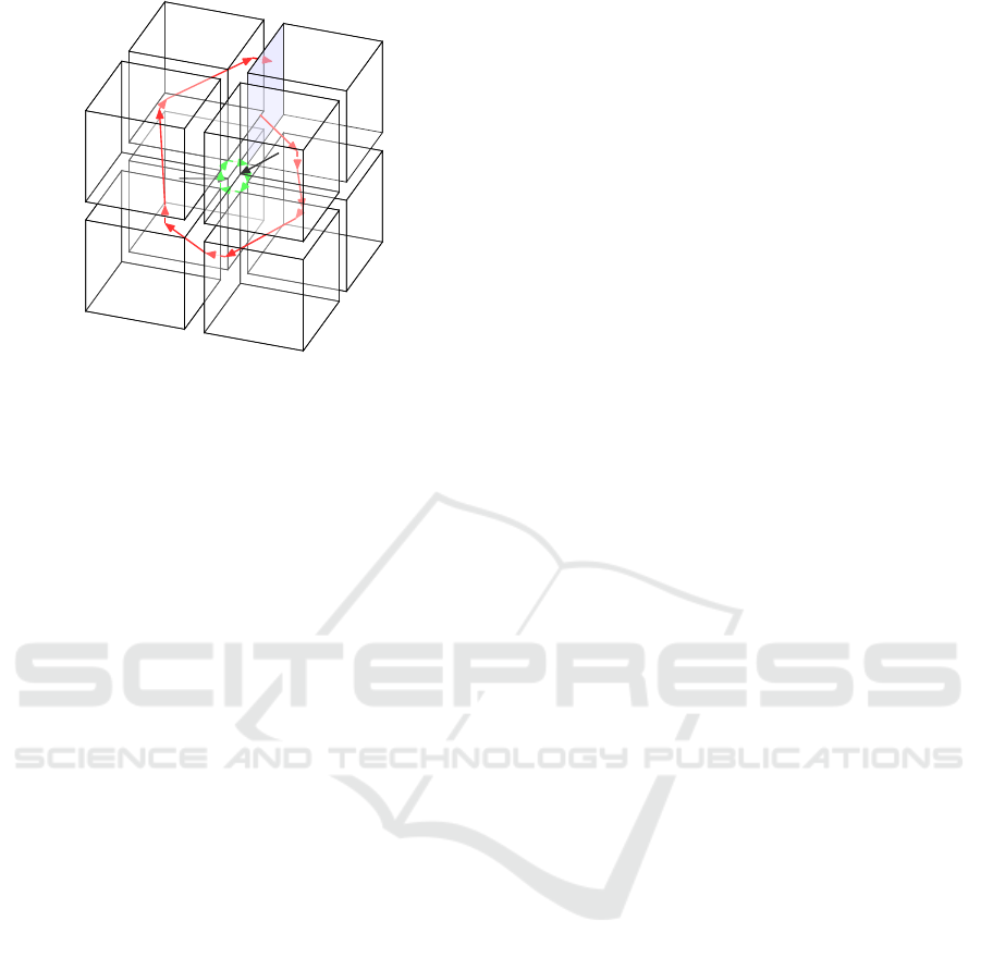
Following the same sequence of discrete

states, there is a special hybrid trajectory:

((1,1, 0),(0, 0,1)) −→ ((1,0, 0),(0, 1,1)) −→

((1,0, 1),(0, 1,0)) −→ ((0,0, 1),(1, 1,0)) −→

((0,1, 1),(1, 0,0)) −→ ((0,1, 0),(1, 0,1)) −→

((1,1, 0),(0, 0,1)). It is illustrated in Figure 5

by green arrows. This trajectory contains 6 different

states (the last and the ﬁrst one are identical). From

each state in this trajectory, there is an instant tran-

sition (transition which crosses boundaries between

discrete states and takes no time), which reaches the

next state. This trajectory represents also a closed

trajectory, meaning that beginning from each of

these 6 states, the trajectory will return to the initial

state. When representing trajectories, we often use

an embedding of hybrid states in R

: a state (π,d

)

is represented in R

by summing its discrete and

fractional parts: π + d

. We say that the hybrid state

(π,d

) and the point π + d

∈ R

are related. When

doing so, the six previous hybrid states are embedded

in the same point H

in R

: H

= (1.0,1.0, 1.0). H

is called a characteristic state of this HGRN. The

characteristic state is formally deﬁned as follows:

Deﬁnition 5 (Characteristic state). A characteristic

state of a HGRN is a state H in the continuous space

such that: for any hybrid state h

related to H, all

trajectories from h

will never reach a hybrid state

which is not related to H, and there exist oscillations

in any small neighborhood of H.

In this paper, we say that a trajectory of a HGRN

is an oscillation if it is related to an oscillation in the

continuous space. Likewise, the nature of an oscilla-

tion of a HGRN (damped or sustained) and the rela-

tion between an oscillation and a characteristic state

(converging to the characteristic state, moving away

from it, etc.) are determined by the related oscilla-

tion in the continuous space. A neighborhood of a

characteristic state H is deﬁned as a set N (H) =

{

(π,d

) ∈ E

| ∥π + d

− H∥ < r

}

where r ∈ R is the

radius of the neighborhood.

In the continuous space, a characteristic state is a

ﬁxed point, because from any hybrid state h related

to a characteristic state, all trajectories can only reach

hybrid states related to this characteristic state.

We can easily prove that H

is a characteristic

state: apart from the 6 hybrid states on this closed tra-

jectory, there are two other hybrid states which are re-

lated to H

: ((1,1, 1),(0,0,0)) and ((0,0,0), (1,1, 1))

From each of these two other states, all trajectories

reach directly the closed trajectory, and once they do,

they can never leave it. Finally, we can ﬁnd oscilla-

tions which follow the unique cycle of discrete states

in any neighborhood of H

. In this HGRN, there is

only one characteristic state. This can be proved by

verifying all “corners” of discrete states.

All trajectories in this HGRN will oscillate in this

unique cycle of discrete states, except some special

trajectories from discrete state 000 or 111 which can

reach directly a hybrid state related to the characteris-

Condition for Sustained Oscillations in Repressilator Based on a Hybrid Modeling of Gene Regulatory Networks

000

100

010

001

011

101

110

111

Figure 5: Illustration of the closed trajectory with only

instant transitions (green arrows), two special trajectories

which can reach directly the characteristic state (black ar-

rows), and a trajectory without sliding mode (red arrows) in

this HGRN of the canonical repressilator.

tic state, see for example the black arrows in Figure 5.

These oscillations can have several different dynami-

cal properties.

To better illustrate the possible dynamical prop-

erties in this repressilator, different qualitative behav-

iors of a HGRN of negative feedback loop in 2 dimen-

sions are illustrated in Figure 6, where black arrows

represent celerities in each discrete state and red ar-

rows represent some trajectories. The three ﬁgures

are obtained by choosing three different parameteri-

sations, which represent the three qualitative behav-

iors of this HGRN. The closed trajectory with states

P,M,N, Q contains only instant transitions. The state

in continuous space that is related to states P,M,N, Q

is a characteristic state, and is the only characteris-

tic state in this HGRN. On the left, the characteristic

state is stable as all trajectories tend to converge to it.

In this case, there is no sustained oscillation. On the

right, the characteristic state is unstable as all trajec-

tories from a small neighborhood of the characteristic

state will move away from it and will ﬁnally reach a

stable limit cycle containing at least one sliding mode,

like the closed trajectory in Figure 2. Between these

two cases, in the middle, there is a third possibility in

which all trajectories circle around the characteristic

state without getting closer or moving away, which we

call parallel cycles and can be considered as a special

case of sustained oscillations.

The HGRN of the repressilator in 3 dimensions

(Figure 1) is more complicated than the example

HGRN of negative feedback loop in 2 dimensions

(Figures 2 and 6), but we think that it also has three

similar qualitative behaviors, since each discrete state

in the only cycle of discrete states has only one suc-

cessor (Figure 4). However, we have no proof for the

non-existence of other possibilities yet, for example

chaos or the co-existence of sustained oscillations and

a stable ﬁxed point. So in this work, we make Hypoth-

esis 1.

Hypothesis 1. In this HGRN of canonical repressila-

tor (see Figure 1 and Table 1), either the characteris-

tic state is stable and all oscillations are damped, or

the characteristic state is unstable and all oscillations

are sustained.

In this HGRN of the canonical repressilator, the

characteristic state is said stable if we can ﬁnd a small

neighborhood around the characteristic state such that

all oscillations which begin from this neighborhood

converge to the characteristic state, and the character-

istic state is said unstable if there is no damped oscil-

lation which converges to it.

Now, based on Hypothesis 1, we can use the sta-

bility of the characteristic state to determine the ex-

istence of sustained oscillations in this HGRN of the

repressilator: all oscillations are sustained if and only

if the characteristic state is unstable. This is the main

idea used in this work to ﬁnd conditions for the ex-

istence of sustained oscillations. A similar idea was

used in other works with differential models, see for

example (Page and Perez-Carrasco, 2018; Wang et al.,

2006; El Samad et al., 2005).

The problem now is how to analyze the stability of

the characteristic state. To do so, we apply a method

based on the Poincar

e map.

4 ANALYSIS OF THE POINCAR

MAP

In this section, a method based on the Poincar

e map is

proposed to compute a sufﬁcient and necessary con-

dition for the existence of sustained oscillations.

4.1 Poincar

e Map in HGRNs

The Poincar

e map was initially proposed to study

limit cycles of nonlinear dynamical systems and has

also been used later to study limit cycles of hybrid

systems (Belgacem et al., 2020; Firippi and Chaves,

2020; Znegui et al., 2020; Flieller et al., 2006; Ed-

wards and Glass, 2005; Girard, 2003; Hiskens, 2001;

Edwards, 2000; Mestl et al., 1996). The Poincar

e map

is the intersection of a periodic orbit with a lower di-

mension subspace which is called the Poincar

e sec-

tion. The properties of the periodic orbit can be de-

rived from the Poincar

e map. In the case of the re-

pressilator studied in this paper, the blue boundary in

Figure 5 could be chosen as a Poincar

e section.

BIOINFORMATICS 2023 - 14th International Conference on Bioinformatics Models, Methods and Algorithms

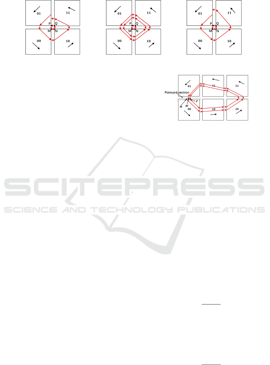
Figure 6: Illustration of different qualitative behaviors in a HGRN of negative feedback loop in 2 dimensions. The three

subﬁgures represent three different choices of parameters.

A method based on the Poincar

e map was pro-

posed in (Sun et al., 2022) to analyze the stability of

limit cycles in HGRNs. To illustrate this method, con-

sider another example in 2 dimensions, with an addi-

tional discrete level in the ﬁrst dimension, as shown

in Figure 7. In this example, we assume that all pa-

rameters (celerities) are known, that is, their real val-

ues can directly be used. The upper boundary in the

second dimension of discrete state 00 is chosen as

Poincar

e section. We can see that there is a closed tra-

jectory which intersects this Poincar

e section at state

P = (π

,(0, 0)), where π

∈ [0, 1]

is the fractional

part of state P. We note that in this particular case,

= (x,1) where x ∈ [0,1], thus there is only one

varying dimension to study in this Poincar

e section.

According to the properties of HGRNs, we can ﬁnd

on the Poincar

e section a neighborhood N around P,

such that trajectory from any state M = (π

,(0, 0))

from N will return to the Poincar

e section at state

′

= (π

′

,(0, 0)) and the relation between π

and

′

can be described by an afﬁne matrix application:

′

= G(π

) = Aπ

+ b (1)

where A is a matrix and b is a vector. We note that

the form of Equation (1) is general and applies to any

case, including those of dimension higher than 2. At

this point, the stability of the closed trajectory de-

pends on the eigenvalues of A. For more details, see

(Sun et al., 2022).

In this work, we adapt this method based on the

Poincar

e map to analyze the stability of the character-

istic state, which is a special case of closed trajectory,

in order to ﬁnd conditions for sustained oscillations.

As opposed to (Sun et al., 2022) where parameters are

assumed to be known, here we compute and analyze

symbolically the Poincar

e map.

4.2 Symbolic Poincar

e Map

In order to analyze the stability of the characteristic

state, we only need to consider trajectories without

sliding mode around this state. Indeed, the charac-

teristic state is stable if we can ﬁnd a small neigh-

borhood around the characteristic state such that all

Figure 7: Illustration of the Poincar

e map in a HGRN.

oscillations which begin from this neighborhood con-

verge to the characteristic state. Such a trajectory ex-

ists because otherwise, the celerities would prevent

the characteristic state from existing. Without loss

of generality, we choose the lower boundary in the

second dimension of discrete state 011 as Poincar

section; see the blue boundary in Figure 5. Now, we

consider any trajectory τ which begins from a state

= ((x

,0, z

),(0, 1,1)) on the Poincar

e section and

returns to the Poincar

e section for the ﬁrst time at

= ((x

,0, z

),(0, 1,1)) without sliding mode; such

a trajectory is illustrated in red in Figure 5. Thus,

the Poincar

e map is an afﬁne application describing

the relation between (x

,0, z

) and (x

,0, z

). Since

is on an input boundary of the discrete state 011,

from s

, τ will ﬁrst (continuously) cross the discrete

state 011 and reach a state ((x

,0), (0,1, 1)) on the

lower boundary in the third dimension of 011 which is

the output boundary of this discrete state towards 010.

We name this output boundary e

. Then, it crosses in-

stantly e

and reaches an input boundary of 010 in

state ((x

,1), (0,1, 0)). The duration of crossing in

discrete state 011 is:

0 − z

−C

cb1c1

(2)

It should be noted that, to ensure that this trajec-

tory τ has no sliding mode in 011, we also need to

ensure that the lower boundary in the ﬁrst dimension

and the upper boundary in the second dimension of

011 are not reached before e

, which gives us two ad-

ditional inequalities:

0 − x

−C

ac1a0

(3)

Condition for Sustained Oscillations in Repressilator Based on a Hybrid Modeling of Gene Regulatory Networks

1 − 0

ba0b1

(4)

In fact, these inequalities can always be satisﬁed if τ

is sufﬁciently close to the characteristic state, which

is the case we consider here. Therefore, in the rest

of this section, we do not consider these additional

constraints.

Based on the duration t

and the fact that there

is no sliding mode, we can get the relation between

,0, z

) and (x

,1):

= x

−C

ac1a0

×t

(5)

= 0 +C

ba0b1

×t

(6)

Following the same process, we can get the du-

ration of τ in each discrete state and the relations be-

tween states from one input boundary to another input

boundary:

1 − x

ac0a0

0 − y

−C

ba1b1

1 − z

cb0c0

(7)

0 − x

−C

ac1a1

1 − y

ba0b0

(8)

= y

ba0b1

×t

= 1 −C

cb1c0

×t

(9)

= 0 +C

ac0a1

×t

= z

−C

cb1c0

×t

(10)

= x

ac0a1

×t

= 1 −C

ba1b0

×t

(11)

= y

−C

ba1b0

×t

= 0 +C

cb0c1

×t

(12)

= 1 −C

ac1a0

×t

= z

cb0c1

×t

(13)

where t

are the durations of τ in dis-

crete states 010, 110, 100, 101, 001 respectively, and

(0,y

),(x

,1, z

),(x

,0), (1,y

),(x

,0, z

)

are the fractional parts of the states when τ ﬁrst

reaches 110, 100, 101, 001, 011 respectively.

Based on the above equations, the Poincar

e map

can be calculated to describe the relation between

,0, z

) and (x

,0, z

) as follows. One dimension is

missing in the matrix below; indeed, this dimension

is useless in the computation of the stability, for more

details see (Sun et al., 2022).















(14)

In the above equation, a

, a

, b

, c

are nonlin-

ear combinations of the celerity values. Their expres-

sions are given in Supplementary Material Section 1.

We can easily derive that b

and c

are strictly posi-

tive, while b

and c

are strictly negative.

4.3 Analysis of Eigenvalues

The stability of the characteristic state depends on the

two eigenvalues of





, which are:

+ c

− c

)

+ 4c

(15)

+ c

−

− c

)

+ 4c

(16)

Property 1. These two eigenvalues are real and

strictly positive.

The proof of Property 1 is given in Supplementary

Material Section 3.

Suppose that two eigenvectors which are related

to λ

and λ

respectively are v

= (v

) and v

). We have the following property on v

and v

Property 2. v

× v

< 0 and v

× v

> 0.

The proof of Property 2 is given in Supplementary

Material Section 4.

Based on these properties, we develop the follow-

ing theorem to verify the stability of the characteristic

state.

Theorem 1. The characteristic state is unstable if

and only if λ

≥ 1.

The proof of Theorem 1 is given in Supplementary

Material Section 5.

Based on Hypothesis 1 and Theorem 1, the condi-

tion λ

≥ 1 is a sufﬁcient and necessary condition for

the existence of sustained oscillations in this HGRN

of canonical repressilator.

Since our ﬁnal objective is to provide practical in-

formation for the construction of synthetic networks,

conditions like λ

≥ 1 might not be a good result,

because the set of models under this constraint is

not easy to ﬁgure. In the next section, a method to

compute separable constraints based on the condition

≥ 1 is presented.

5 COMPUTATION OF

SUFFICIENT SEPARABLE

CONSTRAINTS ON

PARAMETERS

In this section, we propose a method to compute sepa-

rable constraints on parameters based on the condition

≥ 1 which is developed in the previous section.

In this paper, separable constraints mean constraints

with separable form: each parameter is constrained

by an interval, for example C

ac0a0

∈ [C

ac0a0

In other words, these separable constraints represent

a n-dimensional bounding box in the space of param-

eters (celerities). What we want to do is to ﬁnd such a

n-dimensional box so that any model in this bounding

box satisﬁes the condition λ

≥ 1, which means that

any model in this box has sustained oscillations.

Firstly, we present a simpliﬁcation of the condi-

tion λ

≥ 1. Secondly, we introduce a method to ver-

ify if all models in a given bounding box satisfy this

BIOINFORMATICS 2023 - 14th International Conference on Bioinformatics Models, Methods and Algorithms

simpliﬁed condition. At last, using the method in the

second part, we propose a search algorithm to ﬁnd

some separable constraints.

5.1 Condition Simpliﬁcation

The condition:

+ c

− c

)

+ 4c

≥ 1 (17)

can be reformulated as:

+ c

− 2 ≥ −

− c

)

+ 4c

(18)

which is equivalent to:

+ c

− 2 ≥ 0) ∨

((b

+ c

− 2 < 0) ∧

((b

+ c

− 2)

≤ (b

− c

)

+ 4c

))

(19)

or:

+ c

− 2 ≥ 0) ∨ (b

− c

− b

− c

+ 1 ≤ 0)

(20)

This last condition is equivalent to (P

≥ 0)∨(P

≥ 0)

where P

and P

are polynomials on parameters. The

expressions of P

and P

are given in Supplementary

Material Section 2.

Condition (P

≥ 0) ∨ (P

≥ 0) seems preferable

to λ

≥ 1 because it only contains polynomials. In

fact, one can easily prove that solutions for (P

≥

0) ∨ (P

≥ 0) exist. For example, by only consider-

ing Cac0a0 and Cac0a1, which are two parameters

describing the derivative of gene A when gene C does

not inhibit gene A, P

and P

can be expressed by:

×C

ac0a0

+ p

×C

ac0a1

+ p

×C

ac0a0

×C

ac0a1

+ p

(21)

×C

ac0a0

+ p

×C

ac0a1

+ p

×C

ac0a0

×C

ac0a1

+ p

(22)

where p

i j

(with i ∈

{

1,2

}

, j ∈

{

1,2, 3,4

}

) are expres-

sions of parameters which do not include C

ac0a0

and

ac0a1

. We can see that if C

ac0a0

and C

ac0a1

converge

to 0 while other parameters remain unchanged, P

and P

converge to p

and p

respectively, which

are both positive. This indicates that the solutions

of (P

≥ 0) ∨ (P

≥ 0) exist and also implies a new

control strategy for the existence of sustained oscil-

lations: controlling the derivatives of gene A when

A is not inhibited by C such that these derivatives are

sufﬁciently small, while keeping other parameters un-

changed.

5.2 Satisﬁability Under Separable

Constraints

In this subsection, we adapt the range enclosure prop-

erty of Bernstein coefﬁcients to verify if all models

in a given bounding box satisfy the condition (P

≥

0) ∨ (P

≥ 0). The Bernstein coefﬁcients have been

used in the literature to, for example, compute images

for polynomial dynamical system (Dang and Salinas,

2009; Dang and Testylier, 2012), or compute afﬁne

lower bound functions for polynomials (Garloff and

Smith, 2003), etc.

Before introducing the Bernstein coefﬁcients, we

ﬁrstly introduce the notion of multi-indice. A multi-

indice is a vector of non-negative integers. Given two

multi-indice i = (i

,..., i

) and j = ( j

, j

,..., j

we write i ≤ j if ∀k ∈

{

1,2, ...,n

}

, i

≤ j

. We

also write

for (

,...,

) and





for









...





which is the multiplication of all bi-

nomial coefﬁcient





, k ∈

{

1,2, ...,n

}

Using the multi-indice, a polynomial f : R

→ R

can be represented as follows:

f (x) =

∑

i∈I

(23)

where a

∈ R, i and d are multi-indices, I

is set of

all multi-indices i such that i ≤ d, and x

= x

...x

which is the product of all x

, where x

is the j

vari-

able of polynomial f .

f can also be expressed by Bernstein expansion as

follows:

f (x) =

∑

i∈I

d,i

(x) (24)

where

d,i

(x) = β

)...β

) (25)

) =





(1 − x

)

−i

(26)

∑

j≤i









(27)

where d and i are multi-indices and k ∈

{

1,2, ...,n

}

The values b

, for i ∈ I

are called Bernstein coefﬁ-

cients.

One fundamental property of Bernstein coefﬁ-

cients for our approach is the range enclosure prop-

erty, which can be derived from the convex hull prop-

erty. The convex hull of a set S, noted Conv(S), is the

smallest convex set that contains S.

Condition for Sustained Oscillations in Repressilator Based on a Hybrid Modeling of Gene Regulatory Networks

Lemma 1 (Convex hull property).

Conv

{

(x, f (x)) | x ∈ B

}

⊆ Conv

{

(i/d, b

) | i ∈ I

}

Lemma 2 (Range enclosure property).

min

{

| i ∈ I

}

≤ f (x) ≤ max

{

| i ∈ I

}

, ∀x ∈ B,

where B = [0, 1]

is the unit box.

The range enclosure property over-approximates

the range of image of f on B and can be used to verify

if all models in a given bounding box satisfy the con-

dition (P

≥ 0) ∨(P

≥ 0). To do so, we need to ﬁrstly

make a change of variables of polynomials P

and P

such that all variables are included in [0,1]. For exam-

ple, the variable C

ac0a0

∈ [C

ac0a0

] is replaced

by C

ac0a0

= (C

ac0a0

−C

ac0a0

)× X

ac0a0

, where

ac0a0

∈ [0,1]. By doing so, we get two new polyno-

mials P

′

and P

′

So now, to verify if (P

≥ 0) ∨ (P

≥ 0) is always

true in a given bounding box, we only need to ver-

ify if (P

′

≥ 0) ∨ (P

′

≥ 0) is always true in the unit

box. To do so, we compute the Bernstein coefﬁ-

cients

{

1,i

}

and

{

2,i

}

(where i ∈ I

) of P

′

and P

′

respectively. A sufﬁcient condition for the condition

“(P

′

≥ 0) ∨ (P

′

≥ 0) is always true in the unit box”

(condition1) is “(∀i ∈ I

, b

1,i

≥ 0) ∨ (∀i ∈ I

, b

2,i

≥ 0)”

(condition2), according to the range enclosure prop-

erty. In fact, since the minimum value of the image

of P

′

on the unit box is always larger or equal to the

minimum value of

{

1,i

}

, “

{

1,i

}

are not negative”

(∀i ∈ I

, b

1,i

≥ 0) indicates that “P

′

are not negative on

the unit box”, and the same holds for P

′

. Since there is

a ﬁnite number of Bernstein coefﬁcients, condition2

can be veriﬁed. Therefore, in this work, condition2 is

used to verify if all models in a given bounding box

always have sustained oscillations.

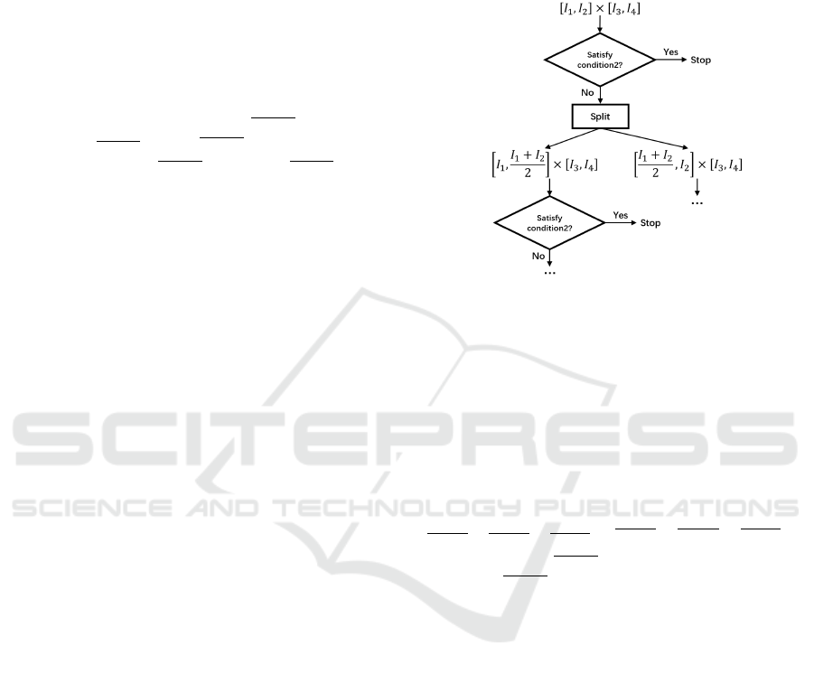
5.3 Search of Separable Constraints

Based on the method introduced in the previous sub-

section, we propose a depth ﬁrst algorithm to ﬁnd

some bounding boxes which satisfy condition2. This

algorithm is illustrated in Figure 8. Initially, each pa-

rameter is included in an interval. In this implementa-

tion, without loss of generality, we assume that each

parameter is included initially in [0, 1]. Then, we ver-

ify if condition2 is satisﬁed for this bounding box us-

ing the method proposed in the previous subsection.

If it is satisﬁed, then it is a bounding box such that all

models in it have sustained oscillations. If condition2

is not satisﬁed, then there might be some models in

this bounding box which do not have sustained oscil-

lations, in this case the bounding box is split into two

smaller bounding boxes (by splitting the largest in-

terval into two) which have the same volume and the

process is repeated on each of these two new bound-

ing boxes. Each path in this algorithm will stop, ei-

ther when a bounding box which satisﬁes condition2

is found or when the length of the largest interval is

smaller than a certain threshold. In fact, similar ideas

are widely used to ﬁnd solution sets under non-linear

constraints (Ziat et al., 2019; Pelleau et al., 2013).

Figure 8: Illustration of the algorithm to search for some

bounding boxes.

Since the HGRN of the canonical repressilator has

12 parameters (see Table 1), and if we assume that

the number of possible smallest intervals for each pa-

rameter are the same, noted m, then there are at most

smallest bounding boxes to check. Verifying all

these boxes can be time consuming. In our imple-

mentation, we assume that the intervals of these three

genes are identical, which means that we search for

bounding boxes such that C

acia j

= C

baib j

= C

cbic j

and

acia j

= C

baib j

= C

cbic j

for any i, j ∈

{

0,1

}

, where, for

example, [C

ac0a0

] is the interval of the param-

eter C

ac0a0

, so that we only need to consider 4 inde-

pendent intervals when searching for bounding boxes.

This assumption is only applied here to decrease the

number of possible bounding boxes. Similar assump-

tion about the symmetry between these three genes

was also made in works based on differential equa-

tions, see for example (Bus¸e et al., 2010). We also

assume that the minimal length of interval is greater

or equal to 0.5. A value smaller than 0.5 could natu-

rally be chosen, but this might exponentially increase

the number of possible bounding boxes, which could

also exponentially increase the execution time. With

these assumptions, we obtain 5 bounding boxes which

satisfy the condition2. In the results below, (y,x) rep-

resents (c, a), (a,b) and (b,c), where y inhibits x, for

example C

xy0x0

presents C

ac0a0

, C

ba0b0

and C

cb0c0

Bounding box 1: C

xy0x0

∈ [0,0.5],C

xy0x1

∈

[0,0.5],C

xy1x0

∈ [0.5, 1],C

xy1x1

∈ [0, 1]

Bounding box 2: C

xy0x0

∈ [0,0.5],C

xy0x1

∈

[0.5,1],C

xy1x0

∈ [0, 0.5],C

xy1x1

∈ [0, 0.5]

Bounding box 3: C

xy0x0

∈ [0,0.5],C

xy0x1

∈

BIOINFORMATICS 2023 - 14th International Conference on Bioinformatics Models, Methods and Algorithms

[0.5,1],C

xy1x0

∈ [0.5, 1],C

xy1x1

∈ [0, 1]

Bounding box 4: C

xy0x0

∈ [0.5,1],C

xy0x1

∈

[0.5,1],C

xy1x0

∈ [0, 0.5],C

xy1x1

∈ [0, 0.5]

Bounding box 5: C

xy0x0

∈ [0.5,1],C

xy0x1

∈

[0.5,1],C

xy1x0

∈ [0.5, 1],C

xy1x1

∈ [0, 1]

We can see that these constraints are easy to in-

terpret and some intuitive results can be derived from

them: for instance, from Bounding box 2, we can get

that sustained oscillations exist if the values of C

xy0x1

are close to each other and are sufﬁciently larger than

any C

xy0x0

, C

xy1x0

and C

xy1x1

6 CONCLUSIONS

In this work, a HGRN of the canonical repressila-

tor is constructed. By computing and analyzing an-

alytically a Poincar

e map and based on a hypothe-

sis, a sufﬁcient and necessary condition for the ex-

istence of sustained oscillations is developed. Then

the range enclosure property of Bernstein coefﬁcients

is adapted to ﬁnd some bounding boxes in parame-

ters space which satisfy this sufﬁcient and necessary

condition. These bounding boxes (intervals of param-

eters) can provide useful information for the design

of synthetic circuits. Moreover, an intermediate re-

sult implies some new control strategies for sustained

oscillations: controlling the absolute values of the

derivatives of one gene under certain regulation such

that these values are sufﬁciently small, while keeping

other parameters of the system unchanged.

Naive assumptions about the bounding boxes are

made in this work. For example, we assume that

the inﬂuence between these three genes are symmetri-

cal. In other words, some groups of parameters (such

as C

ac0a0

, C

ba0b0

and C

cb0c0

) are constrained by the

same intervals. These assumptions could be replaced

by more realistic ones with access to more biologi-

cal knowledge. For instance, knowing the intervals of

possible values for some parameters would allow to

speed up the enumeration of the bounding boxes.

Only the canonical repressilator with three com-

ponents is considered in this work. This method could

be extended for more complex inﬂuence graphs that

exist in the literature (Page, 2019; Perez-Carrasco

et al., 2018; Goh et al., 2008). However, for more

complex inﬂuence graphs, conditions for the exis-

tence of sustained oscillations can be harder to de-

velop, as there could be several cycles of discrete

states around one characteristic state: in such a case,

one would have to consider the disjunction of the con-

ditions associated with each cycle. It is also possible

to extend this work to ﬁnd condition for other dynam-

ical properties expressed with temporal logics.

In this work, constraints are obtained based on

given dynamical properties. In future works, the con-

verse approach might be considered, that is, given a

bounding box of parameters, predict possible behav-

iors of the system.

ACKNOWLEDGEMENTS

We would like to thank Gilles Bernot and Thao Dang

for their fruitful discussions.

This work is partly supported by China Scholar-

ship Council.

ADDITIONAL INFORMATION

Supplementary Material is available at https://hal.

archives-ouvertes.fr/hal-03890505/document. The

code of this work is available at https://github.com/

Honglu42/HGRN repressilator.

REFERENCES

Batt, G., Belta, C., and Weiss, R. (2007). Model check-

ing genetic regulatory networks with parameter uncer-

tainty. In International Workshop on Hybrid Systems:

Computation and Control, pages 61–75. Springer.

Behaegel, J., Comet, J.-P., Bernot, G., Cornillon, E., and

Delaunay, F. (2016). A hybrid model of cell cycle in

mammals. Journal of bioinformatics and computa-

tional biology, 14(01):1640001.

Belgacem, I., Gouz

e, J.-L., and Edwards, R. (2020). Control

of negative feedback loops in genetic networks. In

2020 59th IEEE Conference on Decision and Control

(CDC), pages 5098–5105. IEEE.

Bus¸e, O., Kuznetsov, A., and P

erez, R. A. (2009). Ex-

istence of limit cycles in the repressilator equa-

tions. International Journal of Bifurcation and Chaos,

19(12):4097–4106.

Bus¸e, O., P

erez, R., and Kuznetsov, A. (2010). Dynamical

properties of the repressilator model. Physical Review

E, 81(6):066206.

Chaves, M. and Gouz

e, J.-L. (2011). Exact control of ge-

netic networks in a qualitative framework: the bistable

switch example. Automatica, 47(6):1105–1112.

Chaves, M. and Jong, H. d. (2021). Qualitative modeling,

analysis and control of synthetic regulatory circuits.

Synthetic Gene Circuits, pages 1–40.

Cornillon, E., Comet, J.-P., Bernot, G., and En

ee, G. (2016).

Hybrid gene networks: a new framework and a soft-

ware environment. advances in Systems and Synthetic

Biology.

Dang, T. and Salinas, D. (2009). Image computation for

polynomial dynamical systems using the bernstein ex-

Condition for Sustained Oscillations in Repressilator Based on a Hybrid Modeling of Gene Regulatory Networks

pansion. In International Conference on Computer

Aided Veriﬁcation, pages 219–232. Springer.

Dang, T. and Testylier, R. (2012). Reachability analysis

for polynomial dynamical systems using the bernstein

expansion. Reliab. Comput., 17(2):128–152.

De Jong, H., Geiselmann, J., Hernandez, C., and Page, M.

(2003). Genetic network analyzer: qualitative simu-

lation of genetic regulatory networks. Bioinformatics,

19(3):336–344.

Dil

ao, R. (2014). The regulation of gene expression in eu-

karyotes: bistability and oscillations in repressilator

models. Journal of theoretical biology, 340:199–208.

Dukari

c, M., Errami, H., Jerala, R., Lebar, T., Romanovski,

V. G., T

oth, J., and Weber, A. (2019). On three genetic

repressilator topologies. Reaction Kinetics, Mecha-

nisms and Catalysis, 126(1):3–30.

Edwards, R. (2000). Analysis of continuous-time switching

networks. Physica D: Nonlinear Phenomena, 146(1-

4):165–199.

Edwards, R. and Glass, L. (2005). A calculus for relating

the dynamics and structure of complex biological net-

works. Adventures in Chemical Physics: A Special

Volume of Advances in Chemical Physics, 132:151–

178.

El Samad, H., Del Vecchio, D., and Khammash, M. (2005).

Repressilators and promotilators: Loop dynamics in

synthetic gene networks. In Proceedings of the 2005,

American Control Conference, 2005., pages 4405–

4410. IEEE.

Elowitz, M. B. and Leibler, S. (2000). A synthetic oscil-

latory network of transcriptional regulators. Nature,

403(6767):335–338.

Firippi, E. and Chaves, M. (2020). Topology-induced

dynamics in a network of synthetic oscillators with

piecewise afﬁne approximation. Chaos: An Interdisci-

plinary Journal of Nonlinear Science, 30(11):113128.

Flieller, D., Riedinger, P., and Louis, J.-P. (2006). Compu-

tation and stability of limit cycles in hybrid systems.

Nonlinear Analysis: Theory, Methods & Applications,

64(2):352–367.

Garloff, J. and Smith, A. P. (2003). A comparison of

methods for the computation of afﬁne lower bound

functions for polynomials. In International Workshop

on Global Optimization and Constraint Satisfaction,

pages 71–85. Springer.

Girard, A. (2003). Computation and stability analysis of

limit cycles in piecewise linear hybrid systems. IFAC

Proceedings Volumes, 36(6):181–186.

Goh, K.-I., Kahng, B., and Cho, K.-H. (2008). Sustained

oscillations in extended genetic oscillatory systems.

Biophysical Journal, 94(11):4270–4276.

Hiskens, I. A. (2001). Stability of hybrid system limit cy-

cles: Application to the compass gait biped robot. In

Proceedings of the 40th IEEE Conference on Decision

and Control (Cat. No. 01CH37228), volume 1, pages

774–779. IEEE.

Kuznetsov, A. and Afraimovich, V. (2012). Heteroclinic

cycles in the repressilator model. Chaos, Solitons &

Fractals, 45(5):660–665.

Mestl, T., Lemay, C., and Glass, L. (1996). Chaos in high-

dimensional neural and gene networks. Physica D:

Nonlinear Phenomena, 98(1):33–52.

uller, S., Hofbauer, J., Endler, L., Flamm, C., Widder,

S., and Schuster, P. (2006). A generalized model of

the repressilator. Journal of mathematical biology,

53(6):905–937.

Page, K. M. (2019). Oscillations in well-mixed, determinis-

tic feedback systems: Beyond ring oscillators. Journal

of Theoretical Biology, 481:44–53.

Page, K. M. and Perez-Carrasco, R. (2018). Degradation

rate uniformity determines success of oscillations in

repressive feedback regulatory networks. Journal of

the Royal Society Interface, 15(142):20180157.

Pelleau, M., Min

e, A., Truchet, C., and Benhamou, F.

(2013). A constraint solver based on abstract do-

mains. In International Workshop on Veriﬁcation,

Model Checking, and Abstract Interpretation, pages

434–454. Springer.

Perez-Carrasco, R., Barnes, C. P., Schaerli, Y., Isalan, M.,

Briscoe, J., and Page, K. M. (2018). Combining a tog-

gle switch and a repressilator within the ac-dc circuit

generates distinct dynamical behaviors. Cell systems,

6(4):521–530.

Potvin-Trottier, L., Lord, N. D., Vinnicombe, G., and Pauls-

son, J. (2016). Synchronous long-term oscillations in

a synthetic gene circuit. Nature, 538(7626):514–517.

Sun, H., Folschette, M., and Magnin, M. (2022). Limit

cycle analysis of a class of hybrid gene regulatory

networks. In International Conference on Computa-

tional Methods in Systems Biology, pages 217–236.

Springer.

Thomas, R. (1973). Boolean formalization of genetic

control circuits. Journal of theoretical biology,

42(3):563–585.

Thomas, R. (1991). Regulatory networks seen as asyn-

chronous automata: a logical description. Journal of

theoretical biology, 153(1):1–23.

Wang, R., Chen, L., and Aihara, K. (2006). Construction

of genetic oscillators with interlocked feedback net-

works. Journal of theoretical biology, 242(2):454–

463.

Ziat, G., Mar

echal, A., Pelleau, M., Min

e, A., and Truchet,

C. (2019). Combination of boxes and polyhedra ab-

stractions for constraint solving. In International Sym-

posium on Formal Methods, pages 119–135. Springer.

Znegui, W., Gritli, H., and Belghith, S. (2020). Design of an

explicit expression of the poincar

e map for the passive

dynamic walking of the compass-gait biped model.

Chaos, Solitons & Fractals, 130:109436.

BIOINFORMATICS 2023 - 14th International Conference on Bioinformatics Models, Methods and Algorithms