Robust Path Planning in the Wild for Automatic Look-Ahead Camera

Control

Sander R. Klomp

1,2 a

and Peter H. N. de With

1 b

Department of Electrical Engineering, Eindhoven University of Technology, Eindhoven, The Netherlands

ViNotion B.V., Eindhoven, The Netherlands

Keywords:

Semantic Segmentation, Deep Learning, Road Segmentation, Path Planning.

Abstract:

Finding potential driving paths on unstructured roads is a challenging problem for autonomous driving and

robotics applications. Although the rise of autonomous driving has resulted in massive public datasets, most

of these datasets focus on urban environments and feature almost exclusively paved roads. To circumvent

the problem of limited public datasets of unpaved roads, we combine seven public vehicle-mounted-camera

datasets with a very small private dataset and train a neural network to achieve accurate road segmentation on

almost any type of road. This trained network vastly outperforms networks trained on individual datasets when

validated on our unpaved road datasets, with only a minor performance reduction on the highly challenging

public WildDash dataset, which is mostly urban. Finally, we develop an algorithm to robustly transform these

road segmentations to road centerlines, used to automatically control a vehicle-mounted PTZ camera.

1 INTRODUCTION

Road segmentation and path planning are two essen-

tial components of autonomous driving systems. In

recent years, large performance gains over conven-

tional computer vision-based systems have been real-

ized using deep learning, allowing for self-driving ve-

hicles on most public roads. However, several corner

cases remain in which these well-established meth-

ods cause failures (Grigorescu et al., 2020), especially

when the perception part of the algorithm cannot seg-

ment the drivable surface correctly.

One of the cases where modern neural network-

based solutions struggle with path planning is on un-

structured roads, where a lack of lane markings can

confuse lane detection networks or networks that di-

rectly perform the path-planning task. This prob-

lem is exacerbated by the fact that the large public

datasets for autonomous driving focus on urban en-

vironments where most roads are structured, such as

BDD100k (Yu et al., 2020) and Cityscapes (Cordts

et al., 2016). The Mapillary Vistas (Neuhold et al.,

2017) and IDD datasets (Varma et al., 2019) include

some types of unstructured roads, but limit their vari-

ation to paved roads. For robust path planning in any

environment, we argue that unpaved roads, such as

https://orcid.org/0000-0002-0874-4720

https://orcid.org/0000-0002-7639-7716

sand, dirt or even just tire tracks, should be included

also.

This research focuses on developing a robust path-

planning system for any type of road. The road seg-

mentation is performed using a HRNetV2-W48 net-

work (Sun et al., 2019) trained on a combination

of eight different datasets, in order to maximize the

variation of learned road types. Additional post-

processing is introduced on the road segmentations

to further improve the robustness. Because existing

datasets are not annotated with paths, we fall back

to a conventional computer vision approach to per-

form the ﬁnal path planning, which is consequently

based on the segmentation masks. Whereas most

of the algorithms in this paper can be also applied

to autonomous driving, the more speciﬁc use case

for which this work has been performed, is differ-

ent. Our main use case is a person-driven vehicle

with a mounted Pan-Tilt-Zoom (PTZ) camera, where

the camera view should automatically stay concen-

trated at the center of the road at a certain distance

in front of the vehicle, thereby actively following any

curves in the road. Several design decisions in the

path-planning algorithm are speciﬁc to this use case,

though most of the algorithms may also be applied

for collision avoidance. Some example outputs of the

algorithm are shown in Fig. 1.

Our contributions are summarized as follows.

1. We combine several urban and non-urban datasets

Klomp, S. and N. de With, P.

Robust Path Planning in the Wild for Automatic Look-Ahead Camera Control.

DOI: 10.5220/0011614200003417

In Proceedings of the 18th International Joint Conference on Computer Vision, Imaging and Computer Graphics Theory and Applications (VISIGRAPP 2023) - Volume 4: VISAPP, pages

553-561

ISBN: 978-989-758-634-7; ISSN: 2184-4321

 2023 by SCITEPRESS – Science and Technology Publications, Lda. Under CC license (CC BY-NC-ND 4.0)

553

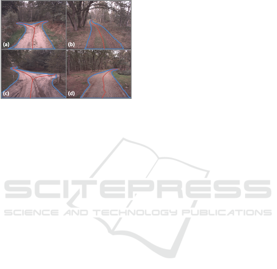
Figure 1: Pathﬁnding examples. Road segmentations are

outlined in blue, estimated centerlines in red.

into a diverse, new large dataset, to maximize the

robustness of a trained segmentation network, al-

lowing it to segment nearly any type of road.

2. A novel path-planning algorithm is developed that

transforms the road segmentation into road cen-

terlines, to be used to control a forward-looking

vehicle-mounted PTZ camera.

2 RELATED WORK

The path-planning system has related work in both

neural networks for semantic segmentation and gen-

eral path planning, which are discussed separately.

2.1 Semantic Segmentation

Early semantic segmentation research using neural

networks, such as the FCN (Shelhamer et al., 2016),

focused on general object segmentation. Since then,

two main improved architectures have become pop-

ular: the encoder-decoder structure with skip con-

nections, popularized by the U-net (Ronneberger

et al., 2015), and the structures that maintain high-

resolution features throughout the entire network,

such as HRNet (Sun et al., 2019). Both types of net-

works reach state-of-the-art performance on various

semantic segmentation datasets.

With the emerging application of autonomous

driving, more public driving segmentation datasets

have become available. These datasets include

Cityscapes (Cordts et al., 2016), IDD (Varma et al.,

2019), BDD100K (Yu et al., 2020) and Mapillary Vis-

tas (Neuhold et al., 2017), which all focus on segmen-

tation in urban environments.

Many works focus on achieving the highest pos-

sible accuracy on these public urban datasets, but

we are interested speciﬁcally in generalizing perfor-

mance on non-urban settings with unstructured roads.

Several works do focus on the detection of unstruc-

tured roads, such as (Nakagomi et al., 2021), (Ya-

dav et al., 2017), (Giusti et al., 2016), (Valada et al.,

2016), but they either require LIDAR (Nakagomi

et al., 2021), use heuristics that are sensitive to color

differences on the road such as shadows (Yadav et al.,

2017), or train on a small dataset with very little

road variation ((Giusti et al., 2016) and (Valada et al.,

2016)). Several datasets also exist containing natu-

ral or rural environments, such as YCOR (Maturana

et al., 2018), RUGD (Wigness et al., 2019), Freiburg

Forest (Valada et al., 2016) and Rellis-3D (Jiang et al.,

2020), but all of these datasets show little variety in

road types and environments. To our knowledge, nei-

ther a comprehensive dataset nor a robust road seg-

mentation method exists yet that yields an acceptable

performance on general unstructured road. Because

of this, our road segmentation will be performed by

training on a combination of the aforementioned un-

paved road datasets.

2.2 Path Planning

For regular autonomous driving, path planning gen-

erally consists of four steps: route planning, behav-

ioral decision-making, motion planning and vehicle

control (Paden et al., 2016). Considering that our

use case is only to control the camera viewing direc-

tion instead of automated driving of the entire vehicle,

most of these steps can be simpliﬁed or even omitted.

“Route planning” is somewhat relevant, because at in-

tersections, the system should choose the correct road

to follow. “Behavioral decision-making” is unneces-

sary, because the human driver determines the route

and the camera does not need to react in any way to

other road users. “Motion planning” involves deter-

mining the detailed path based on the current view of

the road, and is the primary focus of this work. “Ve-

hicle control”, which becomes camera control in our

case, is trivial: rotating a simple PTZ camera is much

simpler than steering a vehicle and does not require

complex vehicle models.

Motion planning can be performed in several

ways. The most straightforward methods are graph

search-based planners, such as the Dijkstra and A* al-

gorithms, although planners based on sampling such

as Rapidly-exploring Random Trees (RRT) are also

common (Gonz

alez et al., 2016). More complex

methods aim to either be faster to compute than A*,

allow for easier integration of other parameters such

as vehicle size, or provide smoother paths which en-

VISAPP 2023 - 18th International Conference on Computer Vision Theory and Applications

554

3.2.1 Road-Mask Processing

3.2.2 Path Planning

Preprocessing

Image inference

Class remapping

Dataset

expansion

Network

training

Connected-

component

filtering

Hole filling

Row-gap filling

Bird’s-eye view

transform

Close-range

filling

Start point

detection

End point(s)

detection

Path finding

Reverse bird’s-

eye transform

3.1 Road Segmentation

Multiple

Datasets

Train time only

Eind point(s)

filtering

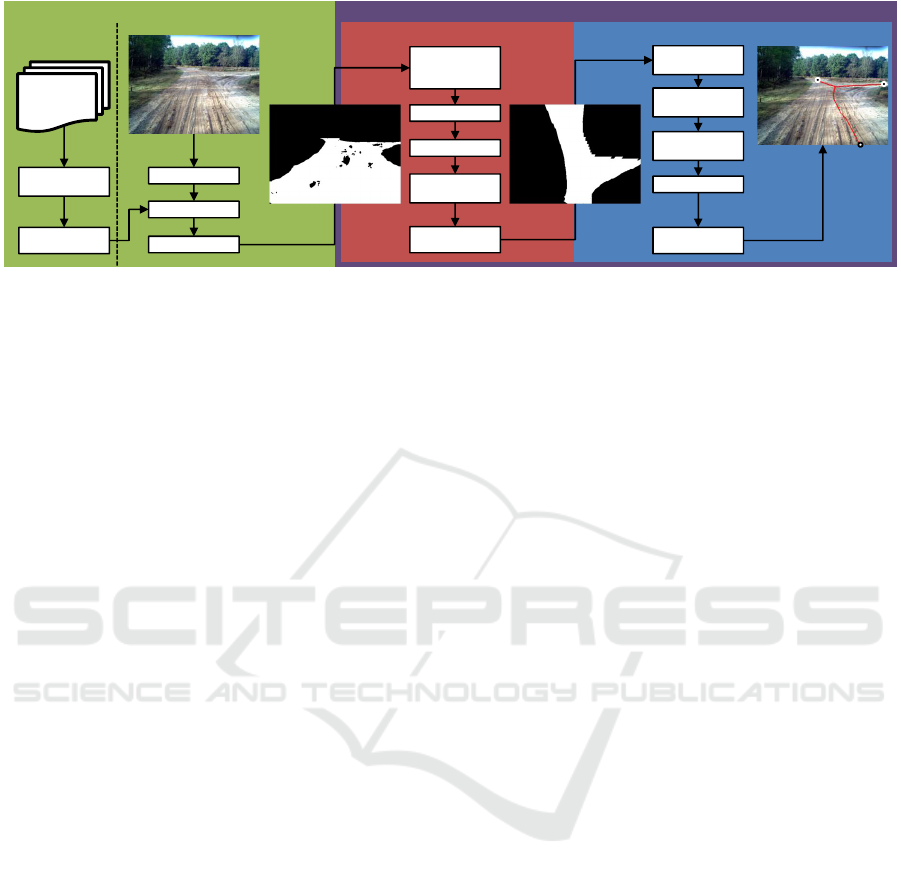
3.2 Robust Path Planning

Figure 2: Flow chart of the path-planning system. Note that a poorly trained network is used deliberately for the segmentation

to highlight the effect of road-mask processing. Road path, start point and end point are shown in the right image.

able smoother vehicle control. For example, motion

planning can be performed far more efﬁciently using a

neural network (Qureshi et al., 2019), by teaching it to

imitate paths generated using RRT. This is especially

useful in high-dimensional spaces and not necessary

for our simple 2D path-planning case. To conclude,

we will perform path planning using the simple A* al-

gorithm, because it is sufﬁciently fast for our use case

and the additional features of more complex methods

are not necessary for camera control.

3 CREATING A ROBUST

PATH-PLANNING SYSTEM

The proposed method consists of three main compo-

nents, as shown in Fig. 2: semantic segmentation,

road-mask processing and path planning. For seman-

tic segmentation, the focus is on how to combine ex-

isting datasets and jointly train on them to achieve

strong generalization. During inference, the seman-

tic segmentation stage simply consists of executing

the network and mapping several classes to a road

mask. The road mask is then post-processed using

multiple conventional computer vision algorithms, to

ensure better pathﬁnding in the ﬁnal stage. Pathﬁnd-

ing itself employs the A* algorithm, although auto-

matically ﬁnding the correct start and end points for

that algorithm is not always straightforward. These

components are now further discussed in detail.

3.1 Road Segmentation: Multi-Dataset

Training for Improved Robustness

This section ﬁrst brieﬂy describes the employed

CNN and the applied training procedure, followed

by an overview of suitable datasets and the proposed

method for combining these datasets.

The base network that is employed for road seg-

mentation is the HRNetV2-W48 network (Sun et al.,

2019). This neural network does not follow the com-

mon encoder-decoder structure, but instead maintains

a full-resolution branch throughout the entire network

and several downsampled branches in parallel for en-

larging the receptive ﬁeld. To ﬁnally combine the

separate branches, the downsampled branches are up-

sampled and concatenated to the main branch (Sun

et al., 2019). Whereas optimizing this architecture

further to improve the robustness of our road segmen-

tation task may be possible, we instead adopt the idea

from MSeg (Grigorescu et al., 2020) and focus on the

data instead of the CNN architecture.

The authors from MSeg have already shown

that an unaltered HRNetV2 trained on seven differ-

ent datasets simultaneously outperforms robustness-

specialized techniques on the highly challenging and

diverse WildDash (Zendel et al., 2018) test set. How-

ever, Mseg does not yet include datasets with unpaved

roads. Furthermore, while WildDash is highly var-

ied from a weather and environments point of view, it

still primarily focuses on urban scenes, making it less

suited as a test set for our work. Because of this, we

will only employ WildDash to verify generalization

of our trained network to urban scenes.

To perform dataset balancing, we adopt the

method from Mseg: in every training batch an equal

number of images from each dataset is used. For

example, this means that if there is one dataset of

10,000 images and one of 1,000 images, the former

will only be seen by the network once per epoch,

while the latter will be seen ten times per epoch.

The advantage of this approach is that it forces the

network to perform well on all datasets, but the

downside is that it may also cause overﬁtting on

small datasets or datasets with low variety. We expect

overﬁtting on the small datasets to not be a problem,

due to the large number of different datasets that we

Robust Path Planning in the Wild for Automatic Look-Ahead Camera Control

555

will be combining, but this aspect should certainly be

kept in mind when combining fewer datasets.

Dataset Expansion. The training datasets that MSeg

employs are extremely varied: two datasets contain-

ing all kinds of scenes, both indoor and outdoor, with

various objects (COCO and ADE20K), the indoor

segmentation dataset SUN RGBD, and the four driv-

ing datasets Mapillary Vistas, IDD, BDD100K and

Cityscapes. MSeg also tests on highly varied datasets,

but we limit ourselves to the testing of road segmenta-

tion, to achieve stronger performance on our special-

ized task: robust road segmentation on unstructured

and unpaved roads.

A. Public Off-Road Dataset Additions.

Several small segmentation datasets exist that may

contain useful data for unpaved road segmentation.

All datasets are ﬁltered to only contain images with

at least one pixel labeled as “road”. The number of

images left after ﬁltering is given between brackets.

• Yamaha-CMU Off-Road (YCOR) dataset (Matu-

rana et al., 2018): 1,076 (982) labeled images col-

lected at four different locations using a vehicle-

mounted camera, with quite variable road types:

concrete, dirt, gravel and tire tracks, providing a

good baseline for unpaved road segmentation.

• Robot Unstructured Driving Ground (RUGD)

dataset (Wigness et al., 2019): 7,453 (3,637) la-

beled images in eight different terrains, recorded

using a small robot. The dataset contains mostly

asphalt and some gravel roads. However, the

roads are clearly not the focus of the data collec-

tion, as the robot mostly drives besides the roads

and paths. The size of the robot also causes the

camera to be very close to the ground.

• Freiburg Forest (FF) dataset (Valada et al., 2016):

366 (366) labeled images in forest environments,

recorded using both an infrared camera and a reg-

ular RGB camera. This data are highly relevant

to our use case, even though the set is relatively

small and contains limited variety. Most roads in

the dataset are gravel-like.

• Rellis-3D dataset (Jiang et al., 2020): A dataset

with 6,235 (3,906) images, recorded in a grass

ﬁeld with dirt tire tracks. Although the dataset is

quite large, the image variety is extremely limited.

We remap all the labels of these four datasets and

combine them with the four public urban driving

datasets, for a total of eight different training datasets.

B. Semi-Supervised Addition of New Data

To increase the variety of data further, additional

data are recorded and annotated. Data are recorded

on several road types: sand, dirt, tire tracks, as-

phalt, concrete and stone-paved roads, mostly in for-

est environments. Since the focus is on road seg-

mentation and the creation of full-image semantic la-

bels is extremely time-consuming, we only manu-

ally label the road class. All non-road pixels in the

dataset are (pseudo-)labeled automatically using the

HRNetV2-W48, which is trained on a combination of

all Mseg datasets that contain roads (Mapillary Vistas,

BDD100k, Cityscapes and IDD) and the four public

unpaved road datasets (YCOR, RUGD, FF and Rel-

lis3D). Since inference time is irrelevant for one-time

labeling, we improve the pseudo-labels by applying

the common trick of performing inference on both the

original and mirrored version of the same image at

multiple scales and averaging the predictions to ob-

tain the ﬁnal pseudo-labeled image.

This procedure results in 114 annotated images

that were recorded in one location in forests in The

Netherlands, another 283 images spread over multi-

ple locations in The Netherlands and 116 images that

were captured in forests and ﬁelds in Austria. The

recordings were performed over several days, so that

there is some weather variety, though it is mostly

overcast and sunny. The 114 images of the ﬁrst loca-

tion in The Netherlands are added to the training data

(NL), the 283 images of other locations in the Nether-

lands and 116 Austria images are used as validation

sets NL-val and AT-val, respectively.

3.2 Robust Path Planning

The primary goal of the system is to ﬁnd the center of

the road, or all possible road centers in all directions

in the case of crossings. In general, the path-planning

algorithm consists of the following steps: the seman-

tic output of the neural network is converted to a bi-

nary road mask, then transformed into a bird’s-eye

view (BEV), and ﬁnally used for the path planning, by

detecting start and end points of the roads and draw-

ing paths between these points.

Although this general method is adequate to de-

tect the road centerline in ideal conditions, there are

several common cases that result in less ideal paths

without additional ﬁltering. These cases are:

• Poor road segmentation. In most cases, this oc-

curs because parts of the road are mapped to road-

like classes, such as “gravel” instead of the spe-

ciﬁc “road” class, or sometimes road pixels are

mapped to entirely different classes if the domain

of the test image is too different from the CNN

training data. Both cases can cause holes in the

road mask.

VISAPP 2023 - 18th International Conference on Computer Vision Theory and Applications

556

• Perspective transform distortion of far-away pix-

els. After perspective transformation, far-away

pixels become very large in the BEV road mask,

which can cause separate road detections on tiny

bumps in the original road mask.

• Poor close-range road centerline accuracy. Due

to a limited horizontal camera ﬁeld of view, the

entire width of the road will not be captured near

the camera position. If the vehicle is not in the

center of the road, this causes an incorrect path-

planning start point.

• Detected end points not at the road center. For

example, for a perfectly straight road, BFS will

ﬁnd the largest distance to the start point at the

top-left and top-right corners of the road, instead

of the road center.

The following sections describe the implementation

and improvement of the proposed path-planning al-

gorithms to signiﬁcantly reduce the aforementioned

problems, structured according to the Road Mask Pro-

cessing and Path Planning blocks of Fig. 2.

3.2.1 Road-Mask Processing

Compared to simply using the binary road mask re-

sulting from segmentation directly, several improve-

ments are proposed for more robust path generation.

A. Class Remapping. To convert the semantic seg-

mentation map into a road mask, it is possible to

remap multiple classes of the output of the neural

network to road, instead of only the “road” class it-

self. The classes that generally still match road are:

“gravel”, “railroad” (especially in the presence of

tram rails), and “runway”. In practice, we have no-

ticed that it can help to also remap “snow” to road,

as some sandy roads are misclassiﬁed into snow, al-

though clearly this is only viable if the system will

never be used in an environment containing actual

snow. Note that this remapping is performed at in-

ference time only and not during training of the seg-

mentation CNN. Remapping during training would

require manual relabeling, especially for the “gravel”

class, because this class sometimes refers to ter-

rain and sometimes to gravel-like roads in the public

datasets.

B. Connected-Component Filtering. We assume that

in normal operating conditions, there can only be a

single “road” blob. Hence, small spurious road de-

tections are removed by ﬁnding the largest connected

component and setting all other mask pixels to black.

C. Hole Filling. A normal road will not have areas of

non-road inside it, hence holes are ﬁlled by ﬁnding the

contours of all blobs of the road mask and ﬁlling the

inner contours. Note that this step is only viable for

camera control, where the center of the road should

be found regardless of objects on the road. In the case

of autonomous driving, this step should be omitted,

because holes in the road mask likely indicate objects

that should be avoided. In Fig. 3 a single hole is ﬁlled,

shown in green.

D. Row-Gap Filling. When using a perspective trans-

form to compute a BEV, far-away pixels will cover a

larger area of the BEV road mask than nearby ones.

This causes strong jagged edges in the upper part of

the road mask, which is harmful for road end-point

detection. A simple heuristic for circumventing this

problem, is ﬁlling up small (up to a few pixels) hori-

zontal gaps at the edge of the road mask, prior to com-

puting the BEV. An example of this issue and why

ﬁlling horizontal row gaps resolves the jagged edges,

is shown in Fig. 3 and highlighted in red.

E. Bird’s-Eye View Transform. To simplify the path-

planning process, the road mask is converted to BEV

using a perspective transformation. The perspective

transformation parameters are estimated based on a

single image from the vehicle-mounted camera setup

on a long ﬂat straight road, where a vanishing point is

clearly visible. Note that this calibration is only valid

for a ﬁxed tilt and zoom setting of the PTZ camera

and will result in an increasingly incorrectly warped

result in case the road surface is not ﬂat. Thankfully,

in practice, the path-planning algorithms are quite ro-

bust against incorrect perspective transformations be-

cause of the inversion of the transform at the end of

the path-planning stage.

F. Close-Range Filling. Due to the limited camera

ﬁeld of view, the road area that is very close to the

vehicle is normally out of view. When the vehicle is

not currently positioned at the center of the road, the

road centerline estimation becomes inaccurate when

close to the vehicle. Filling the BEV downwards from

the point where the detected road touches the edges of

the original image, solves this problem. An example

is shown in Fig. 3, at the bottom of the BEV road

mask, where the ﬁlled area is indicated in blue.

3.2.2 Path Planning

Path planning consists of ﬁnding the shortest possible

paths from a start point to one or several end points, as

visualized in the rightmost image in the ﬂowchart of

Fig. 2. More speciﬁcally, the possible paths are con-

strained to be as close to the road center as possible.

Besides simply ﬁnding these start and end points, we

perform several steps to improve their quality.

Detection of the Start Point. To ﬁnd the path-planning

start point, it is assumed that the vehicle is driving on

the road. Under this assumption, the middle of the

bottom row of “road” pixels in the BEV is a reason-

Robust Path Planning in the Wild for Automatic Look-Ahead Camera Control

557

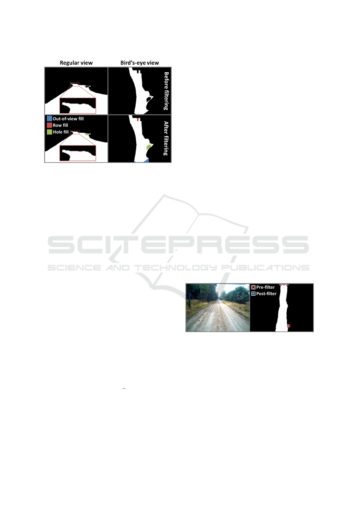
Figure 3: Mask ﬁltering impact example. The impact of

row-gap ﬁlling is enhanced and highlighted in red at the top

of the road, out-of-view ﬁlling is shown in blue and hole

ﬁlling in green.

able starting point from which the path planning is

commencing. Note that this point can be slightly in

front of the vehicle depending on camera tilt, because

the camera is at a certain height above the ground

and has limited vertical ﬁeld of view. Hence, the bot-

tom row of pixels in the original image, which corre-

sponds to the bottom row of pixels in the BEV image,

is aligned with the line where the vertical ﬁeld of view

of the camera intersects with the ground plane. In our

test setup, the tilt of the PTZ camera is set such that

this point is approximately four meters in front of the

vehicle.

Detection of End Point(s). In order to ﬁnd all viable

road centerlines, end points should be located on all

branching roads in the image. For example, an inter-

section generally results in three viable road center-

lines. Potential endpoints are detected by applying a

Breadth First Search (BFS) on the BEV road mask.

This search returns an image where every pixel has

a value representing the distance to the start point.

End points are then estimated by ﬁnding local max-

ima in the resulting image. To prevent a large number

of spurious maxima at rough edges of the mask, we

consider a local maximum only if it is the maximum

value within a certain window size, instead of merely

comparing to adjacent pixels.

Improving the BFS is one way to achieve more

reliable endpoints. We modify the 8-way BFS so

that moving diagonally costs

√

2 movement instead

of unity. This improves the detection of end points

for side roads or roads with strong curves, as the ap-

proximated distance is closer to a Euclidean distance.

End point(s) Filtering. Using the above algorithm,

results in several incorrect end points. The majority

of these incorrect end points are caused by two as-

pects. First, due to the way that endpoints are de-

tected, namely using BFS, the end points may not end

up in the middle of the road, but instead at the cor-

ners of the road mask, because they are slightly fur-

ther away. This only causes the last part of the path

to be incorrect, but this issue is still worth addressing.

To alleviate this problem, we search for end points at

the top row of road mask pixels and merge (in case

of two end points connected by only white pixels) or

move them (in case of a single end point) to the cen-

ter of this row of pixels. An example is shown at the

top of Fig. 4. The issue is now resolved for straight

roads, but end points for curved roads may also be

moved incorrectly. To prevent moving end points of

curved roads, end points are only moved if their hori-

zontal positions are within the width of the road at the

bottom of the BEV, plus a small margin. The second

cause of incorrect end points is shape deviations in the

road mask, which primarily appear when the road is

not clearly separable from the roadside. This happens

most often close to the vehicle, where the high reso-

lution allows for example small clumps of grass to be

detected as “not road”, as in the bottom right of Fig. 4.

In practice, because this issue only appears close to

the vehicle, we simply ﬁlter out road end points that

appear too close to the vehicle. In case there really is

a road fork this close to the vehicle, the camera should

have been tracking it earlier, and would have rotated

its orientation such that the fork would no longer be

at the side of the view. Hence, we can conclude that

this road fork is not the desired path anyway.

Figure 4: Example of end point ﬁltering which shows both

centering end points at road endings and ﬁltering out nearby

end points.

Path Finding. To ﬁnd a path through the center of the

road from the start point to all end points, a distance

transform is applied to the BEV road mask, inverted

and then used as the cost for an A* path-ﬁnding al-

gorithm. The low cost far away from non-road pixels

causes the A* algorithm to ﬁnd a path as far away as

possible from these non-road pixels, which approxi-

mates the center of the road.

When taking the regular distance transform of an

image, at every pixel, the distance to the nearest zero

pixel is returned. Local high values in the distance

VISAPP 2023 - 18th International Conference on Computer Vision Theory and Applications

558

transform are a good approximation of the center of

the road, as long as the road touches both the top and

bottom of the BEV image. In cases where distant road

is occluded, for example due to a height difference,

the road mask in the BEV will end partway in the im-

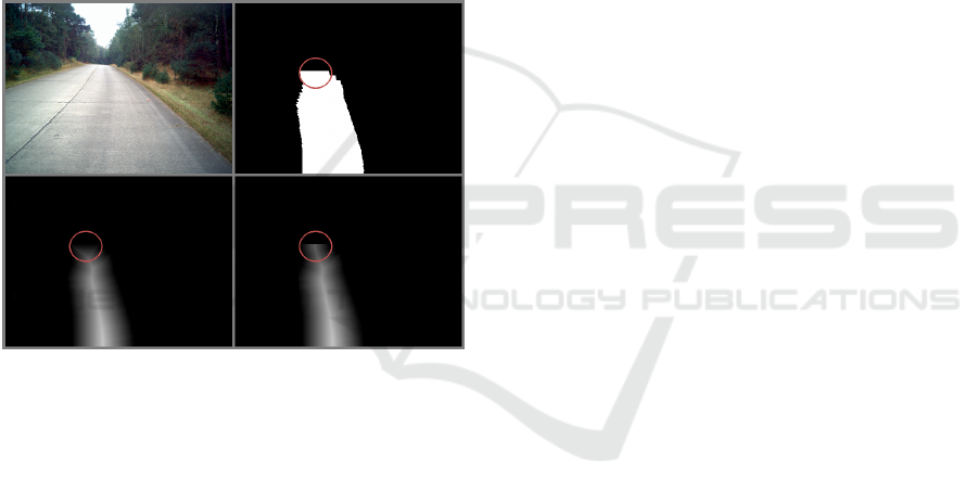
age. An example of this is shown in Fig. 5. As can be

observed at the bottom left of the Figure, this causes

the high values in the distance transform to no longer

align with the center of the road. To remedy this,

the BEV mask is temporarily modiﬁed by changing

the pixel values of the rows above the top-most road-

mask pixel to white, after which the distance trans-

form is applied. The rows of changed pixels are then

set back to black in the distance transform, resulting

in the bottom-right image of Fig. 5. A similar process

can be applied for cases where the road pixels do not

start at the bottom-most row of the BEV, although this

case is uncommon.

Figure 5: Modiﬁed distance transform example. The local

maxima of the distance transform now more clearly follow

the center of the road, all the way until the end of the road

mask.

4 EXPERIMENTAL RESULTS

The resulting path-ﬁnding system performs well on

our private datasets. In the following sections, the

road segmentation and path-ﬁnding results are dis-

cussed separately. For road segmentation, we primar-

ily investigate the impact of training with different

datasets.

4.1 Impact of Datasets on Performance

The selection of datasets that are used to train the road

segmentation model has a large impact on the perfor-

mance. To evaluate the impact of each dataset on un-

structured road segmentation performance, we ﬁne-

tune the Mseg-pretrained HRNet-W48 for 10 epochs

on each individual dataset and test the road segmen-

tation performance on our two validation datasets

in the Netherlands (NL-val) and Austria (AT-val).

The road IoU of the WildDash validation set (WD-

val) is reported to verify that the model is not over-

trained on only unstructured or unpaved roads, but

the performance on this dataset is not leading for

our application. The results of ﬁne-tuning on indi-

vidual datasets are listed in the middle block of Ta-

ble 1. “Mseg HRNet-W48” refers to the model spre-

trained by (Grigorescu et al., 2020) on ADE20K,

BDD100K, Cityscapes, COCO-Panoptic, IDD, Map-

illary Vistas and SUNRGBD. “Public” refers to all

public datasets that we found to be potentially use-

ful for unstructured road segmentation: BDD100K,

Cityscapes, IDD, Mapillary Vistas, Freiburg Forest,

RUGD and YCOR. A Cityscapes-pretrained PSPNet-

50 (Zhao et al., 2017) is included as a baseline.

From the bottom half of Table 1, it could be con-

cluded that some datasets are not worth combining,

as they cause rather poor IoU scores on our own

recorded datasets when applied independently. The

most extreme case of this is the RUGD dataset, which

is likely due to the extremely low viewpoint, driving

mostly besides the road instead of on it, and having a

limited variety of road types. The top half of Table 1

shows the results of combining multiple datasets to

further improve the performance. It shows that re-

moving the lower-performing RUGD data can indeed

improve accuracy in some cases, but the impact is mi-

nor enough such that simply combining all possible

relevant datasets seems to be a reasonable guideline

in general.

4.2 Path-Finding Qualitative Results

The path planning is difﬁcult to evaluate quantita-

tively without extensive manual labeling effort, there-

fore we focus on reporting some failure cases that

persist even after using our best segmentation model

(trained on Public+NL) and applying all the path-

planning improvements described in Sections 3.2.1

and 3.2.2. The NL-val dataset shows worse path-

ﬁnding failures than the AT-val dataset, hence the ex-

amples displayed here are all from NL-val.

Fig. 6 shows four different path-ﬁnding failure

cases, with blue borders indicating the detected road

and the red lines the estimated centerline(s). In (a),

a noisy offshoot from the segmentation is sufﬁciently

far away, such that after the BEV transformation it

becomes sufﬁciently large to be recognized as a side

road. This is hard to repair afterwards, hence it would

likely require a better segmentation, and thus a better

trained network, to prevent this. In (b), a tire-track

Robust Path Planning in the Wild for Automatic Look-Ahead Camera Control

559

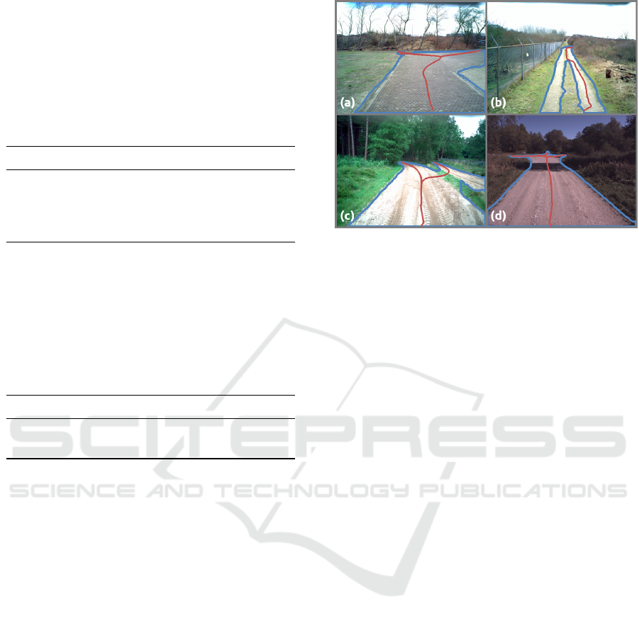
Table 1: Results of ﬁne-tuning the HRNet-W48 network

on several different (combinations of) datasets, where bold

scores are highest and italic are second-highest. Top block

of the table has been trained on combinations of datasets,

middle block on single datasets and bottom block are pre-

trained networks from other authors. Each block is sorted

by the mean IoU. *(Note: only road segmentation is eval-

uated, not any other classes, hence these WildDash scores

cannot directly be compared to other works that evaluate on

it).

Train Dataset NL-val AT-val WD-val* Mean

Public+NL 0.928 0.964 0.844 0.912

Public+NL-RUGD 0.927 0.961 0.840 0.909

Public-RUGD 0.907 0.944 0.849 0.900

Public 0.814 0.943 0.818 0.858

YCOR 0.927 0.941 0.784 0.884

IDD 0.875 0.911 0.878 0.888

NL 0.918 0.945 0.593 0.819

Cityscapes 0.886 0.875 0.878 0.880

Mapillary Vistas 0.551 0.805 0.828 0.728

Freiburg Forest 0.652 0.773 0.496 0.640

Rellis3D 0.733 0.733 0.515 0.660

BDD 0.256 0.687 0.829 0.591

RUGD 0.138 0.030 0.371 0.179

Pretrained baselines

Mseg HRNet-W48 0.395 0.880 0.809 0.695

PSPNet-50 0.609 0.378 0.538 0.508

road is detected as two separate roads. This failure

case is common, because all public datasets with tire-

track roads also annotate it as separate tracks. Hence,

manual relabeling of the public datasets is likely the

easiest solution, but time-consuming. In (c), two par-

allel roads separated by some grass are partially de-

tected as a single road. This is the opposite of the

problem in (b): it looks similar to a tire track with

grass in the middle, and our private dataset has tire

tracks annotated as a single blob, causing this edge-

case error. This error only happens in this speciﬁc

frame and nowhere else in the dataset, hence it is

probably not a big issue. In (d), a 4-way crossing re-

sults in 5 detected paths. This is rather common when

the crossing is still far away, because the shape is not

yet well-deﬁned. This problem solves itself once the

vehicle more closely approaches the crossing, thus it

is not a real problem in practice.

Overall, the failure cases are deemed acceptable

for the application of camera control, but applica-

tion of the proposed algorithm for autonomous driv-

ing may require additional robustness improvements,

such as temporal ﬁltering.

Figure 6: Path-ﬁnding failure cases in the NL-val dataset.

Road segmentations are outlined in blue, estimated center-

lines in red. (a) Noisy segmentation offshoot, (b) sepa-

rated tire-track road, (c) merged close-together roads, (d)

too many paths at intersection (spurious tiny path at top

left).

5 DISCUSSION

Although the path-planning system works well on our

test cases, it also has several limitations. First, while

many road types are now present in the combined

dataset, there are still edge cases that are not captured.

For example, the unpaved road datasets do not contain

many images in the dark or with rainy weather, hence

performance in those situations is likely to remain

limited, as can be partly observed from the WildDash

dataset performance.

Second, even though the ﬁnal performance on our

test set is considered good, the performance with only

the seven public datasets, thus without the NL images,

is moderate at the NL-val set, which shows that gener-

alizing to new road types still remains difﬁcult. Over-

all, there is still a lack of good public datasets, even

small ones, that contain all possible road types.

Third, the path-planning algorithm currently does

not take other road users into account. While this is

actually beneﬁcial to our speciﬁc use case of camera

control, it is detrimental when applying this algorithm

for autonomous driving. Thus, when trying to use

our work for autonomous driving, the most valuable

part is the robust road segmentation and not the path-

ﬁnding algorithm.

6 CONCLUSION

In this paper we have proposed a robust path-planning

system for any type of road, with a focus on un-

VISAPP 2023 - 18th International Conference on Computer Vision Theory and Applications

560

paved roads. There are two main contributions. First,

we have combined seven public driving and robotics

datasets, which together contain a large variety of

road types, and trained a HRNet-W48 network on this

data to achieve robust road segmentation. Second,

we have developed a path-ﬁnding algorithm and im-

proved its robustness to incorrect road segmentation

in several ways, allowing for automated control of a

vehicle-mounted PTZ camera, which can handle road

crossings and forks.

Our experimental results have shown that individ-

ual driving datasets contain insufﬁcient variety to al-

low training of a robust road segmentation system

for all road types. Combining seven different pub-

lic datasets and adding just a small number of semi-

automatically labeled images greatly improves the

performance to the point that all roads in the test

dataset can be accurately segmented. Although this

paper is primarily concerned with camera control, the

robust road segmentation for a broad class of roads

can also be of interest for work in autonomous driv-

ing.

Overall, we conclude that robust path planning on

any type of road is feasible, but will still require com-

parable extensive datasets that autonomous driving re-

search has generated for urban environments over the

past few years. Until then, combining many existing

datasets is a good alternative for generalization.

REFERENCES

Cordts, M., Omran, M., Ramos, S., Rehfeld, T., Enzweiler,

M., Benenson, R., Franke, U., Roth, S., and Schiele,

B. (2016). The Cityscapes Dataset for Semantic Urban

Scene Understanding. In CVPR 2016.

Giusti, A., Guzzi, J., Ciresan, D. C., He, F. L., Rodriguez,

J. P., Fontana, F., Faessler, M., Forster, C., Schmid-

huber, J., Caro, G. D., Scaramuzza, D., and Gam-

bardella, L. M. (2016). A Machine Learning Ap-

proach to Visual Perception of Forest Trails for Mo-

bile Robots. IEEE Robotics and Automation Letters,

1(2):661–667.

Gonz

alez, D., P

erez, J., Milan

es, V., and Nashashibi, F.

(2016). A Review of Motion Planning Techniques for

Automated Vehicles. IEEE Transactions on Intelli-

gent Transportation Systems, 17(4):1135–1145.

Grigorescu, S., Trasnea, B., Cocias, T., and Macesanu,

G. (2020). A survey of deep learning techniques

for autonomous driving. Journal of Field Robotics,

37(3):362–386.

Jiang, P., Osteen, P., Wigness, M., and Saripalli, S. (2020).

RELLIS-3D dataset: Data, benchmarks and analysis.

arXiv 2011.12954v2.

Maturana, D., Chou, P.-W., Uenoyama, M., and Scherer,

S. (2018). Real-Time Semantic Mapping for Au-

tonomous Off-Road Navigation. In Springer Proceed-

ings in Advanced Robotics, pages 335–350.

Nakagomi, H., Fuse, Y., Nagata, Y., Hosaka, H., Miyamoto,

H., Yokozuka, M., Kamimura, A., Watanabe, H., Tan-

zawa, T., and Kotani, S. (2021). Forest road sur-

face detection using LiDAR-SLAM and U-Net. 2021

IEEE/SICE International Symposium on System Inte-

gration, pages 727–732.

Neuhold, G., Ollmann, T., Bulo, S. R., and Kontschieder,

P. (2017). The Mapillary Vistas Dataset for Semantic

Understanding of Street Scenes. In ICCV 2017.

Paden, B.,

ap, M., Yong, S. Z., Yershov, D., and Fraz-

zoli, E. (2016). A survey of motion planning and con-

trol techniques for self-driving urban vehicles. IEEE

Transactions on Intelligent Vehicles, 1(1):33–55.

Qureshi, A. H., Simeonov, A., Bency, M. J., and Yip, M. C.

(2019). Motion planning networks. In Proceedings -

IEEE International Conference on Robotics and Au-

tomation, volume 2019-May, pages 2118–2124.

Ronneberger, O., Fischer, P., and Brox, T. (2015). U-Net

: Convolutional Networks for Biomedical. In Med-

ical Image Computing and Computer-Assisted Inter-

vention (MICCAI), pages 234–241.

Shelhamer, E., Long, J., and Darrell, T. (2016). Fully con-

volutional networks for semantic segmentation. IEEE

Transactions on Pattern Analysis and Machine Intel-

ligence, 39(4):640–651.

Sun, K., Zhao, Y., Jiang, B., Cheng, T., Xiao, B., Liu, D.,

Mu, Y., Wang, X., Liu, W., and Wang, J. (2019). High-

resolution representations for labeling pixels and re-

gions. arXiv 1904.04514v1.

Valada, A., Oliveira, G. L., Brox, T., and Burgard, W.

(2016). Deep Multispectral Semantic Scene Under-

standing of Forested Environments Using Multimodal

Fusion. In International Symposium on Experimental

Robotics (ISER).

Varma, G., Subramanian, A., Nboodiri, A., and Chandraker,

M. (2019). IDD : A Dataset for Exploring Problems of

Autonomous Navigation in Unconstrained Environ-

ments. In IEEE Winter Conference on Applications

of Computer Vision (WACV).

Wigness, M., Eum, S., Rogers, J. G., Han, D., and Kwon,

H. (2019). A RUGD Dataset for Autonomous Navi-

gation and Visual Perception in Unstructured Outdoor

Environments. IEEE International Conference on In-

telligent Robots and Systems, pages 5000–5007.

Yadav, S., Patra, S., Arora, C., and Banerjee, S. (2017).

Deep CNN with Color Lines Model for Unmarked

Road Segmentation. In IEEE International Confer-

ence on Image Processing (ICIP), pages 585–589.

Yu, F., Chen, H., Wang, X., Xian, W., Chen, Y., Liu, F.,

Madhavan, V., and Darrell, T. (2020). BDD100K: A

Diverse Driving Dataset for Heterogeneous Multitask

Learning. In CVPR 2020, pages 2633–2642.

Zendel, O., Honauer, K., Murschitz, M., Steininger, D.,

and Dom

ınguez, G. F. (2018). WildDash - Creating

Hazard-Aware Benchmarks. In Proceedings of ECCV,

pages 407–421.

Zhao, H., Shi, J., Qi, X., Wang, X., and Jia, J. (2017). Pyra-

mid Scene Parsing Network. In CVPR.

Robust Path Planning in the Wild for Automatic Look-Ahead Camera Control

561