Particle Tracking with Neighbourhood Similarities: A New Method for
Super Resolution Ultrasound Imaging
Andrew Mobberley
1
, Georgios Papageorgiou
1
, Mairead Butler
1
, Evangelos D. Kanoulas
2
,
Julian Keanie
3
, Daniel Good
3
, Kevin Gallagher
3
, Alan McNeil
3
, Vassilis Sboros
1
and Weiping Lu
1
1
Institute of Biological Chemistry, Biophysics and Bioengineering, Heriot Watt University, Edinburgh, U.K.
2
Janssen Pharmaceuticals R&D, High Wycombe, U.K.
3
Western General Hospital, Edinburgh, U.K.
Keywords:
Super Resolution Ultrasound Imaging, Particle Tracking, Microbubbles.
Abstract:
Single particle tracking (SPT) is a method for the observation of the motion of individual particles within
a medium. It is broadly used to quantify the dynamics of particle flow, such as molecules/proteins in life
sciences. In this paper, we will improve the performance of SPT by considering the local neighbourhood
dynamical and structural information of a particle when it is tracked in a medium through consecutive frames,
referred to as particle tracking with neighbourhood similarities (PTNS). This method is applied to track mi-
crobubbles in contrast enhanced ultrasound. We will test the method on synthetic data for method validation
before applying to animal and human prostate data. We show that PTNS can make a significant improvement
in the tracking performance in synthetic data, and in animal data it was able to accurately produce complex
structures. In human prostate data, we find that by varying the control parameters we can inspect different
behaviours of the tracks and from that understand the characteristics of the blood vessels they travel along.
1 INTRODUCTION
Contrast-enhanced ultrasound (CEUS) is an imaging
modality used in hospitals to depict the circulation
of organs within the body (Xu, 2009). Microbub-
bles (MBs) that act as contrast agents are injected
into the patient intravenously before the imaging takes
place to enhance the ultrasound image (Sboros, 2008).
While CEUS has a higher image contrast compared
to conventional ultrasound, its resolution is still lim-
ited by the fundamental wave diffraction limit, which
is around 1mm for ultrasound waves (Couture et al.,
2018). Such resolution limitations also occur in other
imaging devices, such as optical microscopy due to
light diffraction.
Several methods have recently been developed
in super resolution that can surpass the fundamental
diffraction limit, referred to as super resolution imag-
ing. Photoactivated localisation microscopy (PALM)
is one such technique that can localise fluorophores
in optical images with spatial accuracy much better
than the diffraction limit, thus achieving super resolu-
tion optical imaging many times below the diffraction
limit (Betzig et al., 2006; Hess et al., 2006). This
work in optical microscopy has inspired a similar ap-
proach in ultrasound by localising MBs in CEUS data
(Couture et al., 2018; Errico et al., 2015). Super reso-
lution ultrasound imaging (SRUI) is considered a ma-
jor development in the field since the discovery of ul-
trasound imaging.
The key to achieving SRUI is particle tracking,
which comprises three steps: particle detection, lo-
calisation and linking. Detection of MBs can be
achieved either by using particle probability images
(Yang et al., 2012) or by using comparisons to a ref-
erence MB signal (Brown et al., 2019). Since they are
much smaller than the imaging wavelength, they need
to be localised, for example, by identifying the cen-
troids of the MB signals (Couture et al., 2018; Errico
et al., 2015; Yang et al., 2012; Brown et al., 2019).
The motion of these MBs is then approximated by
linking the localised positions between consecutive
frames.
Many linking strategies have been developed for
particle tracking. However, they have all been devel-
oped under the common rationale that the MBs with
the shortest distance between subsequent frames are
most likely to be linked. The most popular of these
Mobberley, A., Papageorgiou, G., Butler, M., Kanoulas, E., Keanie, J., Good, D., Gallagher, K., McNeil, A., Sboros, V. and Lu, W.
Particle Tracking with Neighbourhood Similarities: A New Method for Super Resolution Ultrasound Imaging.
DOI: 10.5220/0011613900003414
In Proceedings of the 16th International Joint Conference on Biomedical Engineering Systems and Technologies (BIOSTEC 2023) - Volume 2: BIOIMAGING, pages 29-40
ISBN: 978-989-758-631-6; ISSN: 2184-4305
Copyright
c
 2023 by SCITEPRESS – Science and Technology Publications, Lda. Under CC license (CC BY-NC-ND 4.0)
29

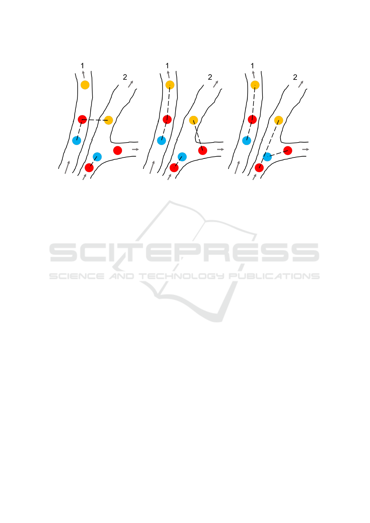
(a) (b) (c)
Figure 1: Visualisation of different linking strategies that can be employed for MB tracking. The blue, red and yellow circles
represent MBs in the first, second and third frame respectively. The dashed lines represent the links. 1a shows the nearest
neighbour method. 1b shows the motion model method. 1c shows the ground truth links.
methods is the nearest neighbour method (NN) (Maz-
zaferri et al., 2014; Godinez et al., 2009). An illus-
tration of how NN links MBs is depicted in Figure
1a. According to this method, MBs in one frame
are linked to the nearest MB in the next frame, re-
gardless of flow direction or whether the MBs share
the same vessel. For sparse MB fields, this method
works well (Kanoulas et al., 2019), capable of con-
structing the vessel networks using MB tracks, even
in low signal-to-noise ratio environments. However,
as MB density increases, the number of errors pro-
duced by NN also increases (Opacic et al., 2018). To
improve the linking accuracy of NN, motion mod-
els are added by imposing certain motion restrictions
between frames, which is visualised in Figure 1b.
These motion models can be simple, such as linear
flows(Opacic et al., 2018; Tang et al., 2020), or more
complex ones, such as the interactive multiple model
(IMM)(Genovesio et al., 2006) which accommodate
many different types of particle motion and also in-
corporate the particle size and intensity (Yang et al.,
2012). Motion model linking strategies typically per-
form better than those which use the nearest neigh-
bour method (Chenouard et al., 2014), and have pro-
duced good results when applied to CEUS images
(Opacic et al., 2018; Tang et al., 2020; Kanoulas,
2020).
The main objective of SRUI is to visualise the
structure and dynamics of vessels at resolutions down
to the near-microscopic scale (Opacic et al., 2018;
Lin et al., 2016). To achieve this objective, the link-
ing of MBs between different blood vessels should
be avoided. Incorrect links affect the quality of the
super resolution vascular reconstruction, causing the
images to appear noisy. Moreover, MB linking should
strictly follow the vessel structure even when the ves-
sels bend and the frame frequency is limited, as is the
case for clinical scanners; using a straight-line link in
curved vessels reduces the spatial resolution. Addi-
tionally, even with an appropriate motion model for
MB linking, the first link in a track remains prob-
lematic as there is no velocity information available.
NN in this situation could not only result in a wrong
track for itself but also affect neighbouring tracks. Fi-
nally, the point spread function of ultrasound imaging
varies spatially (Kanoulas et al., 2019), meaning that
the topological features of MBs are not robust enough
to be used in the IMM filter. These issues can only be
addressed with further improvements of the linking
approaches available in the literature.
In this paper, we propose a new method which
we call Particle Tracking with Neighbourhood Sim-
ilarities (PTNS) to tackle the aforementioned issues.
This method is based on two observations in our re-
cent study of ultrasound imaging. First, since MBs
are confined in vessels, MB linking should be avoided
when there is not sufficient and continuous MB den-
sity along its path. Second, MBs around a local neigh-
bourhood are likely to belong to the same vessel and
so should have similar directions and speeds. These
observations are analogous to how vehicles travel on
a road.
This paper is arranged as follows. In Section 2.1,
we provide an overview of PTNS. Sections 2.2, 2.3
BIOIMAGING 2023 - 10th International Conference on Bioimaging
30

and 2.4 describes the method in more detail. In Sec-
tion 3, we describe the experiments used for test-
ing PTNS, and finally we conclude by discussing our
findings.
2 MATERIALS AND METHODS
2.1 Particle Tracking with
Neighbourhood Similarities
To incorporate the above mentioned observations into
PTNS, we first measure the MB density to define
criteria that each link must meet in order to be ac-
cepted. These criteria are called density assisted link-
ing, which will prevent links from being made be-
tween adjacent vessels. Second, we use the collective
speed and direction information within a local neigh-
bourhood to guide the linking. This is called velocity
assisted linking, which will assist the first link in a
track.
PTNS is implemented by running the particle
tracking process twice, referred to as a two run pro-
cess, as depicted in Figure 2. In the first run (R1),
shown in the left dashed box, MBs are detected using
the particle probability (Yang et al., 2012). Linking is
performed using the NN and motion model methods,
where each potential link is assigned a cost within a
matrix. The cost is based on the distance between
MBs in adjacent frames. This cost matrix is then
minimised to find the appropriate link for each MB
(Yang et al., 2012). Density assisted linking is ap-
plied here to refine the tracks. In the second run (R2),
shown in the right dashed box, we apply velocity as-
sisted linking using the velocity information gathered
in R1. This will further refine the linking after den-
sity assisted linking has been applied, particularly for
the first link in a track. Moreover, we introduce a
new maximum density seeking method to re-evaluate
the links that were rejected by density assisted link-
ing to find whether an alternate, bending link exists
(instead of a straight line link). These three new link-
ing strategies, i.e. density assisted linking, velocity
assisted linking and maximum density seeking, will
be described in more detail in Sections 2.2, 2.3, 2.4
respectively.
2.2 Microbubble Density Assisted
Linking
Our linking strategy involves minimising the cost ma-
trix C. For the MBs identified in frame t, m
m
m
i
where
i = 1, ...,M are the number of MBs, we predict their
positions in frame t +1, m
m
m
′
i
, by using the motion mod-
els. These are then compared to the MBs identified in
frame t + 1, n
n
n
j
where j = 1, ..., N are the number of
MBs in the next frame. The cost matrix is constructed
as
C =





d(m
m
m
′
1
− n
n
n
1
)
2
d(m
m
m
′
1
− n
n
n
2
)
2
··· d(m
m
m
′
1
− n
n
n
N
)
2
d(m
m
m
′
2
− n
n
n
1
)
2
d(m
m
m
′
2
− n
n
n
2
)
2
··· d(m
m
m
′
2
− n
n
n
N
)
2
.
.
.
.
.
.
.
.
.
.
.
.
d(m
m
m
′
M
− n
n
n
1
)
2
d(m
m
m
′
M
− n
n
n
2
)
2
··· d(m
m
m
′
M
− n
n
n
N
)
2





,
(1)
where
d(m
m
m
′
i
− n
n
n
j
)
2
= (m
′
i,x
− n
j,x
)
2
+ (m
′
i,y
− n
j,y
)
2
, (2)
is the distance and m
m
m
′
i
= (m
′
i,x
, m
′
i,y
) and n
n
n
j
=
(n
j,x
, n
j,y
) are the coordinates of the MBs. Links are
made by minimising each row of equation 1 and opti-
mised so that each MB is linked to and by one MB in
two consecutive frames.
As discussed in Section 1, density assisted linking
is a key restriction to prevent links from being made
between different vessels. For an image sequence
under investigation, the MB density, ρ(x, y), in pixel
(x, y) is defined as the number of MBs localised in this
pixel for all image frames. Since MBs travel within
vessels, correct links between m
m
m
i
and n
n
n
j
should satisfy
the following minimum MB density criteria, which in
turn update C. The first condition is,
C(i, j) =

d(m
m
m
′
i
− n
n
n
j
)
2
if
¯
ρ > c
ρ
(ρ(m
m
m
i
) + ρ(n
n
n
j
))
∞ otherwise
,
(3)
where
¯
ρ is the average MB density over all the pixels
along the straight-line path between m
m
m
i
and n
n
n
j
. Equa-
tion 3 ensures that there is sufficient MB density along
the trajectory between the start and end pixels, which
will prevent links from being made between neigh-
bouring vessels (Kanoulas, 2020). The hyperparame-
ter c
ρ
, defined as a percentage of (ρ(m
m
m
i
) + ρ(n
n
n
j
)), is
a control parameter for accepting or rejecting a link.
The second density assisted linking condition is,
C(i, j) =

d(m
m
m
′
i
− n
n
n
j
)
2
if σ
ρ
< c
σ
¯
ρ
∞ otherwise
, (4)
where σ
ρ
is the standard deviation of the MB density
over all the pixels along the straight-line path between
m
m
m
i
and n
n
n
j
and c
σ
is a hyperparameter. Equation 4 en-
sures that the MB density does not fluctuate signifi-
cantly along the path between m
m
m
i
and n
n
n
j
. The hyper-
parameter c
σ
controls how large the fluctuation of the
MB density can be before the link is rejected.
In summary, the density criteria given in equations
3 and 4 require that along the trajectory of a track,
there must be a sufficient number and a smooth dis-
tribution of MBs, thereby avoiding jumps of MBs be-
tween vessels and improving the vessel reconstruc-
tion.
Particle Tracking with Neighbourhood Similarities: A New Method for Super Resolution Ultrasound Imaging
31

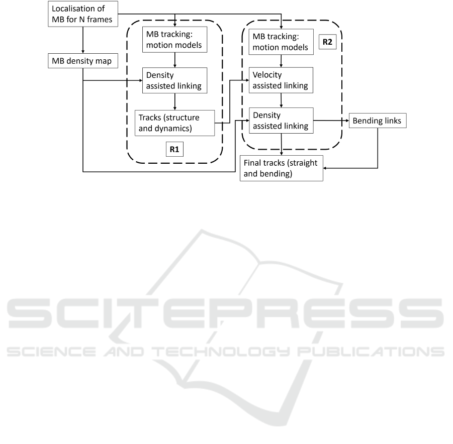
Figure 2: Flow chart of PTNS applied to CEUS data. The first run is shown in the dashed box labeled R1 and the second run
is shown in the dashed box labeled R2.
2.3 Velocity Assisted Linking
As described earlier, we use motion models to better
predict how MBs move within vessels, but these re-
quire velocity information from previous links. For
the first link in a track, there is no velocity informa-
tion and so the link can only be made using NN. We
have developed a method to guide the links based on
speed and direction information provided by the local
neighbourhood: velocity assisted linking.
We implement this concept in the second run of
PTNS (R2), which is depicted by the right dashed
box in Figure 2. On the completion of the first run
(R1), we can use all the MB tracks to generate their
speed and direction maps, v(x, y) and θ(x, y), which
are the average speed and direction of the tracks pass-
ing through pixel (x, y) respectively. We can further
calculate the standard deviation of the speed and di-
rection of these tracks passing through each pixel,
σ
v
(x, y) and σ
θ
(x, y) respectively. These four mea-
surements will then be incorporated into the linking
in R2.
When a MB travels along a vessel, its speed
and direction vary between neighbouring frames but
should be within a certain continuity range. Here, we
introduce two velocity assistance criteria, fixed and
variable continuities respectively, suitable to different
data sets under investigation. Which criterion is best
applicable depends on the results obtained in R1. The
fixed continuity criterion is best applicable when all
the tracks in the entire image have fairly good conti-
nuity in both speed and direction, and their variations
both locally and globally are small and well defined.
In this case, the cost matrix C can be updated as
C(i, j) =





d(m
m
m
′
i
− n
n
n
j
)
2
if β
1
v(m
m
m
i
) < v < β
2
v(m
m
m
i
)
and
θ(m
m
m
i
) − Θ < θ < θ(m
m
m
i
) + Θ
∞ otherwise
,
(5)
where v and θ are the speed and direction of the link
between MBs m
m
m
i
and n
n
n
j
, and m
m
m
i
= (m
i,x
, m
i,y
) are the
pixel coordinates of MB m
m
m
i
in frame t. The coeffi-
cients β
1
and β
2
are the scaling parameters giving the
fixed lower and upper boundaries of the speed respec-
tively, β
1
< 1 and β
2
> 1. The angle Θ defines the
fixed angle variation allowed around θ(m
m
m
i
). All three
parameters can be estimated from R1.
The second criterion applies when the speed and
direction continuity is not consistent, varying signifi-
cantly across the image. In this case, the variable con-
tinuity criterion is more appropriate and C is updated
as
C(i, j) =













d(m
m
m
′
i
− n
n
n
j
)
2
if v(m
m
m
i
) − γσ
v
m
m
m
i
) < v <
v(m
m
m
i
) + γσ
v
(m
m
m
i
)
and
θ(m
m
m
i
) − γσ
θ
(m
m
m
i
) < θ <
θ(m
m
m
i
) + γσ
θ
(m
m
m
i
)
∞ otherwise
,
(6)
where γ is a parameter that controls how narrow the
continuity range is. A lower value of γ results in
a more restrictive continuity range. As observed in
equation 6, the restriction varies from pixel to pixel
depending on the standard deviation of the speed and
direction in that pixel.
The above two criteria given in equations 5 and 6
each have advantages and disadvantages and will be
applicable to some data sets more than others. The
BIOIMAGING 2023 - 10th International Conference on Bioimaging
32

(a) (b)
Figure 3: The potential links that can be made using R1 and R2. A MB in frame t is shown as a red circle, and the candidate
MBs it could be linked to in frame t + 1 are shown as orange circles. The correct MB is shown with a green border. The gray
arrows show the direction of the blood flow, and the dashed black lines show the potential links which can be made from the
starting MB. There are more possible potential links in R1, 3a, than there are in R2, 3b. How velocity assisted linking restricts
the potential links based on the speed and direction continuity is shown by the gray dashed lines in 3b.
former is homogeneous across the image but contains
three free parameters to be adjusted, whereas the lat-
ter has a single parameter to set. As discussed earlier,
which criterion is best suited with what parameter val-
ues is determined by the first run, which will be fur-
ther discussed in the Section 3 when a specific data
set is tested. Since the first link of any track can apply
the speed and direction information in R2 from the
other tracks in its neighbourhood, already available
from R1, this link is no longer made using only the
nearest neighbour method as in R1. Along with the
motion models, all links produced by PTNS use the
velocity information from the local neighbourhood,
and thus all the tracks have a certain degree of con-
tinuity in both speed and direction, set by the control
parameters. This process is visualised in Figure 3.
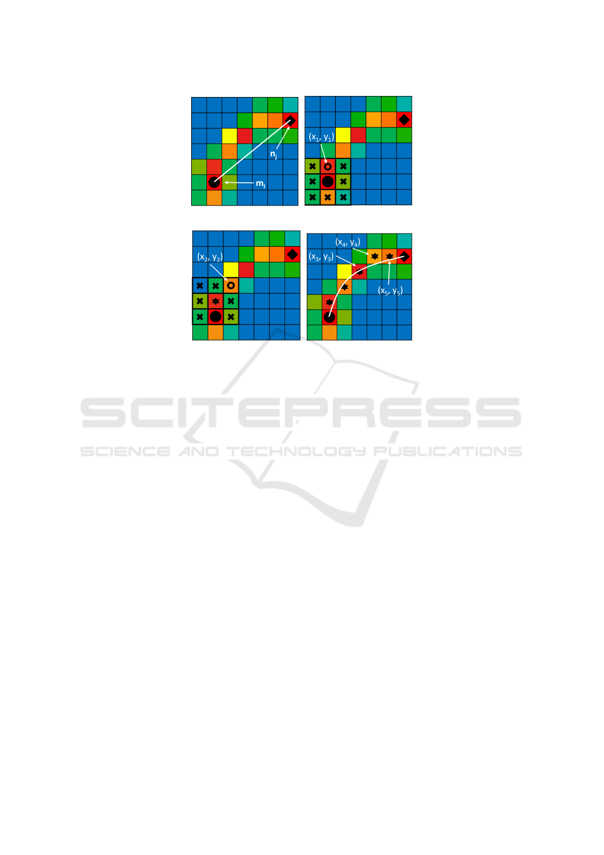
2.4 Maximum Density Seeking
When equations 3 and 4 are applied, a link previously
accepted by the motion models may be accepted or re-
jected. If a link is accepted, then it can be used to form
part of a track. If a link is rejected, it could genuinely
be wrong, or it may be correct but the straight line
path may be wrong as the vessel bends significantly
at this location. For the latter case, an alternate, non-
straight trajectory is more realistic. We propose a new
maximum density seeking method to recover such a
path after the straight-line link has been rejected.
The method finds a path with maximum MB den-
sity between two consecutive frames, which is re-
ferred to as bending links in Figure 2.
As shown in Figure 4a, after the straight-line link
from m
m
m
i
to n
n
n
j
is rejected by the path density criteria, a
pixel among the 8 neighbours of m
m
m
i
, which has a MB
density above a certain threshold and has the shortest
distance to n
n
n
j
compared to the other pixels, is chosen
as the next stage in the linking process. This pixel is
labeled as (x
1
, y
1
) in Figure 4b. This process is re-
peated by sliding the neighbourhood window from m
m
m
i
to (x
1
, y
1
) as shown in Figure 4c. Continuing the pro-
cess leads to successive link points (x
3
, y
3
), (x
4
, y
4
),
..., (x
N
, y
N
), until n
n
n
j
, forming the bending link from
m
m
m
i
to n
n
n
j
shown in Figure 4d. If (x
N
, y
N
) cannot reach
n
n
n
j
, the process fails and no alternative path is possi-
ble.
3 RESULTS
To test the new linking strategies, we will apply PTNS
to three different data sets: synthetic, animal and hu-
man prostate CEUS images. These data sets will al-
low us to quantitatively and qualitatively assess the
performance of PTNS under various different condi-
tions, some of which have distinct and known char-
acteristics that can be compared to the structural and
dynamical features recovered by PTNS.
3.1 Synthetic Data Test
A synthetic flow model is first generated to simulate
blood flow in a vascular network. Point-like particles
are then injected into the network, moving along the
Particle Tracking with Neighbourhood Similarities: A New Method for Super Resolution Ultrasound Imaging
33

(a) (b)
(c) (d)
Figure 4: The steps of the maximum density method. Pixels with high MB density are shown in red, orange and yellow. Pixels
with low MB density are shown in green, and pixels with no MBs detected are shown in blue. The black circle and diamond
show the starting and ending pixel, m
m
m
i
and n
n
n
j
, respectively. 4a: the straight-line link between m
m
m
i
and n
n
n
j
is rejected because it
violates the density criteria. 4b: the neighbourhood around m
m
m
i
is inspected and the nearest pixel to n
n
n
j
which is above the pixel
threshold is labeled (x
1
, y
1
). 4c: the process is repeated by inspecting the neighbourhood around (x
1
, y
1
) to find (x
2
, y
2
). 4d:
The process continues, finding (x
3
, y
3
), (x
4
, y
4
) and (x
5
, y
5
). The bending link is then fitted from m
m
m
i
to n
n
n
j
through the pixels
of highest density (x
1
, y
1
) to (x
5
, y
5
).
flow. These particles are then blurred using a vari-
able point spread function that mimics MBs observed
in real in vivo CEUS data. White Gaussian noise is
finally added to each frame. This leads to a realistic
CEUS data set of MBs travelling with variable speeds
along a pre-designed network structure, each of which
is tagged with an ID number (Kanoulas et al., 2019)
to be used as the ground truth to compare with the
tracking results of PTNS.
To evaluate the performance of PTNS, we com-
pare the speed maps of MBs obtained by different par-
ticle tracking methods with the ground truth, which
is shown in Figure 5. In particular, we focus on the
central region of the network where the MB density is
low, and the vessels are thin and close together, which
are all challenging conditions for MB tracking. The
speed map registers the average speed of all tracks
that pass through each pixel in the image sequence,
which allows us to construct the vascular dynamics
and structure. The actual speed map (ground truth) is
shown in Figure 5a.
We first apply NN combined with the motion
model to the synthetic data. As shown in Figure 5b,
the overall structures are present, but those in the top
and bottom of the image are weak and some of them
are missing. Moreover the thin and densely packed
vessels in the centre are not well resolved. This is
because incorrect links between neighbouring vessels
are more likely to occur with NN.
We now apply PTNS to the synthetic data. The re-
sults for R1 are shown in Figure 5c, which has shown
a significant improvement in the recovery of the over-
all network structure in comparison to the ground
truth. In particular, the thin, densely packed vessels in
the middle region are mostly recovered. This must be
attributable to the density assisted linking as it is the
main difference to NN. However, there are still some
noticeable wrong links in R1, both in terms of speed
and direction. The results of R1 show that the velocity
continuity is mostly uniform across the network, and
so we can apply the velocity assisted linking model
equation 5 to perform the second run.
As shown in Figure 5d, most of the incorrect links
in the middle region in R1 are removed in R2, based
on the velocity information gathered in R1. We fur-
ther apply the maximum density seeking method to
include the bending links, the results of which are
shown in Figure 5e. The main visual difference be-
tween Figures 5d and 5e is that the addition of bend-
ing links appears to make the speed map slightly nois-
BIOIMAGING 2023 - 10th International Conference on Bioimaging
34

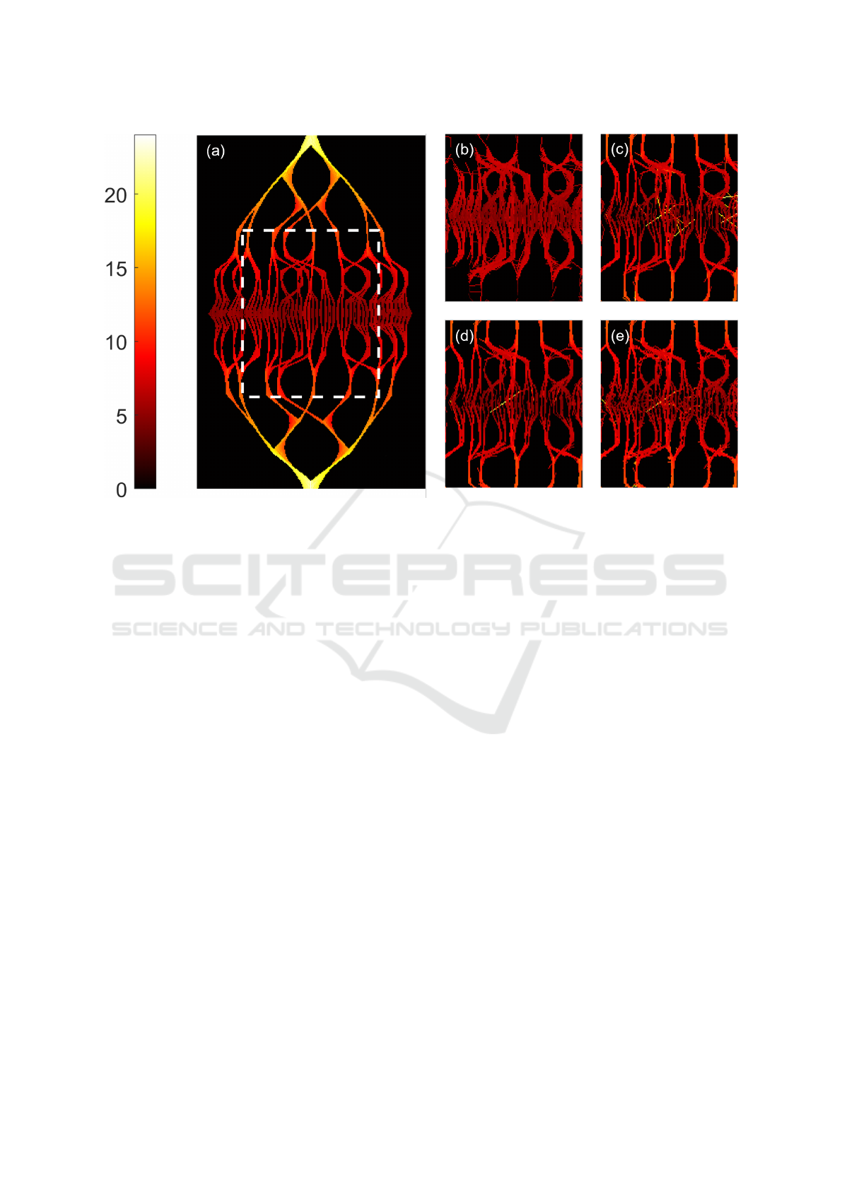
Figure 5: Speed maps of the synthetic vessel network. All are in units of mm/s. 5a: Speed map produced from the ground
truth. The region of interest is enclosed within the white dashed box. 5b: Speed map produced from the tracks generated by
the NN and motion model method. 5c: Speed map produced from the tracks generated using PTNS in R1. 5d: Speed map
produced from the tracks generated using PTNS in R2. Only the straight-line links are plotted. 5e: Speed map produced from
the tracks generated using PTNS in R2. Both the straight and the bending links are plotted. c
ρ
= 0.15 and c
σ
= 1.3 and a
fixed continuity range is used here, with β
1
= 0.5, β
2
= 1.45 and Θ = 45
◦
being used in equation 5.
ier. To assess the full impact of the bending links, we
perform a quantitative analysis of the links, which can
be seen in Table 1.
Table 1 shows the number of true positive links
that a linking method produced (TP) and the total
number of links produced by the method (TL). The
total number of links in the ground truth (GT) is given
in the caption. From these, we calculate two statistics,
precision and Jaccard index, to quantitatively mea-
sure the performance of different linking methods.
From left to right in the table: NN plus motion model
method, PTNS R1, PTNS R2 with straight-line link-
ing, PTNS R2 with bending linking, PTNS R2 with
combined straight-line and bending linking.
We can see that the precision and the Jaccard in-
dex improve as we apply the different elements of
PTNS (columns 2-5 in Table 1). The straight-line
links produced by R1 show high precision, and this
is improved in R2. However, as seen by the Jaccard
index, only ∼33% of the total links in the ground truth
are produced. This inefficient use of the data justifies
the use of the maximum density seeking method to
recover links that have been missed. Combining the
straight-line and bending links in R2 greatly improves
the Jaccard index, recovering ∼50% of ground truth
links. There is a small decrease in the precision due
to the lower precision of the bending links in com-
parison to the straight-line links, which results in the
noise seen in Figure 5e.
3.2 Animal Data Test
We now proceed to test PTNS on an animal data set.
The data was acquired from a sheep ovary using a
1.2mL bolus injection of SonoVue (Bracco, Geneva,
Switzerland) contrast agent. We collected 936 CEUS
frames with a frame rate of 13 Hz. Here, the ground
truth particle locations are no longer available. In
vivo data may have location, architecture and vessel
dimensions available through other techniques. Our
previous work showed that the best ground truth for
in vivo animal data may be acquired through opti-
cal coherence tomography (OCT) (Kanoulas et al.,
2019), where the acquisition is live and vessel features
are preserved and can be directly compared with the
SRUI output. Figure 6 provides the output of PTNS
as described in Figure 2. The original OCT image is
in Figure 5b in (Kanoulas et al., 2019).
The MBs in each CEUS frame have their posi-
tions localised and collected into a MB number map,
Particle Tracking with Neighbourhood Similarities: A New Method for Super Resolution Ultrasound Imaging
35

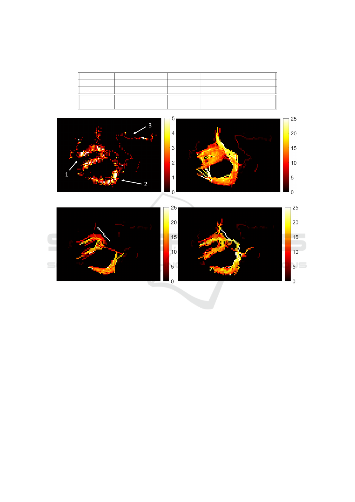
Table 1: Validation results for the synthetic data. TP: number of true positive links produced. TL: total number of links
produced. GT: total number of links in the ground truth. For this synthetic data set, GT = 20040.
NN+MM R1 R2, S links R2, B links R2, S+B links
TP 5800 6008 6856 3531 10387
TL 6820 6728 7109 3881 10990
Precision 0.8504 0.8930 0.9644 0.9098 0.9451
Jaccard (%) 27.54 28.94 33.79 17.32 50.32
(a) (b)
(c) (d)
Figure 6: Tracking results for the sheep dataset. 6a: MB number map. The white arrows indicate the three important structures
in this data set. 6b: Speed map for NN tracking. 6c: Speed map for the links produced by R1. 6d: Speed map for the straight
and bending links produced by R2. All speed maps are in units of mm/s. c
ρ
= 0.5 and c
σ
= 1 and a variable continuity range
was used here, with γ = 1.5 being used in equation 6.
where each pixel (x, y) in the MB number map con-
tains the total number of MBs localised in that pixel
for all image frames, as previously described in Sec-
tion 2.2. This result is shown in Figure 6a. Within the
MB number map, there are three distinct features that
can clearly be seen. These are labeled 1, 2 and 3 in
Figure 6a and they are as follows: a horseshoe shaped
structure, a curved structure, and a thin vessel. Repro-
duction of these three features will be used in place of
the ground truth for this data set to assess the perfor-
mance of PTNS. Just as with the synthetic data, we
use speed maps to show the dynamics and structure,
which will allow us to clearly visualise the results of
each tracking method.
We first apply NN to the sheep data. From Figure
6b, it can clearly be seen that feature 1 is not repro-
duced well. The horseshoe shape is heavily polluted,
which shows that there are many links being made
across the gap in the middle of the structure. Feature
2 is mostly well reproduced, but there are links con-
necting it to feature 1 on the left hand side which are
incorrect. Of the three features, feature 3 is the best
reproduced. In this region, the MB concentration is
low, the speed is low and the structure is thin and well
isolated, which are conditions that NN performs well
in.
Next we apply PTNS to the sheep data. The speed
map for R1 is shown in Figure 6c, and the speed map
for R2 combining straight-line and bending links is
shown in Figure 6d. Features 1 and 2 are better re-
BIOIMAGING 2023 - 10th International Conference on Bioimaging
36

produced using PTNS than they are using NN. The
empty region in the middle of the horseshoe shape
in feature 1 is preserved in Figures 6c and 6d, and
there are no longer any incorrect links connecting the
left of feature 2 to feature 1. However, straight-line
links are not enough to preserve the connection be-
tween features 1 and 2 on the right side of feature
2. Combining straight-line links with bending links
in R2 reproduces this connection. It also further im-
proves the structure of features 1 and 2, which can be
seen in Figure 6d.
The thin vessel in feature 3 is not well reproduced
in Figure 6c. There is a slight improvement in Figure
6d, though there are still parts missing. Because the
MB density is sparse in this region, it is more likely
for links to be rejected due to density assisted linking.
Because of this sparsity of MBs, there isn’t a clear
path of highest MB density for the maximum density
seeking method to follow, and thus it fails to find alter-
native, non-straight-line paths. As a result, this shows
that the maximum density seeking method is not suit-
able for data sets with a very low MB concentration.
3.3 Human Prostate Data
Finally, we apply PTNS to human prostate data.
CEUS data was collected in the Western General Hos-
pital in Edinburgh from patients scheduled for radi-
cal prostatectomy with full ethical approval. An infu-
sion of Luminity
®
(Lantheus, Billerica, USA) contrast
agent was administered to the patient with a roughly
constant flow rate, and data was collected for 3-4 min-
utes at a frame rate of 10 Hz using an iU22 Philips
scanner with C10-3v transducer. The transducer was
secured in place, scanning a region suspected to con-
tain cancer from prior MRI assessment. The ground
truth here refers to the structure and location of the tu-
mour as determined by histopathological evaluation.
In comparison to the sheep data, this no longer speci-
fies the vessel dimensions and architecture but rather
the approximate topography of the tumour, though the
results may not perfectly match the histopathology
given the orientation of the ultrasound frame. Fig-
ure 7 shows the results of PTNS when applied to the
prostate data.
Figure 7a is the B-mode prostate image of the pa-
tient under investigation, where the prostate border is
circled with a yellow line. The histopathology results
are shown in Figure 7b. Here the cancer is encir-
cled by the black line. This was then matched onto
SRUI images, taking into account the shape distor-
tion due to the ultrasound scanner. We now apply
PTNS to track the MBs in the CEUS data, begin-
ning with R1. The track number map for R1, which
is the number of tracks passing through each pixel,
is shown in Figure 7c while the corresponding speed
map is shown in Figure 7d. The cancer region has
been identified by our pathology team and is encir-
cled by the blue dashed line in Figure 7c. As seen,
the cancer region has both a high track number and a
high speed. We note that high track number and high
speed is also found in healthy areas, noticeably in the
central region. However, there are no particular spa-
tial structures in the cancer region compared to those
in healthy areas.
We further apply R2 of PTNS, with a variable con-
tinuity range as defined by equation 6. Results with
different continuity levels have been investigated by
adjusting the control parameter γ. Figures 7e and 7f
are the track number map and the speed map for R2
with γ = 1.5. Comparing Figure 7e with Figure 7c,
it can clearly be seen that the total number of tracks
in the prostate is reduced in R2, which also shows
clearer structures due to the imposed continuity re-
strictions. Similar features due to continuity restric-
tions are also observed when comparing Figure 7f
with Figure 7d.
From the literature, it is known that the vascula-
ture of prostate cancer is different than that of healthy
tissue (Forster et al., 2017; Alizadeh et al., 2013; Vau-
pel and Kelleher, 2012). Cancer blood vessels are
typically thicker than healthy blood vessels (Forster
et al., 2017; M
¨
uller et al., 2008), with increasingly
tortuous vessels (Alizadeh et al., 2013) and a het-
erogeneous blood flow (Vaupel and Kelleher, 2012;
Jochumsen et al., 2020). As such, we expect some
discrepancies in the structures and dynamics between
the cancer region and healthy region when the conti-
nuity range varies. In order to quantify this, a com-
parison between the number of tracks in the cancer
and healthy regions at different levels of continuity
restrictiveness is investigated. Table 2 compares the
track number in the cancer and healthy regions of the
patient for R1, and R2 with two different γ values.
As seen in Table 2, while both the cancer and
healthy region shows a decrease in the number of
tracks as the continuity range becomes more restric-
tive, the cancer region shows a greater reduction in
track number; 70% compared to 75% for γ = 1.5,
and 25% compared to 34% for γ = 1. The larger re-
duction in track number in the cancer region shows
that this region lacks motion continuity more than the
healthy region. This in turn indicates that the vessels
and corresponding blood flow in cancer regions be-
have more chaotically in structure and dynamics re-
spectively. This finding is in line with literature ob-
servations of prostate cancer blood vessels (Alizadeh
et al., 2013; Vaupel and Kelleher, 2012; Jochumsen
Particle Tracking with Neighbourhood Similarities: A New Method for Super Resolution Ultrasound Imaging
37

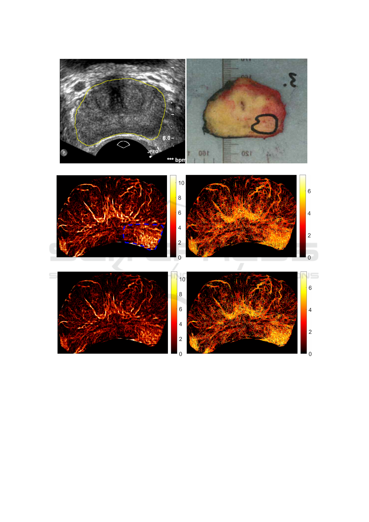
(a) (b)
(c) (d)
(e) (f)
Figure 7: PTNS results for the human prostate data set. 7a shows a B-mode image with the prostate enclosed by the yellow
line. 7b shows the results of the histopathology. 7c shows the track number map for R1. The area enclosed by the blue dashed
line is the cancer region. 7d shows the speed map for R1, in units of mm/s. 7e shows the track number map for R2. 7f shows
the speed map for R2, in units of mm/s. c
ρ
= 0.15 and c
σ
= 1.3 and a variable continuity range was used here, with γ = 1.5
being used in equation 6.
et al., 2020). These findings show that PTNS can po-
tentially be a useful tool to identify distinctive struc-
tural and dynamical features in cancer areas to assist
in the diagnosis of prostate cancer.
4 CONCLUSIONS
In this paper, we proposed a new method which we
call Particle Tracking with Neighbourhood Similar-
ities which seeks to address the issues of incorrect
BIOIMAGING 2023 - 10th International Conference on Bioimaging
38

Table 2: Table showing how the number of tracks generated for the human prostate data set reduce as the strictness of the
continuity range increases, presented as the raw number of tracks and also as percentage of the tracks generated in R1. The
tracks in the cancer and healthy regions have been separated to show the difference in behaviour.
Cancer Tracks % of R1 Healthy Tracks % of R1
R1 10386 100 46832 100
R2, γ = 1.5 7309 70.37 35379 75.54
R2, γ = 1 2569 24.74 15717 33.56
linking between vessels and the first link in a track
identified in current particle linking approaches and
methods when applied to CEUS images. In synthetic
data, we have shown that PTNS improves the perfor-
mance of particle tracking. PTNS uses the data more
efficiently as a result of increasing the precision and
Jaccard index. In animal data, we have demonstrated
that PTNS can construct complex structures of in vivo
data, particularly in regions of high MB density.
Finally, we have applied PTNS to human prostate
data to investigate the structure and dynamics of the
vasculature for a patient with prostate cancer. Be-
cause PTNS is a two run process, the second run can
be used to probe different levels of motion continuity
by varying the control parameters, which can provide
the means to distinguish different blood flow dynam-
ics between cancer and healthy tissue. Using this ap-
proach, we observe that the cancer region exhibited a
more chaotic vascular structure, resulting in a larger
decrease in track number when the velocity continu-
ity was made more restrictive. This is consistent with
the current understanding of prostate cancer. More
broadly, this result shows that super resolution ultra-
sound imaging of prostate cancer can potentially be
developed into tools for diagnosis and focal therapy.
ACKNOWLEDGEMENTS
We would like to thank Lantheus Medical Imaging,
Inc. for providing the Luminity
®
contrast agent as part
of their Research Grants program. We would also like
to thank the Western General Hospital Edinburgh the-
atre team for their time and for allowing us to use their
facilities.
REFERENCES
Alizadeh, F., Hadi, M., Khorrami, M., Yazdani, M.,
Joozdani, R., Tadayyon, F., and Mellat, M. (2013).
Prostate cancer: Relationship between vascular diam-
eter, shape and density and gleason score in needle
biopsy specimens. Advanced Biomedical Research,
2(1).
Betzig, E., Patterson, G., Sougrat, R., Lindwasser, O.,
Olenych, S., Bonifacino, J., Davidson, M., Lippincott-
Schwartz, J., and Hess, H. (2006). Imaging intracellu-
lar fluorescent proteins at nanometer resolution. Sci-
ence, 313(5793):16–42–1645.
Brown, J., Christensen-Jeffries, K., Harput, S., Zhang,
G., Zhu, J., Dunsby, C., Tang, M., and Eckersley,
R. (2019). Investigation of microbubble detection
methods for super-resolution imaging of microvas-
culature. IEEE Transactions on Ultrasonics, Ferro-
electrics, and Frequency Control, 66(4):676–691.
Chenouard, N., Smal, I., de Chaumont, F., Ma
ˇ
ska, M.,
Sbalzarini, I., Gong, Y., Cardinale, J., Carthel, C.,
Coraluppi, S., Winter, M., Cohen, A., Godinez, W.,
Rohr, K., Kalaidzidis, Y., Liang, L., Duncan, J., Shen,
H., Xu, Y., Magnusson, K., Jald
´
en, J., Blau, H., Paul-
Gilloteaux, P., Roudot, P., Kervrann, C., Waharte, F.,
Tinevez, J., Shorte, S., Willemse, J., Celler, K., van
Wezel, G., Dan, H., Tsai, Y., de Sol
´
orzano, C., Olivo-
Marin, J., and Meijering, E. (2014). Objective com-
parison of particle tracking methods. Nature Methods,
11(3):281–289.
Couture, O., Hingot, V., Heiles, B., Muleki-Seya, P.,
and Tanter, M. (2018). Ultrasound localisation mi-
croscopy and super resolution: a state of the art. IEEE
Transactions on Ultrasonics, Ferroelectrics, and Fre-
quency Control, 65(8):1304–1320.
Errico, C., Pierre, J., Pezet, S., Desailly, Y., Lenkei, Z., Cou-
ture, O., and Tanter, M. (2015). Ultrafast ultrasound
localisation microscopy for deep super-resolution vas-
cular imaging. Nature, 527(7579):499–502.
Forster, J., Harriss-Philips, W., Douglass, M., and Bezak, E.
(2017). A review of the development of tumor vascu-
lature and its effects on the tumor microenvironment.
Hypoxia, 5:21–32.
Genovesio, A., Liedl, T., Emiliani, V., Parak, W., Coppey-
Moisan, M., and Olivo-Marin, J. (2006). Multiple par-
ticle tracking in 3-d+t microscopy: method and appli-
cation to the tracking of endocytosed quantum dots.
IEEE Transactions on Image Processing, 15(5):1062–
1070.
Godinez, W., Lampe, M., W
¨
orz, S., M
¨
uller, B., Eils, R.,
and Rohr, K. (2009). Deterministic and probabilistic
approaches for tracking virus particles in time-lapse
fluorescence microscopy image sequences. Medical
Image Analysis, 13(2):325–342.
Hess, S., Girirajan, T., and Mason, M. (2006). Ultra-
high resolution imaging by fluorescence photoactiva-
tion localisation microscopy. Biophysical Journal,
91(11):4258–4272.
Jochumsen, M., S
¨
orensen, J., Pederson, B., Nyengaard, J.,
Krag, S., Frøkiær, J., Borre, M., Bouchelouche, K.,
Particle Tracking with Neighbourhood Similarities: A New Method for Super Resolution Ultrasound Imaging
39

and Tolbod, L. (2020). Tumour blood flow for predic-
tion of human prostate cancer aggressiveness: a study
with rudibium-82 pet, mri and na+/k+-atpase-density.
European Journal of Nuclear Medicine and Molecu-
lar Imaging, 48(2):532–542.
Kanoulas, E. (2020). Methodology for a Super-Resolution
Contrast-Enhanced US 2D-Imaging for Clinical Di-
agnosis. PhD thesis, Heriot Watt University.
Kanoulas, E., Butler, M., Rowley, C., Voulgaridou, V.,
Diamantis, K., Duncan, W., McNeil, A., Averkiou,
M., Wijkstra, H., Mischi, M., Wilson, R., Lu, W.,
and Sboros, V. (2019). Super-resolution contrast-
enhanced ultrasound methodology for the identifica-
tion of in vivo vascular dynamics in 2d. Investigative
Radiology, 54(8):500–516.
Lin, F., Rojas, J., and Dayton, P. (2016). Super resolution
contrast ultrasound imaging: Analysis of imaging res-
olution and application to imaging tumor angiogene-
sis. In 2016 IEEE International Ultrasonics Sympo-
sium (IUS).
Mazzaferri, J., Roy, J., Lefrancois, S., and S., C. (2014).
Adaptive settings for the nearest neighbour particle
tracking algorithm. Bioinformatics, 31(8):1279–1285.
M
¨
uller, B., Lang, S., Dominietto, M., Rudin, M., Schulz,
G., Deyhle, H., Germann, M., Pfeiffer, F., David,
C., and Weitkamp, T. (2008). High-resolution tomo-
graphic imaging of microvessels. Developments in X-
Ray Tomography VI.
Opacic, T., Dencks, S., Theek, B., Piepenbrock, M., Acker-
mann, D., Rix, A., Lammers, T., Stickeler, E., De-
lorme, S., Schmitz, G., and Kiessling, F. (2018).
Motion model ultrasound localization microscopy for
preclinical and clinical multiparametric tumor charac-
terization. Nature Communications, 9(1).
Sboros, V. (2008). Response of contrast agents to
ultrasound. Advanced Drug Delivery Reviews,
60(10):1117–1136.
Tang, S., Song, P., Trzasko, J., Lowerison, M., Huang,
C., Gong, P., Lok, U., Manduca, A., and Chen,
S. (2020). Kalman filter-based microbubble track-
ing for robust super-resolution ultrasound microvessel
imaging. IEEE Transactions on Ultrasonics, Ferro-
electrics, and Frequency Control, 67(9):1738–1751.
Vaupel, P. and Kelleher, D. (2012). Blood flow and oxy-
genation status of prostate cancers. Advances in Ex-
perimental Medicine and Biology, pages 299–305.
Xu, H. (2009). Contrast-enhanced ultrasound: the evolving
applications. World Journal of Radiology, 1(1):15–24.
Yang, L., Qiu, Z., Greenaway, A., and Lu, W. (2012). A new
framework for particle detection in low snr fluores-
cence live cell images and its application for improved
particle tracking. IEEE Transactions on Biomedical
Engineering, 59(7):2040–2050.
BIOIMAGING 2023 - 10th International Conference on Bioimaging
40