Synchronizing Vehicle Routing and Photo-Voltaic Production

Alejandro Olivas Gonzalez, Alain Quilliot and Hélène Toussaint

Labex IMOB3, LIMOS Laboratory, UCA/CNRS, Cézeaux Campus, Clermont-Ferrand, France

Keywords: Routing, Scheduling, Bilevel Optimization, Machine Learning.

Abstract: We deal here with the routing and scheduling of electric vehicles in charge of performing internal logistic

tasks inside some protected area. Some vehicles are provided in energy by a local photo-voltaic facility with

limited production/storage capacities and time dependent production rates. In order to avoid importing energy

from outside (notion of self consumption) one must synchronize energy consumption and production while

minimizing both production and routing costs. Because of the complexity of resulting bi-level optimization

model, we handle it while shortcutting the production scheduling level with the help of surrogate estimators,

whose values are computed through a pricing mechanism and machine learning devices. According to this

purpose we design, implement and test several algorithms and get an evaluation of the potentiality of such

surrogate component based approaches. This work was carried on in partnership with national power company

EDF, in the context of the PGMO program.

1 INTRODUCTION

The notion of multi-level decisional (Caprara, 2014;

Chen, 2013; Colson, 2005; Dempe, 2015) model is

mainly related to situations when decision is shared

between several players, independent from each other

or tied together by some hierarchical or collaborative

link. Then, solving such a model aims at providing a

best scenario in case all the players accept to submit

themselves to a common authority (centralized

paradigm), or, if it is not the case (collaborative

paradigm), at helping them into the search for a

compromise (Kleinert, 2021). Standard approaches

involve decomposition schemes, which may be

hierarchical (Benders decomposition, Stackelberg

equilibrium,…) or transversal (Lagrangean

relaxation). Still in both case some major difficulties

remain: They are related to the sensitivity issue, which

means the way one may retrieve information from the

different levels in order to make them interact, and to

the collaborative issue, which may impose the players

to deal with incomplete information. It comes that a

trend, boosted by the rise of machine learning

technology (Krystow, 2018; Wojtuziak, 2012), is to

bypass some levels of the global model and replace

them by surrogate estimators, likely to approximate

the constraints and costs induced by the decisions

taken at those levels.

It is this point of view which we adopt here while

dealing with the joint management of local

photovoltaic energy production by a PV-facility

(Luthander, 2015; Smart Together, 2016) and its

consumption by a fleet of electric vehicles in charge

of logistic tasks inside a restricted area. This problem

arose in the context of the activities of IMOBS3

(Innovative Mobility) Labex in Clermont-Ferrand,

which conducts research on both autonomous electric

vehicles and solar energy, and of the national PGMO

program promoted by power company EDF. The fact

is that both market deregulation and emergent

technologies currently induce the rise of local

renewable energy producers (factories, farms and

even individual householders) who simultaneously

remain consumers (Balbiyad, 2019; Deb, 2018;

Grimes, 2008) and so make self-consumption become

an issue. A key operational feature of self-

consumption management happens to be the need for

synchronization between strongly time-dependent

energy production and its consumption.

So we consider here, on one side, a production

manager who runs a PV (Photo-Voltaic)-Plant, which

not only distributes energy between end-users

(electric vehicles) but also buys and sells energy on

the market. On the other side, we consider a fleet

manager who schedules and routes electric vehicles in

such a way that they efficiently achieve a set of

internal logistic tasks. Both interact through

Gonzalez, A., Quilliot, A. and Toussaint, H.

Synchronizing Vehicle Routing and Photo-Voltaic Production.

DOI: 10.5220/0011612500003396

In Proceedings of the 12th International Conference on Operations Research and Enterprise Systems (ICORES 2023), pages 127-134

ISBN: 978-989-758-627-9; ISSN: 2184-4372

 2023 by SCITEPRESS – Science and Technology Publications, Lda. Under CC license (CC BY-NC-ND 4.0)

127

recharging transactions: In order to avoid that the

vehicles waste time while waiting for their battery to

be recharged, the PV-Plant relies on a set of identical

batteries, so that the vehicles only need to move

toward the PV-Plant and switch batteries in order to

be recharged. This plug out/in operation is

instantaneous. But limited storage and recharge

capacities impose both players to carefully

synchronize the strongly time-dependent energy

production and its consumption. This synchronization

requirement makes resulting bi-level decision

problem complex, even if we restrict ourselves to the

centralized paradigm. Though many searchers have

recently showed interest into the decisional problems

which may be related to the management of renewable

energy, they most often focused either on production

control and scheduling (Adulyasak, 2012 ; Irani, 2003,

Erdelic, 2019) or on the issues related to power

consumption (Albrecht, 2013; Koc, 2019), without

dealing with this synchronization issue (Bendali,

2021; Trotta, 2022). Our goal here is to address it by

shortcutting the part of the process related to

production management and handling the vehicle

routing master level while using a surrogate

formulation of the cost and constraints related to

production. We try two approaches: the first one is

based upon a parametric pricing mechanism; the

second involves a convolutional neural network. We

suppose, for the sake of simplicity, that our system

behaves in a deterministic way.

The paper is organized as follows. We first

(Section 2) introduce the PV_Prod_VRP problem.

We set it according to the MILP (Mixed Integer

Linear Programming) framework and discuss

different formulations. Next (Section 3), we present

the 3-step algorithmic framework for the handling of

PV_Prod_VRP through the use of surrogate

estimators. In Section 3.1 we provide the details of a

Branch and Cut algorithm which performs (Step 1)

the computation a collection of elementary trips; In

Section 3.2 we specify the surrogate estimators of the

production cost which we use in order to schedule the

elementary trips (Step 2): the first one relies on a

parametric pricing mechanism while the second one

involves a convolutional neural network. Section 4 is

devoted to numerical experiments.

2 THE PV_PROD_VRP PROBLEM

We consider a fleet of K small identical electric

vehicles initially located at a depot Depot = 0 and

which are required to perform VRP: Vehicle Routing

Problem tours, that means to visit a set of stations J =

{1,…, M} within a time horizon [0, TMax]. Moving

from station j to station k requires 

j,k

time units and

an amount E

j,k

of energy. Recharge transactions take

place at Depot. In order to avoid that the vehicles wait

every time they recharge, the fleet relies on a set B of

identical batteries, with capacity C and charge speed

CS, and vehicles may switch their battery every time

they come back to Depot. This plug out/in operation is

considered as almost instantaneous. It comes that

while the vehicles are running with active batteries,

idle batteries are recharged at Depot before being used

again by the vehicles. For any battery b in B, V

denotes its initial load. We call elementary trip any

VRP sub-tour that a vehicle may perform without

recharging: such an elementary trip is a sequence

{Depot = j

, j

,…, j

, j

s+1

= Depot} such that the sum



j,Succ(j)

does not exceed capacity C.

In order to implement a self-consumption policy,

Depot is provided with a PV-Plant, that means with a

photovoltaic facility which assigns the batteries to the

vehicles and produces its own energy that it distributes

between the currently idle batteries or that it sells to

the market. In case this self-produced energy is not

enough, the PV-Plant can also buy energy to the

market. The time space [0, TMax] being divided into

small periods i = 1,…, N, all with same length p, we

denote by C

the recharge capacity, i.e the energy

which may be loaded into a battery during 1 period.

We also denote by R

the expected production of the

PV-Plant at period i, by A

the energy unit purchase

price at period i, and by B

the energy unit sale price.

Clearly we have, for any i, A

≥ B

. Figure 1 describes

the way the PV-Plant and the vehicle fleet interact.

Figure 1: The Global Self-Consumption System.

Resulting PV_Prod_VRP problem comes as follows:

PV_Prod_VRP Problem: {Simultaneously schedule

the vehicle fleet and the activity of the PV-Plant, in

such a way that:

 Every station is visited once;

ICORES 2023 - 12th International Conference on Operations Research and Enterprise Systems

128

 Every time a vehicle k comes back to Depot,

the PV-Plant assigns it a battery loaded to

make possible its next elementary trip;

 The global energy load of the batteries at the

end of period N must be at least the same as at

the beginning of the process.

 Some global cost is minimized, which

combines standard VRP cost with the

difference between the energy purchase cost

and the profit derived from energy sales}.

In order to formalize, let us first suppose that the

vehicles have been scheduled, which means that a

collection 

of elementary trips  has been

computed and each  scheduled inside a set of

consecutive periods I(). We denote by 

= {(,

I()),   

} the resulting set of scheduled trips  =

{(, I()). For any trip , we denote by E() its energy

consumption, by T() its duration, by S() its set of

stations, by E

Mean

() the quotient E()/Card(I()),

and we extend those notations to scheduled trips .

Then, PV_Prod sub-problem is about the way the PV-

Plant loads the batteries and assigns them to

scheduled trips :

ILP PV_Prod(



) MILP (Mixed Integer Linear

Program ) Model:

{Compute

 {0, 1}-vector U = (U



,  



, b  B): U



= 1 iff b = b() is the battery assigned to ;

 {0, 1}-vector  = (

b,i

, b  B, i = 1,…, N):



b,i

= 1 iff b is idle at period i;

 X

= (X

, i = 1,…, N), X

= (X

, i = 1,…, N),

= (X

b,i

, b  B, i = 1,…, N), which

respectively denote the energy bought, sold

and distributed to battery b, by the PV-Plant;

 W = (W

b,i

, b  B, i = 0,…, N): W

b,i

is the

energy inside battery b at the end of period i.

Objective Function: Minimize



- 

Constraints:

 For any b, i, W

b,i

≤ C

and X

b,i

≤ C

.

b, I

; (R1)

 For any b, W

b,0

= V

; (R2)

 

b,N

≥ 

; (R3)

 For any i,

+ X

= X

+ 

b,i

; (R4)

 For any b  B, i:

(1 - 

b, i

) = 



s.t i





)



≤ 1; (P1)

 For any  



, 



= 1; (P2)

 For any b  B, i: W

b,i

= W

b,i-1

+ X

b,i

- 



s.t i





)

Mean

().U



. (P3)}

Explanation: (R1) means that we charge a

battery b only if it is idle. (R3) imposes the batteries

to be globally loaded with at least as much energy at

the end of the whole process as at the beginning. (R4)

tells the way energy is distributed between sale,

purchase and battery loading. (P1) means that b is

active at period i only if has been assigned to a unique

scheduled trip , active at period i. (P2) says that any

scheduled trip  is assigned a unique battery b. (P3)

describes the evolution of a battery b from a period i

- 1 to next period i.

We may now formalize our global PV_Prod_VRP

problem. The VRP decision makes our K vehicles visit

at least once any station j in {1,…, M) and means a

collection 

of scheduled trips  = (, I()) such that:

 For any i, Card({  

s.t i  I()} ≤ K. (S1)

 For any j, Card({  

s.t j S()} ≥ 1. (S2)

If we consider as standard VRP cost of 

the

global riding time 



T() (Driver Cost) then, a time

versus money coefficient  being given, our

PV_Prod_VRP problem comes as follows:

PV_Prod_VRP Problem: {Compute a collection 

of scheduled trips, such that (S1, S2) hold and which

minimizes the sum .(







T()) +

Val_PV_Prod(

), where Val_PV_Prod(

) is the

optimal PV_Prod(



) value}.

Denoting by  the set of all possible scheduled

trips allows us to propose the following MILP

formulation of PV_Prod_VRP:

PV_Prod_VRP MILP Formulation:

{Compute:

 {0, 1}-vector Z = (Z



,   }: Z



= 1 means

that we select scheduled trip ;

 X

, X

, W, U and  as in above PV_Prod

MILP model;

Objective Function:

Minimize 

- 

+ .



T().Z



;

Constraints:

 (R1,…, R4, P1, …, P3) of PV_Prod;

 For any i = 1,…, N, 



s.t i





)



≤ K; (S1)

 For any j = 1,…, M, 



s.t j





)



≥ 1. (S2)

 For any  , 



= Z



; (S3)

Explanation: (S3) means that any selected scheduled

trip must be assigned a battery.

An Example: Let us consider a customer set X = {A,

B, C, D, E} and 2 vehicles v

and v

, which follow

routes 

and 

as in figure 3 below: Numbers above

Synchronizing Vehicle Routing and Photo-Voltaic Production

129

every arc respectively represent the time and the

energy required in order to traverse the arc.

Figure 2: Routes



and



We also suppose that: we are provided with 2

identical batteries b

and b

, both with capacity C =

12 and with initial loads respectively equal to 7 and

6; the time space is divided into 10 periods, all with

duration equal to 2; recharge capacity C

is equal to

3 and production data come as in table 1 below:

Table 1: PV Prices and Production Coefficients.

i 1 2 3 4 5 6 7 8 9 10

2 3 7 7 3 2 6 7 4 2

1 2 4 4 1 1 3 3 2 1

4 4 3 5 2 6 4 4 4 5

Then we derive a feasible solution from 

and 

 

starts at time 4 with battery b

, comes back to

Depot at time 9, waits in Depot until time 14

and starts until time 18 with battery b

;

 

starts at time 2 with battery b

, comes back to

Depot at time 6, waits in Depot until time 12 and

starts again with battery b

until time 16.

 Vectors X

, X

and X

are given by table 2 below:

Table 2: Solution Values.

i 1 2 3 4 5 6 7 8 9 10

1 0 0 0 1 0 0 0 0 1

0 1 3 2 0 0 1 4 2 0

b1,i

2 * * 3 3 3 3 * * 3

b2,i

3 3 * * * 3 * * 2 3

Time versus money coefficient  is equal to 2.

Related cost is: 2*17 (Vehicle Time Cost) + 5

(Energy Purchase) - 43 (Energy Sale) = - 4. We earn

38 money units, under a riding time of 17.

A Short Discussion: Variants of the PV_Prod

Model. In practice, production configurations may be

more complex. Let us mention here two variants:

First variant: Batteries remain identical, but may be

used in order to store energy and next sell it.

According to this hypothesis, a battery b may

receive energy at period i and sell it at period i’ > i.

The Recharge model must be updated through the

introduction of an additional vector Y

= (Y

b,i

, b  B,

i = 1,…, N), which means the amount of energy sold

at any period i by battery b.

Second variant: A fixed storage unit is added to the

PV-Plant, which may be used either for sale or for

battery feeding when energy is scarce or expensive.

According to this hypothesis, such a Buffer

battery BUFF, with storage capacity C

BUFF

, initial

load V

BUFF

, recharge capacity C

R_BUFF

and discharge

capacity C

D-BUFF

, induces the introduction of the

following variables into the Recharge model:

 X

BUFF

= energy sent from the PV-Plant to the

Buffer battery at i;

 X

B_BUFF

= energy sold by the Buffer battery at i;

 Y

BUFF

b,i

= energy sent by the Buffer battery to

battery b at i;

 W

BUFF

= energy inside the Buffer battery at the

end of i.

3 PV_PROD_VRP HANDLING:

SURROGATE COMPONENTS

PV_PROD_VRP is a complex model, with 3 discrete

decision levels, respectively related to elementary

trips, scheduled trips, and batteries. Its MILP

formulation is hardly practicable and would badly fit

true life contexts, where decisions related to

respectively vehicles and the PV-Plant are likely to

depend on distinct players. Instead, we propose 2

approaches:

First approach: Solving above PV_Prod_VRP

MILP model, while restricting ourselves to a pre-

computed set  of scheduled trips.

Second Approach: Solving the PV_Prod_VRP bi-

level model, while partially short-cutting the slave

PV_Prod level through the introduction of surrogate

constraints and criteria.

It is this second approach which we follow here.

3.1 Shortcutting the PV_Prod Level

Our purpose here is to compute the scheduled trip set



without explicitly involving the PV-Plant. But,

while the schedule  -> I() must take into account

prices A

, B

and production rates R

, we can only say

that a well-fitted collection 

requires small amounts

of both time and energy. So we should split the

routing part of the problem (computing the

elementary trips) from its scheduling part (scheduling

those elementary trips). This leads us to the following

parametric VRP_Surrogate process:

ICORES 2023 - 12th International Conference on Operations Research and Enterprise Systems

130

VRP_Surrogate Parametric Algorithm: Initialize

flexible scaling parameter ; Not Stop; Current best

solution Best_Sol is undefined;

While Not Stop do

step: Compute an elementary trip collection 

which minimizes .







T() + . 







E(),

step: Turn 

into a scheduled trip collection



, i.e compute intervals I(),   

in a way

which meets some surrogate constraints

(SURR) and which minimizes some surrogate

cost ( -> I());

step: Update  and Stop; Solve PV_Prod(

)

and update Best_Sol; .

3.2 Step 1: Branch and Cut

Trying exact methods leads to set an ILP model. For

any subset A  J = {1,…, M}, we set 

(A) = {arcs (j,

k) such that j  A and k  A} and Cl(A) = {arcs (j, k)

s.t at least j or k is in A}. We get the following

Elementary_Trip ILP model, which involves a

specific SNS: Strong No Sub-Tour Constraint:

Elementary_Trip ILP model:

{Compute a (0, 1)-valued vector Z = (Z

j,k

, j, k =

0,…, M) in such a way that :

 For any j, 

j,k

= 

j,k

= 1; (S2)

 For any subset A of {1, …, M}, (SNS)

C.(

(j, k )





+(A)

j,k

) ≥ 

(j, k )



Cl( A)

j,k .

j,k

 Minimize .(

j,k

. T

j,k

,) + .(

j,k

. E

j,k

,).

The explanation of above (SNS) constraint comes

with the statement below:

Theorem 1: {0, 1} vector Z meets (S2, SNS) iff arcs

(j, k) such that Z

j,k

= 1 define a collection







of sub-

tours



, …,



, with S = 

0,k

= such that:

 For every s = 1,…, S,



starts from Depot = 0

and ends into Depot, and requires an energy

amount no more than C;

 Every station j is visited exactly once by

collection









Constraints SNS may be separated in polynomial

time through a max flow (min cut) procedure.

Sketch of the Proof: Constraints (SNS) imply that Z

gives rise to a collection  of sub-tours 

, …, 

which globally involve exactly once any station j, and

which all contain Depot = 0 (No Sub-Tour). If some

tour 

spends more energy than capacity C, then a

subset A of {0, …, M+1} exists which makes Z violate

(SNS). We deduce the first part of our statement. As

for the second part, we see that, some vector Z

(integral or rational) being given, separating (SNS)

means searching for B = {0, 1, …, M} – A, such that:



j,k



j,k

C(

(j, k )





+(B)

j,k

) < 

= 

j,k

 (*)

In order to do it, we construct a network G

Aux

whose node set is{0, 1, …, M+1) and whose arc set

Aux

may be written U

Aux

= U  Copy(U) with:

o U = {(j, k), j, k = 0,…, M, such that Z

j,k

≠ 0:

provided with a capacity w

= Z

j,k

.(C

- E

j,k

)};

o With any arc e = (j, k) in U, we associate an arc

u = Copy(e) = (j, M+1) provided with a capacity

= Z

j,k

. Then arc set Copy(U) is the set of

all arcs Copy(e), e  U.

But searching for B such that (*) means searching

for B  { 0, 1, …, M}, such that:





UAux, s.t (origin(u)





(destination(u)



< .

It is known that, in case B exists, it may be

retrieved through the standard Min Cut algorithm. 

Theorem 1 and related proof provide us with an

efficient separation procedure which opens the way

to the implementation of a Branch and Cut process.

3.3 Step 2: Surrogate Components

In order to enhance PV_Prod(

) feasibility, we

impose the following surrogate necessary (but not

sufficient) constraints:

 For any period i, Card({  

such that i 

I()}) ≤ K. (S1)

 For any i

= 1,…, N: C

.(

i ≤ i0-1

.n(



, i)) +



≥ 



s.t Start(



) ≤ i0

.E(),

where n(



, i) is the number of scheduled trips 

idle at period i, and Start() is the starting period of

, and which means that we must be able to feed the

batteries in such a way that the trips becomes

possible. (SURR2)

Then, in order to make possible the use of any

surrogate estimator ( -> I()), we implement Step

2 while relying on a non deterministic local search

heuristic Scheduled_Trip(

,  ). So, what remains

to be done is to discuss estimator .

3.3.1 Defining (

) According to a Pricing

Mechanism

The idea here is that the cost of a schedule ( -> I())

is determined by the distribution of resulting values

n(

, i), which means, for any period i, the number of

batteries which are available for recharge at i. Let us

denote by E = (



E()) the global charge which

has to be loaded into the batteries and by I = (



T()/p) the number of periods required in order to

perform all trips of 

. The point is that if we suppose

Synchronizing Vehicle Routing and Photo-Voltaic Production

131

that all batteries receive a same charge E

Mean

= E/I at

every period when they are idle, then we get the cost

of the production process through the following

formula: Cost = I.Q

Stand

i, n(



, i)

, where standard price

Stand

i, n

for the recharge of n idle batteries at period i

is given by:

Stand

i,n

= A

.(n.E

Mean

– R

) if n.E

Mean

≥ R

and Q

Stand

i,n

= B

.(n.E

Mean

– R

) else.

Clearly, the energy amount loaded into an idle

battery b at period i may differ from E

Mean

. Still, above

reasoning suggests us to express the surrogate cost

( -> I()) = (



) involved into the

VRP_Surrogate algorithm as a sum 

i, n(



, i)

, where

i,n

is the estimation of the cost induced by n batteries

in recharge (idle) at period i. Besides, we notice that:

 If n(

, i).E

Mean

≥ R

, then Q

i,n

should increase

with A

;

 If n(

, i).E

Mean

≤ R

, then Q

i,n

should decrease

as B

increases.

This leads us to set:

 A

Mean

= mean value A

, i = 1,…, N; B

Mean

= mean

value B, i = 1,…, N;

 Q

i,n

= Q

Stand

i,n

.(1 + 



.(A

– A

Mean

)) if

n(

, i).E

Mean

(

) ≥ R

and else Q

i,n

= Q

Stand

i,n

.(1 + 



.(B

– B

Mean

)),





, 



being non negative flexible parameters.

3.3.2 Computing (

) Through a Neural

Network

Instead of relying on energy price coefficients Q

i,n

, we

use a neural network N_Energy in order to evaluate a

scheduled trip collection 

. N_Energy is

implemented with the help of the TensorFlow open

software and trained with a large number (4000) of

PV_Prod(



) instances. It is designed as a

convolutional neural network. Such a network, whose

main purpose is to be adaptable to inputs with flexible

sizes, usually works in 2 (or more) steps: In the first

step, a same standard perceptron CM called

convolutional mask, is applied to fixed size neighbors

of the components of the input vector IN = (IN

, m 

M), and yields an output vector OUT = (OUT

, m 

M); In the next step, a pooling mechanism is applied

to Out, in order to compact it into the fixed size input

of another perceptron N_Pool which computes the

final output. In the present case this final output is a

number  between 0 and 1, whose semantics are that

it should be possible to express the optimal value

VAL_PV_Prod(

) of PV_Prod(

) as a sum

Val_Min + .(Val_Max – Val_Min), where Val_Max

and Val_Min are respectively a lower bound and an

upper bound of VAL_PV_Prod(

). More precisely,

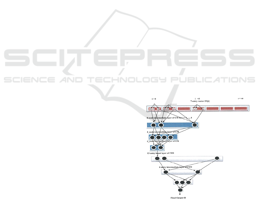
the main components of N_Energy are (see fig. 3):

Input layer: For any input 

, A, B, R, V of the

PV_Prod problem, we homogenize it as a (N+1).7

vector IN, with IN[i] = (A*

, B*

, R*

, *

, Q

, C*,

*), with:

 NA*

= A

Mean

; B*

= B

Mean

, where A

Mean

Mean value of the coefficients A

, i = 1,…, N;

 *

= 



s.t i





)

Mean

(); *

= 0;

 R*

= R

Mean

; *

= 

Mean

, where R

Mean

= Mean

value of coefficients R

; R*

= (

)/R

Mean

;

 Q

= n(

, i)/Card(B);

 C* = C/R

Mean

; C

* = C

Mean

Convolutional mask: CM works on any sub-vector

IN*

= (IN[i], …, IN[i+4]), which means an input with

35 input arcs. It contains 3 inner layers, respectively

with sizes 8, 4 and 2, and ends into an output layer,

with 1 input value OUT

. All 322 synaptic arcs are

allowed, together with standard biased sigmoid

activation functions whose derivative value in 0 is

equal to ½. .

The pooling mechanism: works by merging

consecutive values OUT

into a single value, in such

a way that we get an intermediate vector AUX, with

13 entries, all with values between 0 and 1.

Final Perceptron N_Pool: Once the pooling

mechanism has been applied, we handle resulting 13

dimensional vector AUX with a perceptron N_Pool,

with input layer with size 13, intermediate layers with

size 6 and 3, and a final layer with size 1.

Figure 3: The Neural Network N_Energy.

This network is complete in the sense that all 99

synaptic arcs are allowed, together with standard

biased sigmoid activation functions.

ICORES 2023 - 12th International Conference on Operations Research and Enterprise Systems

132

At the very end, we must learn 421 synaptic

coefficients. Figure 6 above shows the global

structure of N_Energy.

4 NUMERICAL EXPERIMENTS

Technical Context: We use a processor IntelCore

i56700@3.20 GHz, with 16 Go RAM, together with

a C++ compiler and libraries CPLEX12 (for ILP

models) and TensorFlow/Keras.

Instances: As for the PV side, we generate 2 integers

Q and N = Q.N

, N = 10,…, 40, Q = 2, …, 5 and split

the period set into Q intervals, corresponding to

different qualities (mean values MR

of the

production rate) of the weather and different level of

prices (means values MA

and MB

) on the market.

Related production rates R

are randomly generated

with uniform law inside interval [MR

/2, 3MR

/2]. By

the same way prices A

and B

are randomly generated

with uniform law inside respectively intervals

[MA

/2, 3MA

/2] and [MA

/2, 3MA

/2]. Proceeding

this way provides us with realistic instances,.

As for the vehicle part, we generate M (between

10 and 400) stations together as points with integral

coordinates in a 2D square, and derive , E values

according to the Euclidean and Manhattan distances.

Then we fix a target number S of elementary trips

together with their expected length (number of

periods) L. We derive both the capacity C and the

duration p of a period. We set B = .S.L/N, where 

is a control parameter, and, for any b = 1,…, B, we

generate V

between C/3 and C. In order to make the

PV production match the demand from the vehicles,

we update the R

by doing in such a way that 

H.S.C, H being a control parameter with value

between 0.5 and 2. Finally we generate the key

parameter C

in such a way that batteries may

globally receive at least .S.C energy units during the

whole process,  being a control parameter with value

between 1.5 and 4.

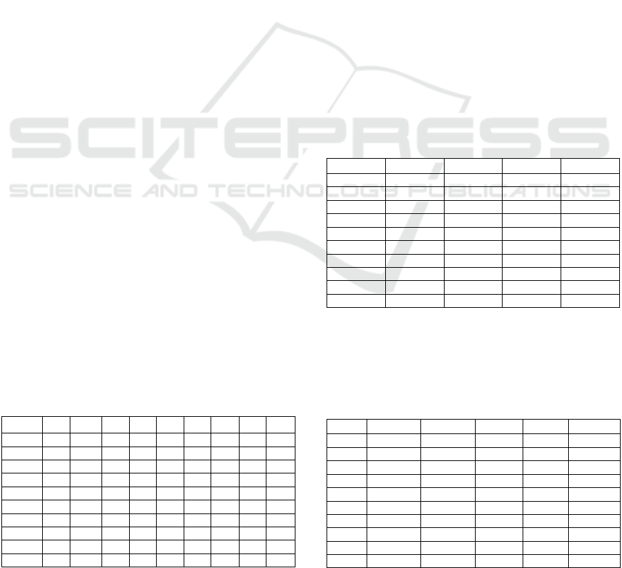
Table 3: Characteristics of the Instances.

Inst.

N M S Q L







1 20 40 10 3 4 2 1 2 0.5

2 20 70 15 4 5 3 0.5 3 1

3 20 100 20 5 6 4 0.2 4 2

4 30 50 10 3 4 2 1 2 0.5

5 30 80 20 4 6 3 0.5 3 1

6 30 120 30 5 8 4 0.2 4 2

7 40 100 20 4 5 2 1 3 1

8 40 200 40 6 10 4 0.5 4 2

9 50 150 20 4 5 2 1 3 1

10 50 300 40 6 10 4 0.5 4 2

Outputs. For every instance:

 We apply the CPLEX12 library (Table 4) to the

general PV_Prod_VRP MILP model, with 30.S

scheduled trips (Card() = 30.S). Then we get (in

less than 1 CPU h), a lower bound LB_G, an upper

bound UB_G, CPU time T_G, and the value Relax

of the rational relaxation at the root.

 We solve (Table 5) the Elementary_Trip ILP, with

 = A

Mean

/2, while using the branch and cut

algorithm of Section 3.2.2 We get lower and upper

bounds LB_S1 and UB_S1, CPU time T_S1 and

the number C_S1 of SNS cuts generated during

the process. We also provide the upper bound

UB_W obtained without the SNS constraints.

 We apply (Table 6) the global VRP_Surrogate

resolution scheme while relying on the pricing

mechanism and while setting  = A

Mean

/2 and Q

i,n

= Q

Stand

i,n

for any i, n. We denote by W_Price

resulting PV_Prod_VRP value. We do the same

(Table 6) with 8 combinations (, 



, 



 and

denote by W_Price_8 resulting value.

 We apply (Table 6) the global VRP_Surrogate

resolution scheme while relying on machine

learning and denote by W_ML related value.

Those results may be summarized as follows:

Table 4: Behavior of the PV_Prod_VRP MILP model.

Inst. LB_G UB_G T_G Relax

1 735.3 735.3 628.4 344.5

2 951.3 951.3 265.3 312.0

3 709.2 999.2 159.7 413.5

4 322.1 508.2 3600 208.7

5 969.0 969.0 1819.3 611.7

6 1153.4 1486.3 3600 764.5

7 1972.7 3065.5 3600 1652.3

8 3386.9 4211.8 3600 3008.2

9 4923.0 9594.3 3600 4021.2

10 5956.6 8560.3 3600 5365.4

Comments: As expected, the global ILP model is in

trouble, even on small instances. Still, further results

(Table 7) will make appear that, at least for small M,

upper bound UB_G looks close to optimality.

Table 5: Behavior of the Elementary Trip Branch/Cut.

Inst. LB_S1 UB_S1 T_S1 C_S1 UB_W

1 884.4 884.4 1622.5 28 884.4

2 1435.3 1488.3 1 h 67 1522.5

3 1005.9 1202.9 1 h 79 1325.0

4 774.6 774.6 1254.8 503 880.3

5 1516.2 1654.2 1 h 468 1816.2

6 1886.3 1986.3 1 h 1435 2187.0

7 3891.7 4491.7 1 h 2960 4702.8

8 5020.3 5520.3 1 h 4121 Fail

9 12023.6 14077.2 1 h 4689 Fail

10 14773.0 17773.9 1 h 2867 Fail

Synchronizing Vehicle Routing and Photo-Voltaic Production

133

Comments: Strong no_sub_tour constraints

significantly increase our ability to manage the

Elementary_Trip problem through branch and cut.

Notice that, since the Elementary_Trip model tends

to overestimate the energy purchase value, values

UB_S1 are significantly larger than values UB_G

obtained in Table 4.

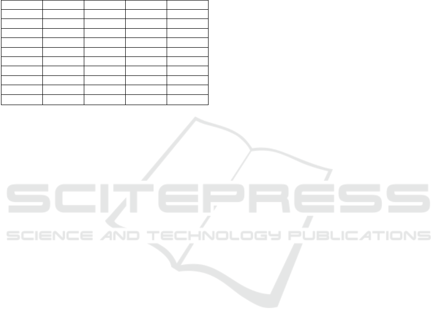
Table 6: Behavior of the Surrogate Components.

Inst. UB_G W_Price W_Price8 W_ML

1 735.3 735.3 735.3 740.8

2 951.3 966.8 951.3 980.6

3 999.2 1010.3 995.0 1030.0

4 508.2 512.6.2 504.3 508.2

5 969.0 986.5 972.6 1040.2

6 1486.3 1487.0 1487.0 1512.5

7 3065.5 3025.7 3003.5 3197.3

8 4211.8 4225.8 4200.6 4354.6

9 9594.3 9397.7 9365.9 9456.1

10 8560.3 8508.9 8475.1

Comments: Solving PV_Prod_VRP while relying on

the parametric pricing mechanism often behaves

better than the PV_Prod_VRP MILP. As for the the

machine learning oriented approach, the gap between

our best PV_Prod_VRP value and W_ML_ILP is in

average around 4%, with a peak at 7%.

5 CONCLUSIONS

We dealt here with synchronization between

consumption and production. We shortcut the

production sub-problem and replaced it by a

parametric surrogate sub-problem. But since in true

life solar energy production forecasting involves a

uncertainty, going further with machine learning

could help us in managing related risk of failure.

ACKNOWLEDGEMENTS

We thank both Labex IMOBS3 and PGMO program

for funding this research.

REFERENCES

Adulyasak Y., Cordeau J.F., Jans R. (2015).The production

routing problem: formulations and solution algorithms.

Computers & Operations Research, 55 , p 141-152.

Albrecht A., Pudney P. (2013). Pickup and delivery with a

solar-recharged vehicle. Ph.D. thesis Australian Society

for Operations Research .

Bendali F., Mole Kamga E., Mailfert J., Quilliot A.,

Toussaint H. (2021): Synchronizing Energy Production

and Routing; RAIRO-OR, 55 (4), pp. 2141-2163.

Caprara A., Carvalho M., Lodi A., Woeinger G.J (2014). A

study on the bilevel knapsack problem; SIAM Journal

on Optimization 24 (2), p 823-838.

Balbiyad S. (2019. Collective self consumption: computing

the optimal energy distribution coefficients under local

energy management; Report ENSTA/EDF OSIRIS.

Chen L., Zhang G. (2013). Approximation algorithms for a

bi-level Knapsack problem; TCS 497, p 1-12.

Colson B., Marcotte P., Savard G. (2005). Bi-level

programming: A survey; 4OR Vol 3 (2), p 87-107.

Deb S., Tammi K., Kalita K., Mahanta P. (2018). Impact of

electric vehicle charging station load on distribution

network; Energies 11 (1), p 178-185.

Dempe S., Kalashnikov V., Perez-Valdez G., Kalashikova

N. (2015).:Bi-level Programming Theory, Springer.

Erdelic T., Caric T. (2019). A survey on the electric vehicle

routing problem: Variants and solutions. Journal of

Advanced Transportation.

Grimes S., Varghese O., Ranjan S. (2008). Light, water,

hydrogen: The solar generation of hydrogen by water

photoelectrolysis. Springer-Verlag US.

Irani S., Pruhs K. (2003). Algorithmic problems in power

management. SIGACT News, 36, 2, p 63-76.

Kleinert T., Labbé M., I.jubic I., Schmidt M. (2021). A

survey on MILP in bilevel optimization. EURO Journal

on Computational Optimization 9, 21 p.

Koc C., Jabali O., Mendoza J., G.Laporte G. (2019). The

electric vehicle routing problem with shared charging

stations. ITOR, 26 , p 1211-1243.

Krzyszton M. (2018). Adapative supervison: method of

reinforcement learning fault elimination by application

of supervised learning. Proc. FEDCSIS AI, p 139-149.

Luthander R., Widen J., Nilsson D., Palm J. (2015).

Photovoltaic self-consumption in buildings: A review;

Applied Energy 142, p 80-94.

Smarter Together (2016). Reports on collective self-

consumption of photo-voltaic; Smarter Together.

Trotta M., Archetti C., Feillet D., Quilliot A. (2022). A

pickup and delivery problem with a fleet of electric

vehicles and a local energy production unit; Proc.

Triennial Symposium TRISTAN), 6 pages.

Wojtuziak G., Warden T., Herzog O. (2012). Machine

learning in agent based stochastic simulation;

Computer and Mathematics with App. 64, p 3658-3665.

ICORES 2023 - 12th International Conference on Operations Research and Enterprise Systems

134