Railway Switch Classiﬁcation Using Deep Neural Networks

Andrei-Robert Alexandrescu

, Alexandru Manole and Laura Dios¸an

Department of Computer Science, Babes¸-Bolyai University, 1, M. Kogalniceanu Street, Cluj-Napoca, Romania

Keywords:

Machine Learning, Deep Learning, Image Classiﬁcation, Railway Switches.

Abstract:

Railway switches represent the mechanism which slightly adjusts the rail blades at the intersection of two rail

tracks in order to allow trains to exchange their routes. Ensuring that the switches are correctly set represents

a critical task. If switches are not correctly set, they may cause delays in train schedules or even loss of lives.

In this paper we propose an approach for classifying switches using various deep learning architectures with

a small number of parameters. We exploit various input modalities including: grayscale images, black and

white binary masks and a concatenated representation consisting of both. The experiments are conducted on

RailSem19, the most comprehensive dataset for the task of switch classiﬁcation, using both ﬁne-tuned models

and models trained from scratch. The switch bounding boxes from the dataset are pre-processed by introducing

three hyper-parameters over the boxes, improving the models performance. We manage to achieve an overall

accuracy of up to 96% in a ternary multi-class classiﬁcation setting where our model is able to distinguish

between images containing left, right or no switches at all. The results for the left and right switch classes are

compared with two other existing approaches from the literature. We obtain competitive results using deep

neural networks with considerably fewer learnable parameters than the ones from the literature.

1 INTRODUCTION

Railway transport represents one of the most efﬁcient

ways of transporting, both people and cargo, from

one place to another (Growitsch and Wetzel, 2009).

The ﬁrst train routes were used for industrial purposes

consisting initially of a small number of stations. As

more companies considered railway transport to be a

feasible way of transporting cargo and people, more

stations were built to support the growing infrastruc-

ture. This increase led to a higher demand for building

routes between stations.

In order to optimize the train trafﬁc, switches were

introduced. Train track switches represent a break-

through mechanism which allows freight cars to ex-

change tracks and change routes by means of a set of

moving rails named blades. Generally, the engineer

driving the train is responsible for acting the switch

when the train is approaching it.

In the last decades, even though many advance-

ments were made in scene understanding for au-

tonomous driving, one problem has received a low

amount of attention: autonomous trains. These trains

should not require any human intervention for the

driving process.

https://orcid.org/0000-0003-4890-7819

https://orcid.org/0000-0002-6339-1622

At ﬁrst glance, the problem of smart (or au-

tonomous) trains appears to be easier to solve than the

smart car’s problem. Trains have a restricted space of

movement, being constrained by the rails they move

on. However, switching tracks represents a more cru-

cial process than switching car lanes when changing

routes. Trains are allowed to switch tracks only at cer-

tain locations where a switch is present. A missed or

wrong track exchange would not only delay the train,

but it might also cause interference with other trains,

which may ultimately lead to fatal events. More-

over, the problem of railway segmentation faces more

difﬁcult scenes with many different elements such

as ground embeddings, weed coverage and railroad

crossings.

This paper aims to provide answers to the follow-

ing research questions:

1. How reliable are the proposed methods for switch

classiﬁcation given a dynamic environment (i.e.

the camera on the train)?

2. How can we surpass the current state-of-the-art

for the switch classiﬁcation problem?

In this respect, we perform a set of experiments

for switch classiﬁcation on various conﬁgurations us-

ing the most comprehensive dataset from the railway

scene available at the moment.

We aim to obtain competitive results by using

Alexandrescu, A., Manole, A. and Dios

an, L.

Railway Switch Classiﬁcation Using Deep Neural Networks.

DOI: 10.5220/0011611600003417

In Proceedings of the 18th International Joint Conference on Computer Vision, Imaging and Computer Graphics Theory and Applications (VISIGRAPP 2023) - Volume 4: VISAPP, pages

769-776

ISBN: 978-989-758-634-7; ISSN: 2184-4321

 2023 by SCITEPRESS – Science and Technology Publications, Lda. Under CC license (CC BY-NC-ND 4.0)

769

deep neural networks with fewer parameters than ex-

isting solutions from the literature. The solutions

we have found in the literature use networks such as

DenseNet161 (Huang et al., 2017) with around 20M

parameters or ResNet50 (He et al., 2016) with over

23M learnable parameters. Our experiments show

that high performance can be obtained using networks

with fewer parameters which would be faster in a dy-

namic environment such as the video camera on the

train. Both ﬁne-tuned and trained from scratch mod-

els are used.

We also perform a pre-processing on the switch

images by considering more context around the

switches and eliminating some of them from the

dataset based on a few criteria. For this, three hyper-

parameters are introduced, namely α, β and γ whose

values are found empirically.

The rest of the paper is structured as follows. Sec-

tion 2 describes the existing approaches for switch

classiﬁcation and our approach is presented in Sec-

tion 3. In Section 4 we present the obtained results

and an analysis of the results. Future considerations

are mentioned in Section 5. Conclusions and a brief

overview of the paper are given in Section 6.

2 RELATED WORK

At the moment, there are not many proposed solutions

for switch classiﬁcation, nor are there many datasets

available for testing and validating this task.

Karak

ose et al. have attempted to solve the switch

classiﬁcation task by detecting crossings on the rail-

way line (Karak

ose et al., 2016). They have used

only an image-processing approach. Their pipeline

features the Canny edge detector (Canny, 1986) and

the Hough transform (Duda and Hart, 1972) in order

to ﬁnd points of intersection. Based on their posi-

tions, the switches are classiﬁed as belonging to one

of the following classes: Single left switch, Single

right switch, Symmetric switch, Compound switch,

Cross-switch or Crossover. They have obtained the

best results, between 80% and 90% success rate on

the ﬁrst two classes. The downside of this work is

that less than 30 images were used to test the model

which might be biased towards easy-to-classify im-

ages. These images were taken from a camera in-

stalled on a train located in various testing environ-

ments.

Zendel et al. have constructed a public dataset for

semantic scene understanding for trains and trams,

called RailSem19. They have used deep learn-

ing methods for solving the semantic segmenta-

tion task (Zendel et al., 2019). They experimented

with the FRRN architecture (Full-Resolution Resid-

ual Network) (Pohlen et al., 2017), pre-trained on the

Cityscapes dataset (Cordts et al., 2016) and ﬁne-tuned

using 4000 training images selected randomly from

the RailSem19 dataset. This architecture consisted of

an end-to-end model that combined feature extraction

and semantic segmentation based on the ResNet50

backbone (He et al., 2016) while preserving the full-

resolution of the input image on a separate stream.

The FRRN architecture comes in two ﬂavours:

FRRN A and FRRN B which differ from each other in

terms of the input image size: FRRN A processes im-

ages of 256 × 512 pixels, while FRRN B processes

images of 512 × 1024 pixels. Pohlen et al. have

shown that FRRN B performs better than FRRN A

since it has a larger receptive ﬁeld. Zendel et al.

have used the FRRN B version with an input size of

512×512. For the image classiﬁcation task, they have

obtained an accuracy of 53.7% for Switch-Left and

62.9% for Switch-Right using the Densenet161 archi-

tecture (Huang et al., 2017) pre-trained on ImageNet

(Russakovsky et al., 2015). These values were ob-

tained from a multi-class classiﬁcation in which other

classes were considered as well. They also experi-

mented with a one-vs-all classiﬁcation task in which

they obtained outstanding results of up to 90% ac-

curacy for the left and right switch classes. When

training on only two classes, namely Switch-Left and

Switch-Right, they report an accuracy of 67% after 20

epochs of training.

Jahan et al. also tackled the switch classiﬁcation

and detection task using deep neural networks (Jahan

et al., 2021). They have considered a one-stage ob-

ject detector called RetinaNet (Lin et al., 2017) pre-

trained on the Microsoft COCO dataset (Lin et al.,

2014). Besides training on RailSem19 (Zendel et al.,

2019), a custom private dataset named DLR is used

with 2500 instances of switches: 1272 left and 1218

right. For the classiﬁcation task, they have classi-

ﬁed left and right switches with a precision of 0.87,

0.93, recall of 0.94, 0.86 and F1-score of 0.90, 0.89

for the Switch-Left and Switch-Right classes respec-

tively. The results obtained by these researchers on

their custom dataset appear to be the current state-of-

the-art for switch classiﬁcation and detection.

At the moment, the RailSem19 dataset con-

structed by Zendel et al. is the largest publicly avail-

able dataset containing annotated images taken from

the egocentric perspective of trains. For this reason

we extensively experiment with it in this article.

VISAPP 2023 - 18th International Conference on Computer Vision Theory and Applications

770

3 OUR APPROACH

The problem of switch detection can be formulated

as an object detection task structured into two steps.

The ﬁrst step is to ﬁnd the regions of interest where

switches might be present. This can be done through

semantic segmentation (Alexandrescu and Manole,

2022). The second step is to crop the identiﬁed re-

gions and classify them.

In this paper, we describe our approach only for

the second step of this method. Unlike the state-of-

the-art, we will use the semantic segmentation masks

in our classiﬁcation process in some representations.

The masks are considered to be correctly segmented.

3.1 Switch Classiﬁcation Process

In our approach, the switch classiﬁcation step tries

to classify images of switches using different well-

known deep learning architectures: VGG (Simonyan

and Zisserman, 2015), ResNet (He et al., 2016) and

MobileNet-V2 (Sandler et al., 2018). We have also

considered a custom simple architecture containing

one single convolution operation. By using this sim-

ple architecture, our goal was to understand whether

shallower networks would beneﬁt learning.

In the following, we describe the formalism used

for our problem, the selected architectures and the

used dataset.

3.2 Formalism

A two-dimensional image can be perceived as a bidi-

mensional matrix with n rows and m columns. Its

topology is expressed and denoted by D = {1, ..., n}×

{1, ..., m}. We deﬁne img : D → E, where E may have

one of the following forms based on the image type:

• grayscale image: E = {0, ..., 255};

• RGB image: E = {0, ..., 255}

;

• binary image: E = {0, 1}.

Therefore, img(i, j) = e, where e ∈ E, i ∈

{1, ..., n}, j ∈ {1, ..., m}, (i, j) is a coordinate of the

image, and e is its value.

Similarly, the classiﬁcation model considered in

this paper may be expressed as an algorithm which

has as input an image img : D → E and as output a

label lbl ∈ {0, ...,C − 1} where C is the number of

possible classes. For our classiﬁcation problem, three

classes are considered: Switch-Left, Switch-Right and

None. A bounding box is characterized by four prop-

erties: x, y, w, h where x and y are its top-left coordi-

nates and w and h characterize its size, (x, y) ∈ D, w ∈

{1, ..., m}, h ∈ {1, ..., n}.

3.3 Architectures

The architectures we have used for switch classiﬁca-

tion are SNet, ResNet-18 (He et al., 2016), VGG-11

(Simonyan and Zisserman, 2015) and MobileNet-V2

(Sandler et al., 2018).

SNet features one single convolutional layer with

2 ﬁlters of size 5×5 and a stride of 3×1. The convo-

lutional layer has 7355 parameters for images of size

64×64, therefore it is followed by a linear layer that

maps 2400 features to 3 output nodes, one for each

class. In order to add a slight regularization effect,

two dropout layers were introduced with probabilities

70% and 50% respectively after the ReLU activation

function (Agarap, 2018) of the convolutional layer.

The VGG (Visual Geometry Group) architecture,

inspired by AlexNet (Krizhevsky et al., 2012), was

used for large-scale image recognition (Simonyan and

Zisserman, 2015). It consists of multiple versions de-

pending on the depth of the network: from 11 to 19

layers which at the time was considered very deep. It

brings only a small increase in the performance of the

model, however it requires more parameters.

One issue of the VGG was that the gradient ﬂow

was affected by a large number of layers, thus leading

to a slower learning process. It was also believed that

such networks were more prone to overﬁtting, mean-

ing that they would fail to generalize the learned rep-

resentations from the training dataset on new, unseen

samples. That claim was proved to be false in (He

et al., 2016).

In order to ﬁx the issues introduced by VGG,

Residual Neural Networks, also named ResNets, were

introduced (He et al., 2016). The authors observed

that very deep neural networks were not affected by

an overﬁtting problem, however they were harder to

be optimized. To provide a solution to this, residual

connections were added between layers that would

copy the learned features from the shallower part to

the deeper part of the network.

The ResNet-18 architecture used in this paper has

only 11M parameters; it is smaller than ResNet-50

with more than 23M learnable parameters or other

larger variants.

The previously described networks consist of a

large number of parameters which might not be suit-

able for smaller, memory-constrained devices. There-

fore, a class of neural networks was introduced, called

MobileNets (Howard et al., 2017), which replaced the

classic convolutional operation with Depthwise sepa-

rable convolutions that consist of a depthwise con-

volution and a pointwise convolution. This split de-

creases the number of computations signiﬁcantly.

The ﬁrst version of MobileNets (Howard et al.,

Railway Switch Classiﬁcation Using Deep Neural Networks

771

2017) had 4.2 million parameters. Newer versions

were introduced to decrease the number of parame-

ters and computations even more. The second version

of MobileNets (Sandler et al., 2018) has only 3.4 mil-

lion parameters.

In order to provide an answer to our ﬁrst re-

search question and deploy this method of classify-

ing switches in a dynamic environment, we have con-

sidered deep neural network architectures with a rela-

tively small number of parameters. This does not only

allow for faster training and testing, but it also leads to

small inference times when used in combination with

cameras placed on trains in the wild.

3.4 Dataset

For our experiments, we have used the RailSem19

dataset (Zendel et al., 2019) which is presently the

most comprehensive dataset from the rails domain,

used to train the models that solve the switch classiﬁ-

cation task. It is comprised of 8500 images taken from

the ego-view of the train. The images are taken from

38 countries in varying weather and lighting condi-

tions. The samples contain both ground-truth masks

(for the rails segmentation process) and bounding

boxes for the switches, classiﬁed with either switch-

left or switch-right annotations, among other classes

which are not relevant for our problem.

According to Zendel et al., there should be 1965

and 2083 bounding boxes for classes switch-left and

switch-right respectively. After closer examination of

the data, only 1963 bounding boxes for switch-left and

2080 bounding boxes for switch-right were counted.

Despite this small inconsistency, the number of sam-

ples for each class is balanced enough for us not to

make any weight adjustments to the loss function.

The bounding boxes for the switches provided in

the dataset are constrained to a small view of the

rail track, and sometimes they do not contain the full

blades required for the switch exchange. In order to

ﬁx this issue, we have considered multiple scales of

the images in a similar fashion to what has been at-

tempted in (Zendel et al., 2019). We use a hyper-

parameter α in order to retrieve the switch bounding

box as well as the area around it. If α > 1, then the

bounding box is extracted together with a padding

which is decided by α and the size of the original

bounding box. The coordinates of these boxes are

computed as in Equation 1:

′

= w ∗ α

′

= h ∗ α

′

= x − (w

′

− w)

′

= y − (h

′

− h)

(1)

where w, h, x, y are the coordinates of the original

bounding box and w

′

, h

′

, x

′

, y

′

are the coordinates of

the upscaled bounding box. After the padding is

applied, the resulting bounding boxes are resized to

224×224 pixels such that the data samples are con-

sistent. Figure 1 illustrates how various values for α

inﬂuence the original bounding box.

We have introduced another hyper-parameter to

eliminate the bounding boxes that are smaller in width

or height than β pixels. After some experiments,

the chosen value for β is set to be 30. Thus, all

bounding boxes with width or height less than 30 are

not considered. This step led to the removal of 980

switches from the dataset, comparatively to (Zendel

et al., 2019) where 1049 switches were removed by

using a β = 28.

The last hyper-parameter used is γ for eliminating

the images that have too many pixels of the rails class.

This issue may occur for small bounding boxes, how-

ever it was observed that even for large values of β,

there still were some resulting bounding boxes with

too many positive pixels, increasing the difﬁculty of

the task for the classiﬁer. In order to ﬁx this, the γ

hyper-parameter is used and set to 0.75. This means

that bounding boxes with more than 75% rail pixels

are eliminated.

3.5 Switch Classiﬁcation Approach

We consider switch classiﬁcation as an image classi-

ﬁcation task with three classes: Switch-Left, Switch-

Right and None.

We have performed a comprehensive set of ex-

periments using different images of switches of size

224 ×224 pixels. We have used grayscale images, se-

mantic segmentation mask images, augmented mask

images, and a combined representation of grayscale

and mask images. The ﬁrst two types are self-

explanatory. The image augmentations used were

shifting with a factor of 0.07 on X and 0.05 on

Y axes, and rotating them with at most 10°. The

combined representation is depicted in Figure 2.

It implies concatenating channel-wise (depth-wise)

the single-channel grayscale image together with the

mask which also has a single channel, leading to a

two-channel volume, and the same dimensions as the

original images. By concatenating the two possible

switch representations, the neural networks beneﬁt

from more context when learning to model the data.

The used SNet architecture has the least number

of parameters: 97835, while ResNet-18 and VGG-

11 have 11 and 34 million parameters respectively.

The MobileNet-V2 architecture has only 3.4 param-

eters. A batch size of 32 was chosen with an 80:20

VISAPP 2023 - 18th International Conference on Computer Vision Theory and Applications

772

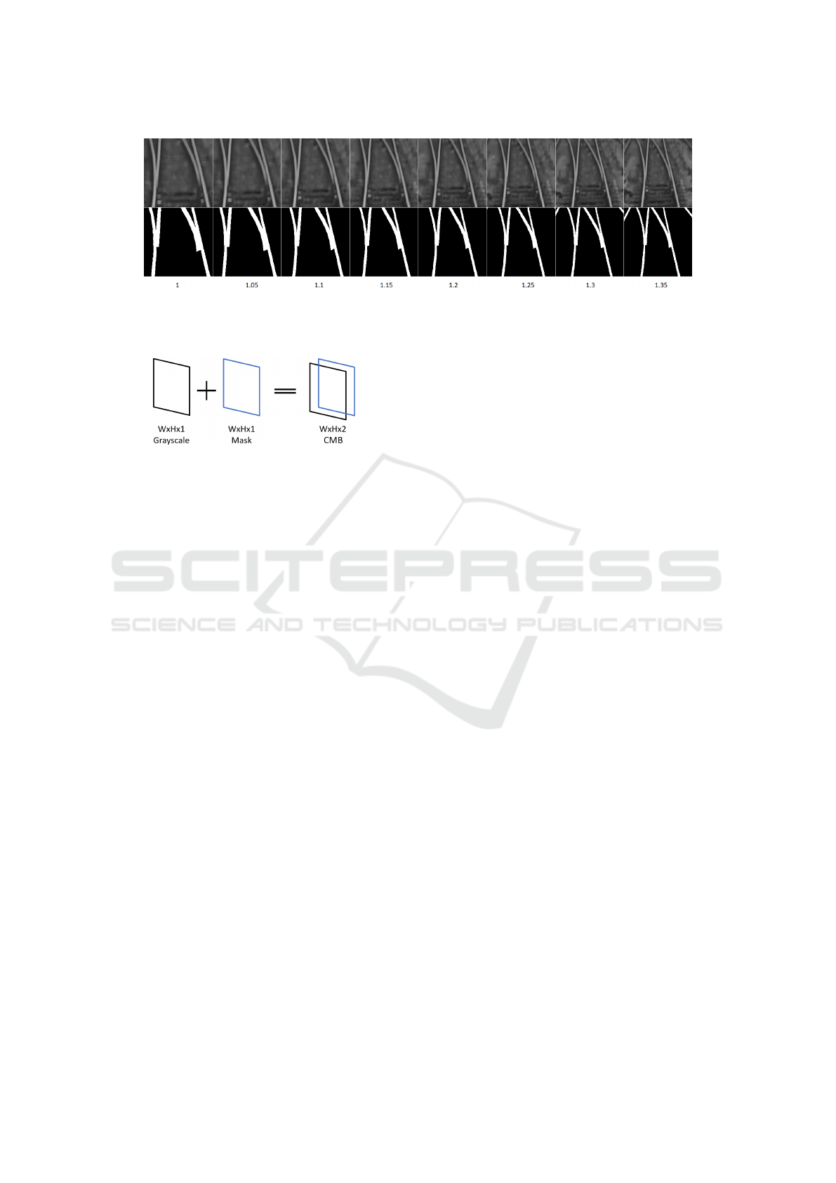
Figure 1: Comparison between bounding boxes for switches based on various α values. Each column corresponds to a

different α value. The ﬁrst row contains the grayscale image of a switch. The second row contains the segmentation mask for

the image.

Figure 2: Channel-wise concatenation of grayscale and

mask images to obtain the combined (CMB) representation.

data split between training and validation samples. In

order to gain a sense of the overall performance of

the trained models, 8 different seeds were considered

for each test. Adam (Kingma and Ba, 2015) with ini-

tial learning rate of 1e

−4

was used for optimization.

Two Nvidia Tesla K40X GPUs were used for train-

ing. The experiments were written in Python using

the PyTorch library. The image augmentations were

applied with a probability of 50%.

One of the purposes of these experiments was to

identify the best α hyper-parameter as well as to de-

termine whether the augmentations improve the per-

formance of the model on unseen data. Since the

masks for each switch were available, we have exper-

imented with them to see whether our results obtained

on the masks are better than the ones on the images.

4 RESULTS

This section details the results of our approach for the

switch classiﬁcation task. We focus on a speciﬁc set

of metrics and provide insight into the obtained re-

sults. The research questions are answered at the end.

4.1 Metrics

In order to evaluate the obtained results, we have used

the following metrics: Accuracy, Precision, and Re-

call, as these are ubiquitous metrics for image classi-

ﬁcation tasks.

We have computed the overall Accuracy, Pre-

cision, and Recall metrics for each of the classes:

Switch-Left, None and Switch-Right. Since the con-

sidered dataset was balanced and the number of in-

stances for each class is almost identical, the accuracy

metric is meaningful. The precision and recall metrics

were computed as well in order to offer a robust view

over the performance of the models.

Experiments were conducted using various values

for the α hyper-parameter taken from the set {1, 1.2,

1.35} and ﬁxed values for β = 30 and γ = 0.75. Out of

all results, only the most meaningful ones are present

in Table 1 for each architecture.

The Conﬁg column from the table has the follow-

ing structure: architecture-alpha-type. The type can

be: omitted for grayscale images, AM for augmenta-

tions on the masks and CMB for the combined repre-

sentation. The type parameter can also take the value

PT which means that the architecture was pre-trained

on ImageNet (Russakovsky et al., 2015). The alpha

parameter can take values from the set {1.2, 1.35,

ALL} where ALL implies training on all α values.

The ﬁrst six rows present the best conﬁguration

found for each of the considered networks conﬁgu-

rations. The last two rows contain the results ob-

tained by other selected works that use the RailSem19

dataset on two classes: Switch-Left and Switch-Right.

Zendel et al. reach an accuracy score of 67% by ex-

panding the crops and ignoring samples with less than

28x28 pixels. The ﬁnal row presents the results ob-

tained by Jahan et al., focusing on the precision and

recall scores.

We observe that training on larger α values yields

better results compared to an α = 1 which resembles

the original image crops. As expected, training and

validating on all α values at the same time increases

the results signiﬁcantly.

In Figure 3 the results are showcased in a for-

mat easy to visualize. Similar notations to Table 1

are used. In addition, A denotes the results for aug-

mented grayscale images. These visualizations show

Railway Switch Classiﬁcation Using Deep Neural Networks

773

Table 1: Comparison between our best results for each model and the literature’s results for the switch classiﬁcation. The

bottom results are copied from the compared literature articles. They do not experiment on three classes as we do.

Conﬁg Accuracy Precision-Left Recall-Left Precision-None Recall-None Precision-Right Recall-Right

SNet-1.35-AM 77.17 ± 3.51 70.53 ± 4.11 71.03 ± 2.30 90.11 ± 6.74 90.09 ± 4.27 71.13 ± 2.49 70.77 ± 4.51

ResNet-1.35-CMB 84.12 ± 1.42 81.74 ± 4.89 78.59 ± 4.35 94.24 ± 2.63 92.53 ± 2.60 77.32 ± 2.83 81.58 ± 5.17

VGG-1.2-AM 88.52 ± 1.51 81.48 ± 2.39 83.76 ± 4.94 99.67 ± 0.48 99.59 ± 0.78 83.96 ± 5.04 81.88 ± 2.74

Mobile-1.35-CMB 85.65 ± 0.62 82.18 ± 2.82 82.03 ± 2.60 94.18 ± 1.84 93.10 ± 2.32 80.59 ± 2.25 81.49 ± 4.43

Mobile-ALL 89.94 ± 0.61 89.55 ± 1.61 83.80 ± 2.16 93.30 ± 0.77 98.39 ± 0.81 86.87 ± 1.83 87.47 ± 1.85

Mobile-ALL-PT 95.93 ± 0.20 94.54 ± 1.16 93.09 ± 1.38 99.94 ± 0.11 100 ± 0.00 93.34 ± 1.11 94.65 ± 1.22

DenseNet161

67.0 - - - - - -

(Zendel et al., 2019)

ResNet-50

- 93.0 86.0 - - 87.0 94.0

(Jahan et al., 2021)

the overall accuracy scores for every conﬁguration

considered on every architecture, besides the conﬁg-

uration using all α values at the same time. Figure 4

presents results solely on the MobileNet-V2 architec-

ture trained and validated on all α values considered

(1, 1.2, 1.35). Each color corresponds to each con-

ﬁguration: red for Normal, yellow for Mask and blue

for CMB. Normal stands for grayscale images of the

switches, Mask means black and white images, while

CMB represents the combined version discussed pre-

viously in Subsection 3.5. The three bars ending

with PT represent the pre-trained version of the archi-

tecture which, as expected, leads to higher accuracy

scores.

4.2 Analysis

For the SNet architecture, it may be observed that

there is an increase in the accuracy scores when aug-

mentations are used on the ground-truth masks. Aug-

mentations were expected to boost the scores, how-

ever there was nothing to hint towards the effective-

ness of masks in solving this task.

Another observation is that as α is increased, the

values of the metrics increase as well. This was ex-

pected since a higher α value implies that bounding

boxes contain more information. This leads one to

believe that the context, i.e. details around the switch,

is indeed important when classifying switches.

Another conclusion that was expected when train-

ing is that using various values for α at the same time

leads to better results. This can be attributed to the

fact that using a larger set of images for training al-

lows the architectures to better model the features that

distinguish switches from other objects and from dif-

ferent classes of switches.

Compared to Zendel et al., our results show

greater accuracy values. On the binary task of distin-

guishing between Switch-Left and Switch-Right, they

obtained an average accuracy of 67% after 20 epochs.

We have trained for 100 epochs on three classes by in-

troducing the None class and have obtained accuracy

scores of up to 96%.

Most of the training attempts showed an overﬁt-

ting behavior which was slightly diminished by the

usage of augmentations, yet still present. For all ar-

chitectures, depending on the value of α used, an in-

crease in performance is registered when augmenta-

tions and ground-truth masks are used. The SNet ar-

chitecture becomes dramatically better with the usage

of these enhancements.

Comparing the architectures between each other,

we observe that the best results are registered by the

MobileNet-V2 model, classifying correctly almost all

None-labelled images and classifying the two classes

of interest with an accuracy of 95%.

Given the results from Table 1, we observe that

if we train on a conﬁguration using a single value

for α, the VGG-11 architecture leads to the best re-

sults. This is numerically true, however, for almost all

conﬁgurations, as shown in Figure 3, the MobileNet-

V2 architecture led to the highest accuracy scores.

Besides leading to the best results, MobileNet-V2

also has the fewest learnable parameters compared to

VGG-11 or ResNet-18. SNet is not considered for

this comparison since it is a single convolutional layer

architecture used mainly to test the pipeline.

Comparing our results to the state-of-the-art re-

sults reported by Jahan et al., we have obtained lower

precision and recall values when using models trained

from scratch. Despite this, when we perform transfer

learning on pre-trained models, our scores increase,

as it can be seen in Figure 4.

Their precision and recall values are unbalanced,

having a higher precision for left switches and a

higher recall for right switches. Our precision and

recall metrics show more stable results. This being

said, a comparison between the two approaches is im-

possible to be made as the models were trained on

different datasets. They do not consider the combined

input representation we experiment with.

The architectures we have considered for the

switch classiﬁcation task require considerably less

parameters than the competition. While Zendel et

al. use a DenseNet-161 (Huang et al., 2017) with

20M learnable parameters and Jahan et al. use Reti-

VISAPP 2023 - 18th International Conference on Computer Vision Theory and Applications

774

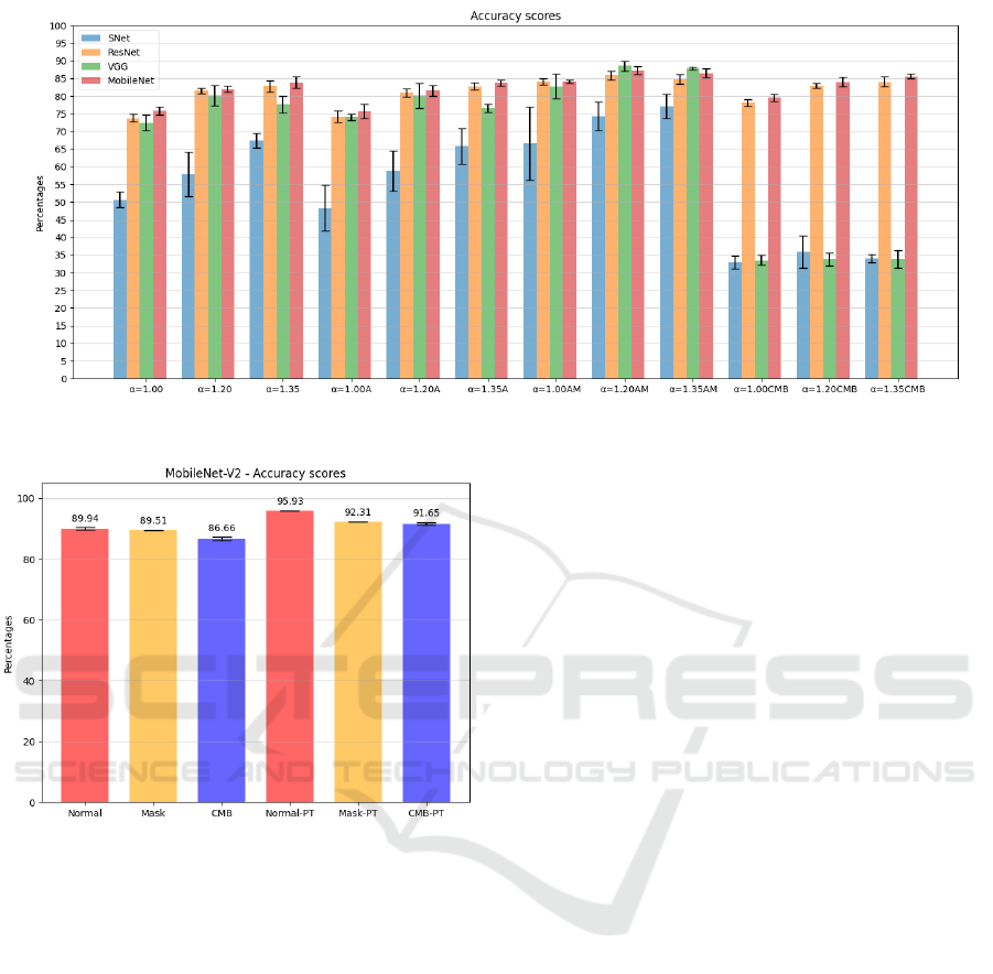
Figure 3: Comparison between architectures for each conﬁguration. Grouping made on different α values conﬁgurations.

Figure 4: Additional comparisons only for the MobileNet-

V2 architecture on all α values.

naNet (Lin et al., 2017) which consists of a ResNet50

(He et al., 2016) backbone with more than 23M pa-

rameters, ResNet-18 has only 11M parameters and

MobileNet-V2 has even less parameters with 3.4M.

From a numerical performance point of view, be-

sides SNet, all architectures lead to competitive and

reliable results on the considered metrics. Given a dy-

namic environment, the most reliable model should be

the one with the best metrics performance and small-

est inference time. The MobileNet-V2 architecture

falls into this category, having the fewest number of

parameters with 3.4M, 3 times less than ResNet-18

and 10 times less than VGG-11.

With our experiments we obtained competitive re-

sults compared to the state-of-the-art for switch clas-

siﬁcation using various architectures, each with its

perks and tweaks. We manage to obtain high preci-

sion and recall scores especially after using the pre-

trained MobileNet-V2 architecture. Note that in our

experiments we use the additional None class, thus

the comparisons are not perfect.

To provide concrete answers to the research ques-

tions from Section 1:

1. The samples used for validating our experiments

contain images of switches taken from a camera

positioned on top a moving train at various speeds.

Some of the images suffer from motion blur which

mimics real use-cases. We have not tested the

classiﬁer in a real-life scenario though, i.e. plac-

ing ourselves a camera on top of a train and ex-

tracting crops of switches from its feed. The reli-

ability can be quantiﬁed by the values of the met-

rics discussed in this section in comparison to re-

sults obtained by other authors.

2. As a result of our experiments, in order to sur-

pass the state-of-the-art results for the switch

classiﬁcation task, a pre-trained version of the

MobileNet-V2 architecture can be used and

trained on images of various sizes (various α val-

ues) from the RailSem19 dataset.

5 FUTURE CONSIDERATIONS

For future research, there are some considerations that

can be made regarding a more enhanced dataset.

The current bounding box selection process for

the switch classes Switch-Left and Switch-Right does

not follow a precise rule regarding their extraction.

Some switch crops could be observed in different po-

sitions, sometimes containing the whole mobile rail,

while other times cutting it short. This lack of consis-

tency represents one area of improvement.

Another area worth investigating is the the strat-

egy based on combining multiple modalities. Al-

Railway Switch Classiﬁcation Using Deep Neural Networks

775

though promising, this representation does not con-

siderably boost the performance of the models. More

investigations can be made in this area of multi-modal

methods. We also intend to focus on classifying

switches observed from larger distances.

6 CONCLUSIONS

In this paper we proposed an efﬁcient approach for

switch classiﬁcation using different neural networks

architectures on images taken from the perspective

of the train. The considered architectures, namely

ResNet-18, VGG-11 and MobileNet-V2, led to some

competitive results when compared to two of the few

existing approaches found to solve this task on the

considered dataset. Despite the high values of the

metrics obtained, the task of switch classiﬁcation still

remains a difﬁcult one. This paper represents a con-

siderable step forward towards solving this task.

ACKNOWLEDGEMENTS

This work was supported by two grants from Babes¸-

Bolyai University, projects numbers 6851/2021 and

18/2022.

REFERENCES

Agarap, A. F. (2018). Deep learning using rectiﬁed linear

units (relu). arXiv preprint arXiv:1803.08375.

Alexandrescu, A.-R. and Manole, A. (2022). A dynamic

approach for railway semantic segmentation. Studia

Universitatis Babes-Bolyai, Informatica, 67(1):61–

76.

Canny, J. (1986). A computational approach to edge de-

tection. IEEE Transactions on pattern analysis and

machine intelligence, 8(6):679–698.

Cordts, M., Omran, M., Ramos, S., Rehfeld, T., Enzweiler,

M., Benenson, R., Franke, U., Roth, S., and Schiele,

B. (2016). The cityscapes dataset for semantic urban

scene understanding. In Proceedings of the IEEE con-

ference on computer vision and pattern recognition,

pages 3213–3223.

Duda, R. O. and Hart, P. E. (1972). Use of the hough trans-

formation to detect lines and curves in pictures. Com-

munications of the ACM, 15(1):11–15.

Growitsch, C. and Wetzel, H. (2009). Testing for economies

of scope in european railways: an efﬁciency analysis.

Journal of Transport Economics and Policy (JTEP),

43(1):1–24.

He, K., Zhang, X., Ren, S., and Sun, J. (2016). Deep resid-

ual learning for image recognition. In Proceedings of

the IEEE conference on computer vision and pattern

recognition, pages 770–778.

Howard, A. G., Zhu, M., Chen, B., Kalenichenko, D.,

Wang, W., Weyand, T., Andreetto, M., and Adam,

H. (2017). Mobilenets: Efﬁcient convolutional neu-

ral networks for mobile vision applications. arXiv

preprint arXiv:1704.04861.

Huang, G., Liu, Z., Van Der Maaten, L., and Weinberger,

K. Q. (2017). Densely connected convolutional net-

works. In Proceedings of the IEEE conference on

computer vision and pattern recognition, pages 4700–

4708.

Jahan, K., Niemeijer, J., Kornfeld, N., and Roth, M. (2021).

Deep neural networks for railway switch detection

and classiﬁcation using onboard camera images. In

2021 IEEE Symposium Series on Computational In-

telligence (SSCI), pages 01–07. IEEE.

Karak

ose, M., Akın, E., and Yaman, O. (2016). Detection of

rail switch passages through image processing on rail-

way line and use of condition-monitoring approach.

International Conference on Advanced Technology &

Sciences.

Kingma, D. P. and Ba, J. (2015). Adam: A method for

stochastic optimization. In Bengio, Y. and LeCun,

Y., editors, 3rd International Conference on Learning

Representations, Conference Track Proceedings.

Krizhevsky, A., Sutskever, I., and Hinton, G. E. (2012). Im-

agenet classiﬁcation with deep convolutional neural

networks. Advances in neural information processing

systems, 25:1097–1105.

Lin, T.-Y., Goyal, P., Girshick, R., He, K., and Doll

ar, P.

(2017). Focal loss for dense object detection. In

Proceedings of the IEEE international conference on

computer vision, pages 2980–2988.

Lin, T.-Y., Maire, M., Belongie, S., Hays, J., Perona, P.,

Ramanan, D., Doll

ar, P., and Zitnick, C. L. (2014).

Microsoft coco: Common objects in context. In Euro-

pean conference on computer vision, pages 740–755.

Springer.

Pohlen, T., Hermans, A., Mathias, M., and Leibe, B. (2017).

Full-resolution residual networks for semantic seg-

mentation in street scenes. In Proceedings of the IEEE

Conference on Computer Vision and Pattern Recogni-

tion, pages 4151–4160.

Russakovsky, O., Deng, J., Su, H., Krause, J., Satheesh, S.,

Ma, S., Huang, Z., Karpathy, A., Khosla, A., Bern-

stein, M., et al. (2015). Imagenet large scale visual

recognition challenge. International journal of com-

puter vision, 115(3):211–252.

Sandler, M., Howard, A., Zhu, M., Zhmoginov, A., and

Chen, L.-C. (2018). Mobilenetv2: Inverted residu-

als and linear bottlenecks. In Proceedings of the IEEE

conference on computer vision and pattern recogni-

tion, pages 4510–4520.

Simonyan, K. and Zisserman, A. (2015). Very deep con-

volutional networks for large-scale image recognition.

In International Conference on Learning Representa-

tions.

Zendel, O., Murschitz, M., Zeilinger, M., Steininger, D.,

Abbasi, S., and Beleznai, C. (2019). Railsem19: A

dataset for semantic rail scene understanding. In Pro-

ceedings of the IEEE/CVF Conference on Computer

Vision and Pattern Recognition Workshops.

VISAPP 2023 - 18th International Conference on Computer Vision Theory and Applications

776

REFERENCES

Agarap, A. F. (2018). Deep learning using rectified linear