Enhancing Time Series Classiﬁcation with Self-Supervised Learning

Ali Ismail-Fawaz, Maxime Devanne, Jonathan Weber and Germain Forestier

IRIMAS, Universit

e Haute-Alsace, Mulhouse, France

Keywords:

Self Supervised, Time Series Classiﬁcation, Semi Supervised, Triplet Loss.

Abstract:

Self-Supervised Learning (SSL) is a range of Machine Learning techniques having the objective to reduce

the amount of labeled data required to train a model. In Deep Learning models, SSL is often implemented

using speciﬁc loss functions relying on pretext tasks leveraging from unlabelled data. In this paper, we explore

SSL for the speciﬁc task of Time Series Classiﬁcation (TSC). In the last few years, dozens of Deep Learning

architectures were proposed for TSC. However, they almost exclusively rely on the traditional training step

involving only labeled data in sufﬁcient numbers. In order to study the potential of SSL for TSC, we propose

the TRIplet Loss In TimE (TRILITE) which relies on an existing triplet loss mechanism and which does not

require labeled data. We explore two use cases. In the ﬁrst one, we evaluate the interest of TRILITE to boost a

supervised classiﬁer when very few labeled data are available. In the second one, we study the use of TRILITE

in the context of semi-supervised learning, when both labeled and unlabeled data are available. Experiments

performed on 85 datasets from the UCR archive reveal interesting results on some datasets in both use cases.

1 INTRODUCTION

Time Series Classiﬁcation (TSC) has been a challeng-

ing problem addressed by many researchers. While

some approaches used basic Machine Learning tech-

niques, more recently, the usage of Deep Learn-

ing models has been addressed for classiﬁcation (Is-

mail Fawaz et al., 2019; Ismail Fawaz et al., 2020),

clustering (Lafabregue et al., 2022; Anowar et al.,

2022), averaging (Terefe et al., 2020), adversarial at-

tacks (Pialla et al., 2022b), etc. This is particularly

due to the availability of more data, especially after

the release of the UCR archive (Dau et al., 2019). The

problem at hand is to ﬁnd a function that maps each

sample in the dataset to it’s corresponding label.

Trying to learn a one-to-one mapping from sam-

ples to labels can be sometimes challenging. This is

due to the lack of labeled samples a dataset includes.

Some approaches use data augmentation, (Fawaz

et al., 2018; Pialla et al., 2022a; Kavran et al., 2022)

To overcome this problem, Self-Supervised Learning

(SSL) offers a way to learn a discriminant latent space

without learning to map each sample into a label,

which is an advantage over supervised learning.

SSL is used in two main ways, either using con-

trastive loss or triplet loss. On one hand, the con-

trastive loss aims to learn how to embed a sample

and its augmented view to the same point in the latent

space. For example, it has been used on image classi-

ﬁcation (Chen et al., 2020; Grill et al., 2020) and hu-

man action recognition (Lin et al., 2020). The triplet

loss on the other hand aims to learn how to embed a

sample and its augmented representation (called pos-

itive representation) to the same point while learning

how to differ those last two from a representation of

another sample (called negative representation). The

triplet loss was introduced in (Schroff et al., 2015) for

face recognition and used for knowledge distillation

in (Liang et al., 2021; Oki et al., 2020). The dif-

ference between the two losses is the strictness. The

contrastive loss is less strict on choosing what repre-

sentations should not be close to the original, on con-

trary to the triplet loss. In other words, the contrastive

loss does not consider a negative representation, only

positive ones.

Inspired by all those applications, we are inter-

ested in adapting the SSL into the time series do-

main using the triplet loss (Schroff et al., 2015) with

our own augmentation method adapted to time se-

ries. Although in imaging we have access to large

archives such as Imagenet (Deng et al., 2009), it is

not the same in the time series domain. In addi-

tion, the problem of annotating time series datasets

is more frequent than in imaging. For instance, in

imaging, for the majority of datasets, one can use

crowd-sourcing to annotate the data samples. This

Ismail-Fawaz, A., Devanne, M., Weber, J. and Forestier, G.

Enhancing Time Series Classiﬁcation with Self-Supervised Learning.

DOI: 10.5220/0011611300003393

In Proceedings of the 15th International Conference on Agents and Artiﬁcial Intelligence (ICAART 2023) - Volume 3, pages 40-47

ISBN: 978-989-758-623-1; ISSN: 2184-433X

 2023 by SCITEPRESS – Science and Technology Publications, Lda. Under CC license (CC BY-NC-ND 4.0)

approach is not that easily suitable in the time se-

ries domain, given that most of the times, it would

be difﬁcult to differentiate between time series sam-

ples and annotate them. As a result, for time series,

usually one should refer to an expert for the annota-

tion part. To the best of our knowledge, most of the

methods that have been developed for SSL on time se-

ries evaluate their model considering fully unlabeled

data, which is usually not the case in real-world sce-

narios. In most of these work, SSL is ﬁrst applied

on the data and then a 1-Nearest Neighbor (1-NN)

strategy is employed on the output representations for

the classiﬁcation task. However, in real-world sce-

narios, due to the difﬁculty to annotate time series,

we usually are in one of these two cases: (1) only

a small annotated dataset is available or (2) a larger

dataset may be available but only a small part of it is

annotated. In both of these cases, supervised learn-

ing usually overﬁts quickly because the few amount

of annotated samples makes the dataset hard to learn

from. To overcome this limitation, SSL is one possi-

ble solution by learning representations of time series

without the labels information. The question that re-

mains is how to evaluate the self-supervised model?,

i.e, how can we know if the model learns meaningful

representation of input time series? In this paper we

propose a new SSL approach, TRIplet Loss In TimE

(TRILITE) and evaluate it for theses two cases. First,

we consider the case of having small annotated time

series datasets (Use case 1), which we tackle using

a self-supervised approach in combination of super-

vised learning, by concatenating the output represen-

tations in order to learn more features. This can be

considered as a booster for supervised models if the

SSL features are learned in a good way. Second, we

consider the case of having lager time series datasets

but still with few labeled samples (Use case 2), which

we tackle using a semi-supervised approach leverag-

ing unlabeled samples. This is to prove that SSL can

also take into account unlabeled data in order to learn

a more discriminant latent space and produce better

representations for the labeled samples.

The main contributions of this papers are:

• a new method of time series augmentation

adapted to the context of SSL.

• a new SSL approach based on the triplet loss in-

troduced by (Schroff et al., 2015). Usually other

methods use the contrasitve loss and we want to

assess the triplet loss’s contribution in SSL for

TSC.

• a new way of evaluating self-supervised model

which to the best of our knowledge was not em-

ployed before. Here we showed that with the

help of self-supervised combined with supervised

learning we can achieve better performance than

supervised learning alone on some datasets.

The rest of the paper is organized as follows: in

section 2 we introduce some related work on SSL

for time series, in section 3 we explain in details our

method, in section 4 we evaluate our self-supervised

model on the UCR archive (Dau et al., 2019) and we

ﬁnish with a conclusion in section 5.

2 RELATED WORK

2.1 Self-Supervised Learning

SSL for time series was addressed in two main ways,

using contrastive learning and triplet loss. It was ﬁrst

addressed for univariate time series in (Franceschi

et al., 2019). The authors used a triplet loss to make

the model learn how to differentiate between the la-

tent representations of an anchor time series, a posi-

tive representation of it and several negative represen-

tations. The authors used an unsupervised way to gen-

erate their triplets motivated by the problem of vari-

able length time series. While their anchor time series

is a sub-sequence of a chosen sample, the positive rep-

resentation is deﬁned as a sub-sequence of the anchor

and the negative representation as a sub-sequence of

a randomly selected sample. The advantage of their

approach is the insensitivity to variable length time

series. Its disadvantage is that it does not perturb the

positive representations, hence it facilitates the learn-

ing task. This is due to the resemblance between the

reference time series and its positive representation.

On the other hand, in (Wickstrøm et al., 2022),

the authors addressed the mixing up proposal between

two time series. They used a contrastive learning ap-

proach to predict the amount of mixing up from two

different time series in order to learn representations

in the latent space.

For each pair of input time series randomly sampled,

they create a third sample mixed up from it. This

method overcomes the lack of perturbation added to

the time series in (Franceschi et al., 2019) but to the

best of our knowledge was never tested using a triplet

loss.

Originally, in (Schroff et al., 2015), the authors

introduced the SSL world with the triplet loss which

was motivated from the Siamese network. The au-

thors applied it for face detection using positive and

negative examples of the reference image. This in-

duces into the network not only features of the ref-

erence image but also similarities and dissimilarities

with other images. This was motivated by the lack of

available samples.

Enhancing Time Series Classiﬁcation with Self-Supervised Learning

Differently, the authors of (Yang et al., 2022) pro-

posed an adaptation of SimCLR (Chen et al., 2020)

but with taking into consideration the temporal depen-

dencies between data points in time series.

In addition, some authors contribute in SSL for

Multivariate Time Series (MTS), like in (Chen et al.,

2022) where the authors constructed a channel-aware

self-supervised model using a transformer encoder for

MTS. Taking into consideration both channel-wise

and time-wise features by training two encoders, one

to ﬁnd the similarity using the contrastive loss and the

other to predict the next trend. Another contribution

was made in SSL for MTS in (Mohsenvand et al.,

2020) where the authors introduced SeqCLR which

was an adaptation of SimCLR (Chen et al., 2020).

The authors worked on SSL for electroencephalogram

classiﬁcation where they faced two problems. The

ﬁrst was the lack of data and the second was what

the type of data augmentation they should use for the

contrastive learning.

Distinctively, some work addressed the dimen-

sionality reduction problem like in (Garg, 2021). The

authors used an autoencoder where their encoder and

decoder were adapted from a LeNet (LeCun et al.,

1998) trained on both the reconstruction loss at the

output of the decoder and the triplet loss (Schroff

et al., 2015) using the triplets generated in the bot-

tleneck layer.

Moreover, the authors in (Eldele et al., 2021) sug-

gested a method based on temporal and contextual

contrastive learning using transformers. First they

suggested using two different augmentations for the

same input time series and feed them to a Siamese

network with a FCN encoder. This was followed by

a transformer to learn cross-view prediction task of

time steps while maximizing similarities between two

predictions from different views. This was to help

with the forecasting part of the model but at the same

time apply contrastive learning on the two predicted

representations.

In addition, a review (Lafabregue et al., 2022) on

deep representation learning for time series cluster-

ing sets the benchmark of clustering techniques on

the UCR archive (Dau et al., 2019). The authors var-

ied between which architecture to use, which clus-

tering loss and pretext loss to use. One of the pre-

text loss in this review was the triplet loss proposed

in (Franceschi et al., 2019). The clustering loss is ap-

plied on the latent representations.

2.2 Deep Learning Methods for Time

Series Classiﬁcation

Deep learning for TSC has been a very targeted do-

main in the past few years. In (Ismail Fawaz et al.,

2019), a comparison was made between different

architectures starting from Multi Layer Perceptron

(MLP) to end up with ResNet (Wang et al., 2017).

It was shown in (Ismail Fawaz et al., 2019) how the

use of convolution networks like Fully Convolutional

Network (FCN) (Wang et al., 2017) and residual con-

nections (ResNet) (He et al., 2016) are signiﬁcantly

better than other approaches. Some work (Mercier

et al., 2022) also analyse the explanation of con-

volution classiﬁers for time series. More recently,

the InceptionTime (Ismail Fawaz et al., 2020) model

showed a signiﬁcant difference in performance by

concatenating the output of many convolution lay-

ers with different characteristics instead of tuning on

one convolution layer. This creates several receptive

ﬁelds for the model to learn from. In addition, knowl-

edge distillation techniques (Hinton et al., 2015) have

been adapted for Time Series Classiﬁcation (Ay et al.,

2022) where the authors transfer the knowledge from

a FCN to a smaller convolution neural network.

In our case, we are interested in evaluating the

contribution of the triplet loss in the case of TSC.

Hence we chose a simple FCN architecture as a back-

bone of our TRILITE model detailed in the next sec-

tion.

3 TRIPLET LOSS IN TIME

3.1 Deﬁnitions

Before describing the model, we deﬁne some impor-

tant terms used in the rest of the paper.

Time Series. A time series is a sequential data rep-

resentation of an event changing over time in an

equally separated manner. We deﬁne a univariate time

series as X = [x

, x

, ..., x

], L being the number of

time steps of this time series. A batch X = {X}

set of N time series of length L.

Representations. An anchor time series is referred

to as re f , a positive representation of the anchor as

pos and a negative representation of the anchor as neg.

Metrics. A distance between 2 representations

d(., .) is referred to the Euclidean distance between

2 vectors.

ICAART 2023 - 15th International Conference on Agents and Artiﬁcial Intelligence

Triplet Loss

Encoder

ref

pos

neg

Figure 1: Overview of our TRILITE model.

3.2 Model

Our proposed TRILITE model is composed of three

encoders with weights shared between them. It cor-

responds to one encoder fed by the triplets generated

as it can be seen in Figure 1. In our case, the encoder

architecture is the FCN from (Wang et al., 2017) and

implemented in (Ismail Fawaz et al., 2019). However,

we remove the classiﬁcation layer as we are consider-

ing a self-supervised case. Each triplet’s sample re f ,

pos and neg are passed through the model to obtain

the latent representation re f

, pos

and neg

. These

latent representations are of size 128.

3.3 Triplet Loss

Inspired by (Schroff et al., 2015) where triplet loss

was used for face recognition, we propose to use a

similar loss for the case of time series. The triplet

loss for a given triplet is deﬁned as:

Loss = max(0, α +d(re f

, pos

)−d(re f

, neg

)). (1)

The goal of this loss is to increase the distance be-

tween the re f

and neg

but to decrease the distance

between re f

and pos

. In order to relax this mini-

mization problem, an α hyperparameter is added to

control the margin between these two distances. As a

result we can identify 3 types of triplets as shown in

Figure 2:

• Easy Triplet: The Loss = 0 because

d(re f

, pos

) + α < d(re f

, neg

)

• Hard Triplet: The neg

is closer to the re f

than

pos

, d(re f

, neg

) < d(re f

, pos

)

• Semi-Hard Triplet: The case is good

d(re f

, pos

) < d(re f

, neg

) but we got a

positive loss

We note that if α = 0, only two triplets can be de-

ﬁned, the easy triplets and the hard triplets. Using

only easy triplets would overﬁt the model and using

only the hard triplets would underﬁt the model. This

motivates the use of the hyperparameter α to create

margin α

semi-hard negatives

easy negatives

hard negatives

ref

neg

pos

Figure 2: Schema of the relaxed spaced controlled by the

margin α.

the in-between space of semi-hard triplets. In addi-

tion, in 1, the max operation in the loss aims to trans-

form the problem into a convex one.

3.4 Triplet Generation

In order to generate triplets i.e.pos and neg generated

from re f , two main approaches have been proposed.

In (Wickstrøm et al., 2022) a mixing up strategy is

employed. In (Franceschi et al., 2019) a masking ap-

proach is used. In this work, our triplet generation ap-

proach consists of combining both methods into one,

as detailed in Algorithm 1. First, a pos is created us-

ing a weighted sum of three time series, the re f in-

cluded. For the neg, the same process is applied ex-

cept that the re f is not included in the weighted sum.

We limit the number of mixed up samples to three to

ensure that each sample can contribute in a signiﬁcant

manner. This generation process is summarized in the

following equations:

pos = w ∗ re f +

1 − w

∗ (ts

+ts

) (2)

neg = w ∗

re f +

1 − w

∗ (ts

+ts

) (3)

In 2 and 3, ts

and ts

are randomly selected time

series different from the re f . Moreover the contribu-

tion weight w is randomly selected between 0.6 and

1.0. This ensures the pos has more contribution com-

ing from the re f than ts

and ts

Second, a mask is generated with a random length

and applied on the pos and the neg. We employed the

masking strategy to simplify the training procedure

by learning parts of the representations instead of the

whole representations.

Third, the unmasked parts of the time series is re-

placed by a random Gaussian noise. A visualization

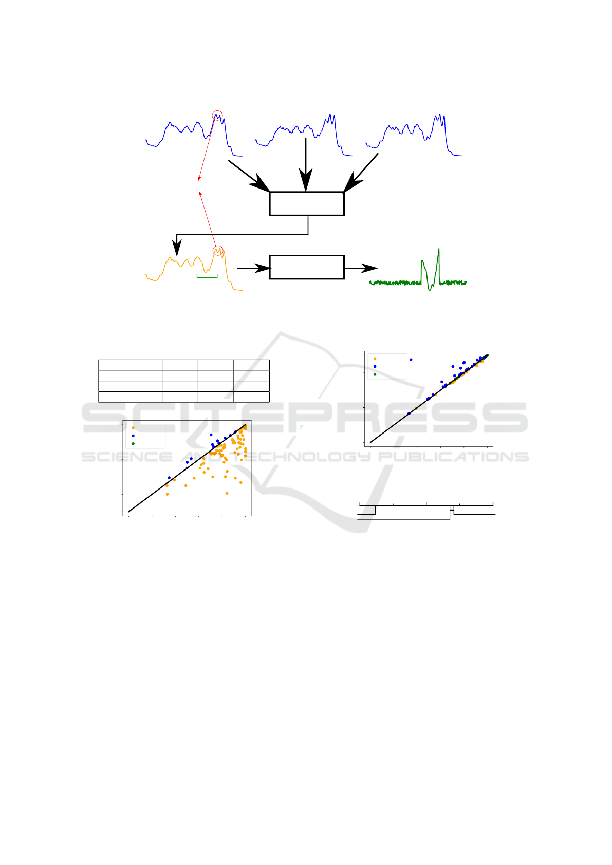
of the pos sample generation can be seen in Figure 3.

We note that during training, the triplet generation

is done in an online way at each epoch in order to

make the model generalize better.

Enhancing Time Series Classiﬁcation with Self-Supervised Learning

Algorithm 1: Triplet Generation.

1: Input: data

2: shufﬂe(data)

3: N ← data.shape[0] ▷ Number of samples in data

4: l ← data.shape[1] ▷ Length of input samples

5: w ← random(0.6,1) ▷ The amount of mixing up

contribution

6: for i : 0 → N do

7: re f [i] ← data[i]

8: ts

← random sample(data)

9: ts

← random sample(data)

10: pos[i] ← w.re f [i] + (

1−w

).(ts

+ts

)

11:

12: ts

← random sample(data)

13: ts

← random sample(data)

14: ts

← random sample(data)

15: neg[i] = w.ts

+ (

1−w

).(ts

+ts

)

16:

17: pos[i], neg[i] ← Mask(pos[i], neg[i])

18: end for

19: pos ← Znormalize(pos)

20: neg ← Znormalize(neg)

21: return re f , pos, neg

Algorithm 2: Mask.

1: Input: x, y

2: Output: x, y

3: l ← len(x)

4: start ← random randint(0, l − 1)

5: stop ← random randint(start +

l−1−start

, start +

l−1−start

2.5

)

6: x[0 : start] ← noise

7: x[stop + 1 :] ← noise

8: y[0 : start ← noise

9: y[stop + 1 :] ← noise

10: return x,y

4 EXPERIMENTAL

EVALUATIONS

In this section we evaluate the proposed model con-

sidering the two use cases identiﬁed in Section 1.

4.1 Datasets and Implementation

Details

We based all of our experiments on the UCR

archive (Dau et al., 2019) which is the largest open

source archive for TSC. We used the 2015 version

of the UCR archive made of 85 univariate time se-

ries. We z-normalized the datasets before applying

our TRILITE model. All of the results are averaged

on ﬁve runs. We used the Adam optimizer with an

initial learning rate of 10

−3

. For the choice of the

hyperparameter α, we tried to tune it on the set of

values {10

−6

, 10

−5

, 10

−4

, 10

−3

, 10

−2

, 10

−1

}. We ob-

served, by visualizing the latent representations, that

when we change the value of α the model changes

the scale of the representations. By this change of

scale, the type of the triplet (as explained in Sec-

tion 2) would not change. After this observations

we ﬁxed the value of α to 10

−2

tuned on a sub-

set of the UCR archive. We trained the model for

1000 epochs with a batch size of 32. For the evalu-

ation on the test set, we used the last model. We did

the experiments on a NVIDIA GeForce GTX 1080

with 8GB of memory. The code is publicly available

https://github.com/MSD-IRIMAS/TRILITE.

4.2 Use Case 1: Small Annotated Time

Series Datasets

To address this ﬁrst case where a small annotated time

series dataset is available, we compared the TRILITE

model, followed by a fully connected layer with soft-

max activation (denoted as TRILITE 1-LP), with the

single FCN. The Win-Tie-Loss visualization is re-

ported in Figure 4. We can observe that not sur-

prisingly, the supervised model outperforms the self-

supervised one. However, for some datasets we can

see that self-supervised features allow to improve the

classiﬁcation accuracy (blue points). This motivated

us to evaluate the contribution of self-supervised fea-

tures in a supervised problem. In order to do that we

simply concatenate the latent representations of the

self-supervised TRILITE model (of size 128) and the

latent representations of the supervised FCN model

(of size 128) for the train and test sets. Then, these

concatenated features are fed to a classiﬁer, a one

fully connected layer with a softmax activation. We

compare this approach, denoted as TRILITE+FCN,

with the single FCN and the single TRILITE mod-

els. For each model we compute the classiﬁcation

accuracy and rank them accordingly on each dataset.

Ranking results are reported in Table 1 and visual-

ized in the Critical Difference Diagram in Figure 6.

These results show that the TRILITE+FCN approach

occurs at the ﬁrst rank position more often than the

single FCN model. This is emphasized in the Win-

Tie-Loss comparison in Figure 5. We can see that the

TRILITE+FCN approach is never worse than the sin-

gle FCN in a signiﬁcant manner. This is due to the

fact that supervised features can not get perturbed by

the SSL features. In the worst case scenario, the linear

classiﬁer can learn to reject the SSL features in case

ICAART 2023 - 15th International Conference on Agents and Artiﬁcial Intelligence

MixUp

Mask

mixed information

Masking

interval

ref

TS1

TS2

pos

pos masked

Figure 3: A pos (in orange) is built from three time series including the re f (in blue). The resulting time series is close to

the re f except some areas as highlighted in the red circle. A mask is then applied on the mixed up pos to generate the ﬁnal

sample (in green), where the unmasked parts are replaced by a Gaussian noise.

Table 1: Ranking each method on the 85 UCR archive

datasets.

Method Rank 1 Rank 2 Rank 3

TRILITE 1-LP 8 4 73

FCN 37 37 11

TRILITE+FCN 40 44 1

0 20 40 60 80 100

FCN

100

TRILITE 1-LP

TRILITE 1-LP VS FCN

Loss 73

Win 12

Tie 0

FCN is

better here

TRILITE 1-LP

is better here

Figure 4: TRILITE with 1-LP VS supervised FCN.

they were perturbing the classiﬁcation. In addition, on

average, the difference in accuracy is 3.73 + −9.94

when TRILITE+FCN wins. Conversely, the differ-

ence in accuracy is only 0.64 + −0.7 when the single

FCN wins. This shows that SSL produces features

different than the ones produced by supervised learn-

ing. As a result, the concatenation of both features

allows to improve the classiﬁcation performance.

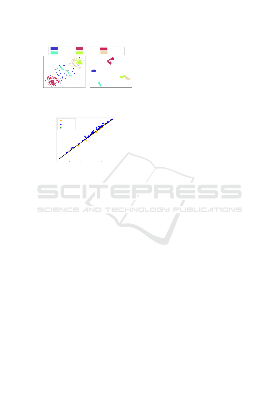
This suggests that the self-supervised model is

able to discriminate between classes even if it was not

it’s main objective during training. To emphasize this,

we employed T-distributed Stochastic Neighbor Em-

bedding (TSNE) (Van der Maaten and Hinton, 2008)

to visualize a two-dimensional space representing the

raw data and the self-supervised features (Figure 7)

for the SyntheticControl dataset of the UCR archive.

0 20 40 60 80 100

FCN

100

TRILITE+FCN

TRILITE+FCN VS FCN

Loss 38

Win 39

Tie 8

TRILITE+FCN

is better here

FCN is

better here

Figure 5: Concatenation with 1-LP VS supervised FCN.

123

2.7647

1.6471

FCN

1.5882

TRILITE+FCN

TRILITE 1-LP

Accuracy

Figure 6: Average rank mean of the three methods on 84

datasets of the UCR archive.

In the later ﬁgure, we can clearly identify distinct and

compact clusters representing the classes.

4.3 Use Case 2: Partially Annotated

Time Series Datasets

In this second case where, we consider a semi-

supervised scenario where only a part of the data is

labeled. We aim to evaluate how SSL can overcome

this lack of labels. To do that we follow these differ-

ent steps supposing that only 30% of the training set

is labeled:

1. Self-supervised training. We obtain self-

supervised latent representations by training our

Enhancing Time Series Classiﬁcation with Self-Supervised Learning

-10

-20

-5-10

-15

-5

TSNE on raw samples

TSNE on latent representation

Class -1.0-

Class -2.0-

Class -3.0-

Class -4.0-

Class -5.0-

Class -6.0-

-10

-20

-10

Figure 7: TSNE representation on the SyntheticControl

dataset on raw samples and TRILITE latent representation.

0 20 40 60 80 100

Experiment 1

100

Experiment 2

Experiment 1 VS Experiment 2

Loss 29

Win 56

Tie 0

Experiment 1

is better here

Experiment 2

is better here

Figure 8: Comparison of experiment 1 (1a) and experiment

2 (1b). In experiment 1, the TRILITE model is trained only

on the labeled subset (30% of the data). On the contrary, in

experiment 2, the TRILITE model is trained on the whole

train set. The evaluation is done on the whole test set.

TRILITR model:

(a) experiment 1: only on the labeled subset.

(b) experiment 2: on the whole training set.

2. Supervised learning. We feed the latent represen-

tations of the labeled set (either 1a or 1b) to a

Ridge classiﬁer (Peng and Cheng, 2020).

3. Evaluation. The trained classiﬁer is evaluated on

the test set.

To not be dependent on a single labeled subset, these

steps are repeated over 25 runs and the average ac-

curacy is computed. For each run, the same labeled

subset is used for both experiments The Win-Tie-Loss

comparison between experiments 1 and 2 is shown in

Figure 8.

We can see that experiment 2 obtains more wins

than experiment 1. In addition, on average, the differ-

ence in accuracy when experiment 2 wins is 2.12 +

−2.13. On the contrary when experiment 1 wins, the

difference in accuracy is on average of 1.17 + −1.21.

This shows that SSL can learn a more meaningful la-

tent representation when taking into consideration the

labeled and unlabeled subsets.

5 CONCLUSION

The difﬁculty to annotate time series data often results

in a lack of labeled data, and thus complicates the

training of supervised TSC models. In this paper, we

proposed a Self-Supervised approach for TSC in or-

der to address this problem. In particular, trough two

use cases, we evaluated how Self-Supervised Learn-

ing can be employed in combination with supervised

learning to enhance TSC performances. First, we

consider the case of small annotated datasets. We

showed that with the help of self-supervision, the per-

formance of supervised learning can be improved in

some cases. Second, in a case partially annotated

datasets, we showed that Self-Supervised Learning

can also be a complement to learning supervised mod-

els only on labeled data. Hence, these experimental

results demonstrated that our SSL approach allows

to capture meaningful features that are complemen-

tary to features captured in supervised models. The

main problem we faced is how to evaluate the self-

supervised models, which architecture to use, which

data augmentation to apply and which loss to mini-

mize. Furthermore, we aim to study the impact of

each hyperparameter on the problem at hand when us-

ing Self-Supervised Learning.

ACKNOWLEDGEMENTS

This work was supported by the ANR DELEGATION

project (grant ANR-21-CE23-0014) of the French

Agence Nationale de la Recherche. The authors

would like to acknowledge the High Performance

Computing Center of the University of Strasbourg

for supporting this work by providing scientiﬁc sup-

port and access to computing resources. Part of the

computing resources were funded by the Equipex

Equip@Meso project (Programme Investissements

d’Avenir) and the CPER Alsacalcul/Big Data. The

authors would also like to thank the creators and

providers of the UCR Archive.

REFERENCES

Anowar, F., Sadaoui, S., and Dalal, H. (2022). Cluster-

ing quality of a high-dimensional service monitoring

time-series dataset. In ICAART (2), pages 183–192.

Ay, E., Devanne, M., Weber, J., and Forestier, G. (2022).

A study of knowledge distillation in fully convolu-

tional network for time series classiﬁcation. In Int.

Joint Conference on Neural Networks (IJCNN).

Chen, T., Kornblith, S., Norouzi, M., and Hinton, G. (2020).

A simple framework for contrastive learning of visual

ICAART 2023 - 15th International Conference on Agents and Artiﬁcial Intelligence

representations. In Int. conference on machine learn-

ing, pages 1597–1607. PMLR.

Chen, Y., Zhou, X., Xing, Z., Liu, Z., and Xu, M. (2022).

Cass: A channel-aware self-supervised representation

learning framework for multivariate time series classi-

ﬁcation. In Int. Conference on Database Systems for

Advanced Applications, pages 375–390. Springer.

Dau, H. A., Bagnall, A., Kamgar, K., Yeh, C.-C. M., Zhu,

Y., Gharghabi, S., Ratanamahatana, C. A., and Keogh,

E. (2019). The ucr time series archive. IEEE/CAA

Journal of Automatica Sinica, 6(6):1293–1305.

Deng, J., Dong, W., Socher, R., Li, L.-J., Li, K., and Fei-

Fei, L. (2009). Imagenet: A large-scale hierarchical

image database. In 2009 IEEE conference on com-

puter vision and pattern recognition, pages 248–255.

Ieee.

Eldele, E., Ragab, M., Chen, Z., Wu, M., Kwoh, C. K.,

Li, X., and Guan, C. (2021). Time-series representa-

tion learning via temporal and contextual contrasting.

arXiv preprint arXiv:2106.14112.

Fawaz, H. I., Forestier, G., Weber, J., Idoumghar, L., and

Muller, P.-A. (2018). Data augmentation using syn-

thetic data for time series classiﬁcation with deep

residual networks. arXiv preprint arXiv:1808.02455.

Franceschi, J.-Y., Dieuleveut, A., and Jaggi, M. (2019). Un-

supervised scalable representation learning for multi-

variate time series. Advances in neural information

processing systems, 32.

Garg, Y. (2021). Retrim: Reconstructive triplet loss for

learning reduced embeddings for multi-variate time

series. In 2021 Int. Conference on Data Mining Work-

shops (ICDMW), pages 460–465. IEEE.

Grill, J.-B., Strub, F., Altch

e, F., Tallec, C., Richemond, P.,

Buchatskaya, E., Doersch, C., Avila Pires, B., Guo,

Z., Gheshlaghi Azar, M., et al. (2020). Bootstrap your

own latent-a new approach to self-supervised learn-

ing. Advances in Neural Information Processing Sys-

tems, 33:21271–21284.

He, K., Zhang, X., Ren, S., and Sun, J. (2016). Deep resid-

ual learning for image recognition. In Proceedings of

the IEEE conference on computer vision and pattern

recognition, pages 770–778.

Hinton, G., Vinyals, O., Dean, J., et al. (2015). Distilling

the knowledge in a neural network.

Ismail Fawaz, H., Forestier, G., Weber, J., Idoumghar, L.,

and Muller, P.-A. (2019). Deep learning for time series

classiﬁcation: a review. Data mining and knowledge

discovery, 33(4):917–963.

Ismail Fawaz, H., Lucas, B., Forestier, G., Pelletier, C.,

Schmidt, D. F., Weber, J., Webb, G. I., Idoumghar, L.,

Muller, P.-A., and Petitjean, F. (2020). Inceptiontime:

Finding alexnet for time series classiﬁcation. Data

Mining and Knowledge Discovery, 34(6):1936–1962.

Kavran, D., Zalik, B., and Lukac, N. (2022). Time series

augmentation based on beta-vae to improve classiﬁca-

tion performance. In ICAART (2), pages 15–23.

Lafabregue, B., Weber, J., Ganc¸arski, P., and Forestier, G.

(2022). End-to-end deep representation learning for

time series clustering: a comparative study. Data Min-

ing and Knowledge Discovery, 36(1):29–81.

LeCun, Y., Bottou, L., Bengio, Y., and Haffner, P. (1998).

Gradient-based learning applied to document recogni-

tion. Proceedings of the IEEE, 86(11):2278–2324.

Liang, Y., Pan, Y., Lai, H., Liu, W., and Yin, J. (2021).

Deep listwise triplet hashing for ﬁne-grained image

retrieval. IEEE Transactions on Image Processing.

Lin, L., Song, S., Yang, W., and Liu, J. (2020). Ms2l: Multi-

task self-supervised learning for skeleton based action

recognition. In Proceedings of the 28th ACM Int. Con-

ference on Multimedia, pages 2490–2498.

Mercier, D., Bhatt, J., Dengel, A., and Ahmed, S. (2022).

Time to focus: A comprehensive benchmark us-

ing time series attribution methods. arXiv preprint

arXiv:2202.03759.

Mohsenvand, M. N., Izadi, M. R., and Maes, P. (2020).

Contrastive representation learning for electroen-

cephalogram classiﬁcation. In Machine Learning for

Health, pages 238–253. PMLR.

Oki, H., Abe, M., Miyao, J., and Kurita, T. (2020). Triplet

loss for knowledge distillation. In 2020 Int. Joint

Conference on Neural Networks (IJCNN), pages 1–7.

IEEE.

Peng, C. and Cheng, Q. (2020). Discriminative ridge ma-

chine: A classiﬁer for high-dimensional data or imbal-

anced data. IEEE Transactions on Neural Networks

and Learning Systems, 32(6):2595–2609.

Pialla, G., Devanne, M., Weber, J., Idoumghar, L., and

Forestier, G. (2022a). Data augmentation for time

series classiﬁcation with deep learning models. In

Advanced Analytics and Learning on Temporal Data

(AALTD), page undeﬁned. undeﬁned.

Pialla, G., Fawaz, H. I., Devanne, M., Weber, J., Idoumghar,

L., Muller, P.-A., Bergmeir, C., Schmidt, D., Webb,

G., and Forestier, G. (2022b). Smooth perturbations

for time series adversarial attacks. In Paciﬁc-Asia

Conference on Knowledge Discovery and Data Min-

ing, pages 485–496. Springer.

Schroff, F., Kalenichenko, D., and Philbin, J. (2015).

Facenet: A uniﬁed embedding for face recognition

and clustering. In Proceedings of the IEEE conference

on computer vision and pattern recognition, pages

815–823.

Terefe, T., Devanne, M., Weber, J., Hailemariam, D., and

Forestier, G. (2020). Time series averaging using

multi-tasking autoencoder. In 2020 IEEE 32nd Int.

Conference on Tools with Artiﬁcial Intelligence (IC-

TAI), pages 1065–1072. IEEE.

Van der Maaten, L. and Hinton, G. (2008). Visualizing data

using t-sne. Journal of machine learning research,

9(11).

Wang, Z., Yan, W., and Oates, T. (2017). Time series clas-

siﬁcation from scratch with deep neural networks: A

strong baseline. In 2017 Int. joint conference on neu-

ral networks (IJCNN), pages 1578–1585. IEEE.

Wickstrøm, K., Kampffmeyer, M., Mikalsen, K. Ø., and

Jenssen, R. (2022). Mixing up contrastive learning:

Self-supervised representation learning for time se-

ries. Pattern Recognition Letters, 155:54–61.

Yang, X., Zhang, Z., and Cui, R. (2022). Timeclr: A self-

supervised contrastive learning framework for univari-

ate time series representation. Knowledge-Based Sys-

tems, page 108606.

Enhancing Time Series Classiﬁcation with Self-Supervised Learning