A Patch-Based Architecture for Multi-Label Classiﬁcation from Single

Positive Annotations

Warren Jouanneau

1,2

, Aur

elie Bugeau

2,3

, Marc Palyart

, Nicolas Papadakis

and Laurent V

ezard

Lectra, F-33610 Cestas, France

Univ. Bordeaux, Bordeaux INP, CNRS, LaBRI, UMR 5800, F-33400 Talence, France

Institut Universitaire de France (IUF), France

Univ. Bordeaux, Bordeaux INP, CNRS, IMB, UMR 5251, F-33400 Talence, France

Keywords:

Partial and Unlabeled Learning, Patch-Based Method, Classiﬁcation.

Abstract:

Supervised methods rely on correctly curated and annotated datasets. However, data annotation can be a cum-

bersome step needing costly hand labeling. In this paper, we tackle multi-label classiﬁcation problems where

only a single positive label is available in images of the dataset. This weakly supervised setting aims at simpli-

fying datasets assembly by collecting only positive image exemples for each label without further annotation

reﬁnement. Our contributions are twofold. First, we introduce a light patch architecture based on the attention

mechanism. Next, leveraging on patch embedding self-similarities, we provide a novel strategy for estimat-

ing negative examples and deal with positive and unlabeled learning problems. Experiments demonstrate that

our architecture can be trained from scratch, whereas pre-training on similar databases is required for related

methods from the literature.

1 INTRODUCTION

Data annotation, or labelling, is at the core of super-

vised learning approaches. In image classiﬁcation,

state-of-the-art methods rely on an ever-increasing

amount of data, which makes the annotation collec-

tion a major issue. Training datasets are made of

image-label associations obtained from an expensive

manual annotation, an automatic collection, or ﬁlter-

ing and mapping of existing image descriptions. As-

sembling a dataset is difﬁcult, especially when: ex-

perts must annotate unlabelled data; rare events have

to be recognized; or a dataset is created from different

sources with inconsistent label taxonomies.

The accurate characterization of most images re-

quires multi-label classiﬁcation. Image content is in-

deed rich in information, as it includes multiple struc-

tured components. Associating a single label to an

image is a too restricted setting. It is preferable to an-

notate an image with several and non-exclusive labels

(e.g. presence/absence of wood, metal, fabric, etc.).

For supervised learning purpose, positive and neg-

ative examples for each label are needed in the train-

ing dataset. The image-labels associations need to be

exhaustive. Any missing or incorrect annotation for

the label l on a given image X leads to a wrong ex-

ample for this label. Such errors may have an im-

pact on the complete labelling of the image X, and

on the characterization of the label l on the remain-

ing images of the dataset. Naturally, obtaining er-

ror free multi-label annotations makes the dataset cre-

ation more complex. To alleviate the task of dataset

creation, weakly supervised learning methods only

rely on partial data annotations. Such methods com-

bine approaches ranging from fully supervised to un-

supervised learning, e.g. few shot learning where only

a small set of examples is available for each label.

A special case of weak supervision for classiﬁca-

tion is positive and unlabeled (PU) learning (Bekker

and Davis, 2020). In PU learning, only partial positive

labeling is available. In the multi-label PU setting, the

training data contain only a single label for each im-

age, whereas several labels can be present in each im-

age Hence, only a subset of images of the training data

set are annotated for each label. For the remaining im-

ages, we have no information, which means that we

do not know if a label is present or not in the image.

In the multi-label positive and unlabeled learning con-

text, obtaining annotations is greatly simpliﬁed. PU

learning is indeed adapted to automatic data collec-

tion and dataset merging. Positive examples for each

label can be collected independently of what they rep-

resent for other labels. More generally, as it does not

require negative examples and annotation complete-

ness, PU is well suited to handle heterogeneous label-

ings coming from different datasets.

Jouanneau, W., Bugeau, A., Palyart, M., Papadakis, N. and Vézard, L.

A Patch-Based Architecture for Multi-Label Classiﬁcation from Single Positive Annotations.

DOI: 10.5220/0011610800003417

In Proceedings of the 18th International Joint Conference on Computer Vision, Imaging and Computer Graphics Theor y and Applications (VISIGRAPP 2023) - Volume 5: VISAPP, pages

47-58

ISBN: 978-989-758-634-7; ISSN: 2184-4321

 2023 by SCITEPRESS – Science and Technology Publications, Lda. Under CC license (CC BY-NC-ND 4.0)

In PU learning, one difﬁculty is to deal with the

absence of negative examples. The situation is even

worse in the multi-label context, where each image is

actually both positive for certain labels and negative

for other ones.

1.1 Problem Setting and Methodology

We face the multi-label PU learning which is a multi-

label classiﬁcation problem where each image may

contain zero, one or several objects from one or sev-

eral different categories. Moreover, in our use cases,

only one positive label per image is used during train-

ing, and no negative labels are available.

In this work, we propose to address the absence of

negative examples in training datasets with a patch-

based approach. Following (Trockman and Kolter,

2022), we argue that the patch level can be better

suited than the image level to achieve multi-label

characterization in the case of PU learning. More pre-

cisely, we use the fact that when an image is a posi-

tive example regarding a given label, then some of its

patches can be considered positives for this label, and

other ones negatives. When training examples only

contain positive labeling at the image level, the patch-

label association is nevertheless unknown.

1.2 Contributions and Outline

Our main contribution, presented in section 3 is a

light patch-based architecture adapted to multi-label

PU learning. By considering an image as a set of

patches, we build multi-label image representations

with a patch attention mechanism. Assuming that a

small image patch mostly contains a single class label,

our architecture allows the estimation of negative ex-

amples by leveraging on patch-based image represen-

tation self-similarities. This is a main novelty, as the

negative examples estimated by existing approaches

for PU learning (Cole et al., 2021; Verelst et al., 2022)

are based on the prediction score at the image level

without relying on the local data content.

In section 4, experiments demonstrate that our

patch-based framework is adapted to multi-label clas-

siﬁcation problems with single positive annotations,

while providing an explicit spatial localization of la-

bels. When training models from scratch, our archi-

tecture generalizes faster and better than Resnet-5,

while being signiﬁcantly lighter (reduction ×100 of

the number of parameters).

2 RELATED WORKS

In this section, we ﬁrst review multi-label classiﬁca-

tion models using set of patches. Next, we discuss ex-

isting strategies to obtain a global image representa-

tion from the information contained in a set of patches

and their embeddings. Finally, we present state-of-

the-art methods for positive and unlabeled learning.

2.1 Patch Embeddings for Multi-Label

Image Classiﬁcation

Multi-label classiﬁcation of images can be split into

multiple single label classiﬁcation tasks (Read et al.,

2009), where each classiﬁer is in charge of predict-

ing a speciﬁc label. Recent works demonstrate the

interest of tackling the joint multi-label problem (Wei

et al., 2014). In image data, there is indeed a cor-

relation between localization and labels. As a con-

sequence, detection methods not only intend to in-

fer the image labels, but they also aim at estimat-

ing their localization through bounding boxes (Ren

et al., 2015; Redmon et al., 2016) or segmentation

masks (He et al., 2017).

Considering an image as a set of patches is an

appropriate model for multi-label classiﬁcation. In

practical applications, unless a hierarchical label tax-

onomy is considered (hairs, head, body), labels are

indeed related to a subpart of the image only (e.g.

wood, brick, metal...). With a patch-based approach,

each patch specializes and contributes to the classiﬁ-

cation with respect to a single label. Patch-based ap-

proaches have been introduced for texture synthesis

problems (Efros and Leung, 1999). Their interest has

been demonstrated for image level tasks such as de-

noising (Buades et al., 2005), super-resolution (Free-

man et al., 2002), segmentation, labeling (Coup

et al., 2011), classiﬁcation (Varma and Zisserman,

2008), etc. In particular, the representation of an im-

age from its extracted patches has been thoroughly

studied, and we refer the reader to (Liu et al., 2019)

for a review of methods from the bag-of-word frame-

work to recent deep models.

The Transformer architecture (Vaswani et al.,

2017), originally proposed for natural language pro-

cessing, has soon been transposed to image tasks. In

order to adapt Transformer architecture to images, the

ViT method (Dosovitskiy et al., 2020) considers an

image as a set of patches or as a sequence (if patch

position is encoded) of patches. The ViT achieves

impressive results without convolution layers. Many

extensions of the image Transformer focus on the

construction of a relevant set of elements to feed to

the network. As an example, CrossViT (Chen et al.,

VISAPP 2023 - 18th International Conference on Computer Vision Theory and Applications

2021) relies on patches of different size, which brings

multi-scale information. In other works, a convolu-

tion neural network (CNN) can be used as a stem

(Xiao et al., 2021) or as a feature pyramid (Zhang

et al., 2020) to feed a Transformer network.

Relying on sets of patch embeddings proved to

be a powerful methodology for image classiﬁcation

with modern learning methods. The ConvMixer

model (Trockman and Kolter, 2022) shows for in-

stance that Transformers’ performances are mostly

due to the representation of images as a set of patches,

rather than to the architecture itself. When facing

image classiﬁcation problems, one has to come back

from patch level to image level at some point.

2.2 From Set of Patch Embeddings to

Image Representation

We now present methods providing a relevant image

representation from the embeddings of image patches.

Image representation must handle multi-label classi-

ﬁcation and deal with the presence of multiple in-

stances of these labels in the images. To that end, the

information contained in the set of embedded patches

has to be aggregated. In the literature, the aggrega-

tion of elements in a set is mainly done using pooling

operator such as average, max, min or sum of the ele-

ment representations (Zaheer et al., 2017). The pool-

ing of feature maps related to receptive ﬁelds of dif-

ferent sizes is for instance usually done with global

average (Lin et al., 2013).

The raise in popularity of the attention mechanism

has led to new pooling methods (Ilse et al., 2018)

realizing weighted sums of element representations.

Transformers (Vaswani et al., 2017), relying on multi-

head attention, can also operate as element pooling.

The transformer uses cross-attention with weights

given by a similarity score between the element rep-

resentations and ”queries”. In the case of patches,

these ”queries” can be seen as codebooks (Zhao et al.,

2022). Queries can be designed beforehand, or they

can be parameters learned by the model. A main lim-

itation of the transformer is its quadratic complexity

with respect to the dimension of input data. In order to

reduce the computational burden of transformers, the

perceiver (Jaegle et al., 2021) architecture computes

intermediate latent representations of reduced dimen-

sion before realizing cross-attentions with the queries.

Hence, a task dependent element pooling can be con-

sidered for each query. The queries can therefore be

deﬁned as label embeddings (Lanchantin et al., 2021),

with an independent pooling for each label.

In computer vision, multiple instance learning

consists in both detecting the presence of a label at

the image level and localizing accurately the corre-

sponding instances (Carbonneau et al., 2018). The at-

tention mechanism provides a joint solution to these

problems (Ilse et al., 2018), as element pooling nat-

urally deals with multiple instances of a label in an

image. The detection of a label is indeed given by

the pooling of the patch embeddings with the cor-

responding query. The similarity weight between a

patch and a query indicates the degree of participa-

tion of the patch in the label decision. If a patch has

an important weight in the pooling of a label predicted

as positive, then this patch should contain relevant in-

formation relative to this label. As a consequence, the

similarity weights can help to localize distinct subar-

eas of the image corresponding to a single label.

In a supervised setting, patch attention mechanism

is adapted to both multi-label and multiple instance

cases. However, its application to weakly supervised

problems with positive only annotations at the image

level requires the development of new methods.

2.3 Positive and Unlabeled Learning for

Multi-Label Classiﬁcation

Positive and unlabeled (PU) classiﬁcation is a weakly

supervised classiﬁcation problem where only posi-

tive examples are available. As studied in the re-

view (Bekker and Davis, 2020), many methods have

addressed this problem in the single-label setting.

However, only few methods dedicated to PU

learning for multi-label classiﬁcation problems exist.

As detailed in (Cole et al., 2021), most works con-

sider the many (and not single) positive (Kanehira

and Harada, 2016) case, the single positive or nega-

tive one (Huang and Yan, 2018) or the existence of

negatives for each label (Ishida et al., 2017).

In this paper, we focus on the complex multi-

label application case where only a single positive

label is known for each element of the training set.

In (Mac Aodha et al., 2019), all but the known pos-

itive examples are considered as negatives and in-

cluded as groundtruth negative examples in the loss

function optimized during training. This corresponds

to a uniform penalization of the positive predictions,

that can be enhanced with a dedicated spatial consis-

tency loss (Verelst et al., 2022). Cole et al. (Cole

et al., 2021) propose to enhance this kind of meth-

ods with the Regularized Online Label Estimation

(ROLE) strategy. The ROLE model ﬁrst improves

the loss function with a term penalizing the distance

between the number of positive label predictions for

an image and a hyperparameter. This hyperparame-

ter corresponds to the mean number of positive labels

per image that is nevertheless unknown in general.

A Patch-Based Architecture for Multi-Label Classiﬁcation from Single Positive Annotations

Then, an online label estimation strategy is consid-

ered for unobserved labels. It consists in learning new

parameters that should correspond to the groundtruth

value of unknown labels, that can be either positive or

negative. These estimations are realized in a separate

branch of the model and are compared with the actual

predictions of the model in a dedicated loss.

The ROLE model (Cole et al., 2021) makes an

interesting proposition with the online estimation of

negative examples. Nevertheless, it does not lever-

age on data content to provide negative examples and

tackle the multi-label aspect of the problem. The on-

line strategy mainly stabilizes the learning through

memorization of former label predictions. In prac-

tice, it reinforces the tendencies (positive or negative

predictions) provided by the current model, by mak-

ing the predicted weight values closer and closer to

0 or 1. We argue that the patch-based approach is a

suitable strategy to estimate negative examples in the

context of multi-label PU learning.

3 METHODOLOGY

We start this section with a formal statement of the

multi-label classiﬁcation problem addressed in this

paper. Given a set of labels l ∈ L, the objective is to

determine P(x

|l), the probability of presence of the

label l in an image x

. We denote as y

= {y

n,l

}

l∈L

the ground truth labels that indicate if a class l ∈ L

is present (y

n,l

= 1) or not (y

n,l

= 0) in an image

. Hence, the multi-label problem can be formulated

as the estimation of a labeling score

= { ˆy

n,l

}

l∈L

where ˆy

n,l

∈ [0, 1] indicates the presence ( ˆy

n,l

→ 1) or

absence ( ˆy

n,l

→ 0) of the label l in the image x

Training multi-label classiﬁcation in a fully-

supervised manner requires entirely annotated data,

for which the collection and annotation are costly. In

our case, this complete annotation is not available.

We have partial ground truth annotations on an image

dataset containing partial positive z

and negative z

−

examples for the image x

. We consider that z

n,l

= 1

(resp. z

n,l

= 1) means that the label l is present (resp.

absent) in the annotated image x

. If z

n,l

= z

n,l

= 0

then we have no information on the label l. Finally,

the two annotated sets are assumed compatible, so

that the case z

n,l

= z

n,l

= 1 is impossible.

In the Positive and Unlabeled (PU) context con-

sidered in this paper, nothing is known about the neg-

atives (z

n,l

= 0 for all n and l) and the positive la-

bels are only partially observed. In our applications,

we nevertheless consider that one single positive label

n,l

= 1 is available per image x

To solve the multi-label PU problem, we propose

a weakly supervised method that relies on the use of

image patches. It is built on top of a key hypothesis: a

small enough image patch is mostly characteristic of

only one single label.

In section 3.1, we describe our patch-based ar-

chitecture for multi-label classiﬁcation. Section 3.2

presents the loss proposed to train the model. In sec-

tion 3.3, we build on our patch-based architecture to

provide negative examples and deal with PU learning.

Why a New Patch Architecture for PU Learning?.

In section 3.1, we propose a new patch architecture

adapted to multi-label learning problems, where only

(partial) positive labels are available in the training

set. Classical models such as ViT (Dosovitskiy et al.,

2020) rely on one global image representation for

the classiﬁcation task. The embedding obtained for

a given image and a given label thus contains infor-

mation coming from all areas of the image, including

areas that are relevant for other labels. Hence it is dif-

ﬁcult to characterize negative examples for a single

label (i.e. images that are negative detections for one

label) using these global image embeddings.

In this work, as in ConvMixer (Trockman and

Kolter, 2022), we rather represent an image with a

subset of its patches. Contrary to ConvMixer that con-

siders a global image representation, we build differ-

ent image representations, one per class label. More-

over, all embeddings lives in the same latent space,

that are composed of embedded features extracted

from different subsets of patches. Thanks to this com-

mon latent space, subsets of patches can be easily ob-

tained by only selecting image patches that are rele-

vant for each label. As we later demonstrate in sec-

tion 3.2, such a model leads to a new and simple

scheme for estimating negative examples at the patch

level. As a by-product, it also allows for the localiza-

tion of detected labels within images

3.1 Patch-Based Architecture

We now provide a detailed description of our patch-

based architecture. As illustrated in Figure 1, the ar-

chitecture is composed of ﬁve blocks based on the

bag-of-word framework. A subset of patch is ﬁrst se-

lected. The patches are then embedded in a general

representation space, in which also live label code-

books. A pooling of the patch embedding for each la-

bel is then performed using an attention mechanism.

It is followed by the ﬁnal multi-label classiﬁcation.

3.1.1 Patch Extraction

(Block 1 of ﬁgure 1): An image is ﬁrst converted

into a set of patches extracted at different resolutions.

VISAPP 2023 - 18th International Conference on Computer Vision Theory and Applications

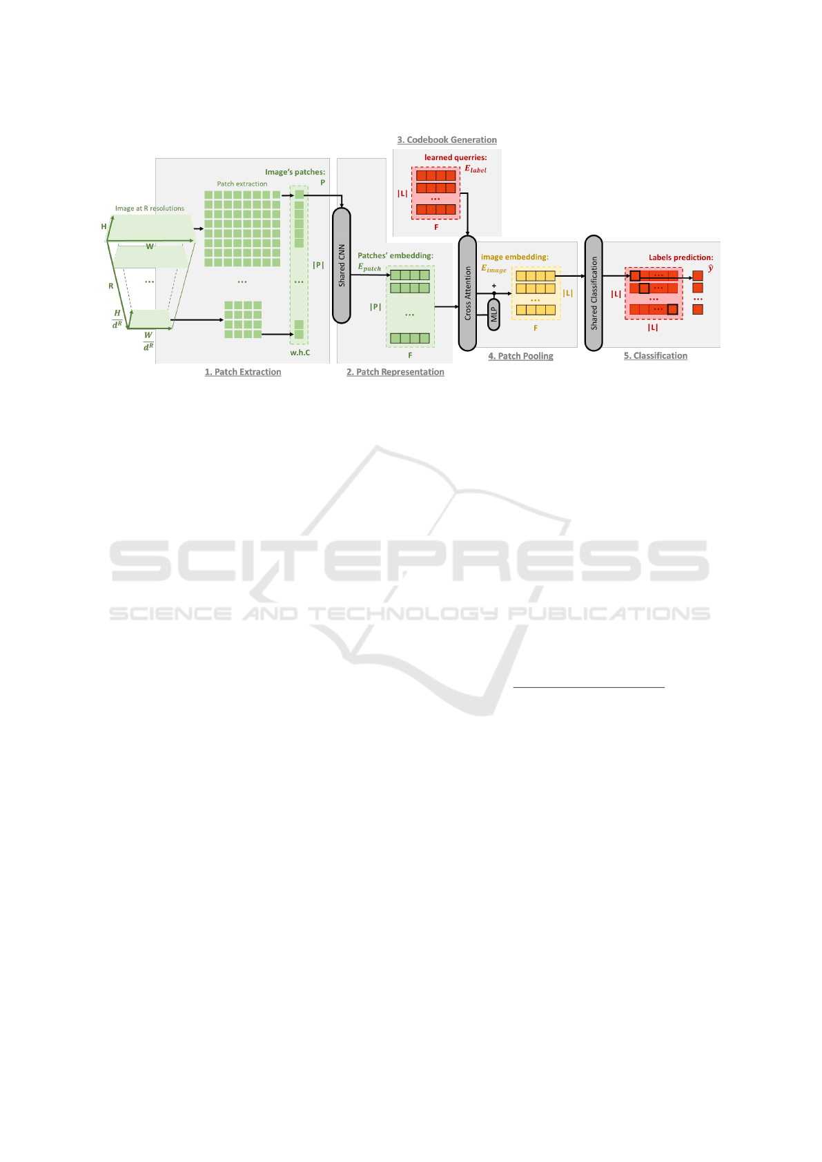
Figure 1: Proposed multi-resolution patch deep neural network architecture.

Each image I ∈ R

H×W×C

of height H, width W and

with C channels is downsampled spatially R times

with a constant uniform ratio d, using bilinear inter-

polation. For each resulting image, patches P are ex-

tracted using a sliding window looping through the

image both horizontally (W) and vertically (H) with

a uniform window size h × w and stride. At each res-

olution, we denote a patch p ∈ R

h×w×C

. The patch

size being the same across all resolutions, the set of

patches contain ﬁne to coarse information with de-

creasing resolution. In this work, we consider the

same size for the stride and the sliding windows, so

that patches form a perfect grid of the image. When

the image size is too large, patches can be randomly

subsampled at each resolution level to limit the com-

putational burden.

3.1.2 Patch Representation

(Block 2 of ﬁgure 1): Each patch is fed into a CNN

architecture. The weights of this model are shared

across all patches. With this backbone model, all

m patches are projected into the same latent space

of dimension F, E

patch

= {e

patch

| e

patch

∈ R

, i =

1·· · m}, resulting in a vector of embedded features

patch

∈ E

patch

that play the role of patch descriptors.

The CNN architecture consists of multiple efﬁcient-

Net blocks (Tan and Le, 2019).

3.1.3 Codebook Embedding

(Block 3 of ﬁgure 1): Each label is associated with

its own representative patch, e

label

, that we call code-

book. We assume that each representation e

label

con-

tains the embedded feature that a patch should con-

tain to be discriminated as positive in regard to the

corresponding label l. The set of all codebooks, de-

noted, E

label

= {e

label

| e

label

∈ R

, l ∈ L}, is obtained

through back-propagation.

3.1.4 Image Representations with Patch Pooling

(Block 4 of ﬁgure 1): An image representation is cre-

ated from the embedded patches. To that end, we

propose to consider attention pooling. The pooling

is done using cross-attention between the set E

patch

of embedded patches and the learned label codebooks

label

. This attention mechanism can be seen as a two

steps approach. The ﬁrst step consists in evaluating

the relevance of all selected patches with respect to

each possible label. To do so, we consider the scalar

product between vectors to deﬁne a score matrix A

of weights α

l,i

between the representation e

patch

patch i and the representation e

label

of label l:

l,i

exp



label

. e

patch



∑

j=1···n

exp



label

. e

patch



. (1)

The second step then realizes a weighted sum of

the patch representations through the matrix product

patch

. Inspired from (Vaswani et al., 2017), we ﬁ-

nally deﬁne the image representation as:

image

= f (AE

patch

) + AE

patch

, (2)

where f is a feed forward MLP. With this attention

framework, we get multiple image representations

image

= {e

image

| e

image

∈ R

, l ∈ L }. Hence, one

image representation e

image

embeds features of a sub-

set of patches matching the global patch representa-

tion of a label l ∈ L.

3.1.5 Classiﬁer

(Block 5 of ﬁgure 1): We propose to realize the sin-

gle multi-label classiﬁcation with a shared classiﬁer.

A Patch-Based Architecture for Multi-Label Classiﬁcation from Single Positive Annotations

Given an image representation e

image

, a classiﬁer pro-

vides a prediction ˆy

relative to the presence of labels

l ∈ L in the image. In practice, the predictions are

obtained with a softmax operator

ˆy

exp



image



∑

k∈L

exp



image



, (3)

where W

are weight matrices that are learned for each

label. The weights being shared with the softmax

operator, the classiﬁer operates a partition of the la-

tent space. Our objective with this classiﬁer model is

to get a label specialization of the embedding space.

In other words, this classiﬁcation architecture is de-

signed to enforce each learned label codebook e

label

to be the centroid of the patch embeddings relative to

the label l.

3.1.6 Discussion on the Proposed Architecture

Overall we suggest that our architecture enforces intra

cluster consistency with the patch pooling and inter

cluster dissimilarity with the classiﬁer. Indeed, while

the scalar product between patches representation rel-

ative to the same label is maximized by the attention

pooling (see relation (1)), the classiﬁer block implic-

itly aims at minimizing the scalar product between la-

bel image representations e

image

There are several differences and novelties in our

patch embedding strategy with respect to the ViT

one (Dosovitskiy et al., 2020) and its extensions

(Chen et al., 2021; Xiao et al., 2021; Zhang et al.,

2020). As in (Chen et al., 2021), the initial patch ex-

traction is performed from multiple resolution result-

ing in coarse to ﬁne patches. Next, all patches are pro-

cessed independently of their positions. Compared to

ViT, we do not need positional encoding. Finally, we

use a CNN to extract high level features used as patch

embeddings. A patch is therefore considered as an

image and not as a token as in ViT.

3.2 Training Loss

We now present the multi-label loss used in our

framework to achieve a prediction

y of the ground

truth y from positive and negative examples z

and

−

. First, to introduce the different losses and avoid

possible confusions, we review the differences be-

tween multi-class and multi-label problems. We re-

call that we omit the image index n to simplify the

notations:

y = { ˆy

}

l∈L

is the prediction of the proba-

bility of presence of labels l for any single image.

3.2.1 Supervised Multi-Class Learning

In multi-class problems, classes are mutually exclu-

sive: for each image, there exists a single label l such

that y

= 1 in the ground truth, while y

= 0 for all

k 6= l. As a consequence, the predictions ˆy

are con-

strained to belong to the simplex (i.e. ˆy

≥ 0 and

∑

l∈L

ˆy

= 1). The standard loss function is then the

Cross Entropy L

between the available positive ex-

amples z

and the normalized predictions

y) = −

∑

l∈L

log( ˆy

). (4)

3.2.2 Supervised Multi-Label Learning

On the other hand, in multi-label classiﬁcation, mul-

tiple positive groundtruth are possible for a single im-

age (

∑

l∈L

≥ 1). Hence, the simplex constraint can

not be considered anymore, and each label prediction

is an independent score ˆy

∈ [0, 1]. Negative predic-

tions must also be taken into account and compared

with negative examples contained in z

. In this work,

we use the Binary Cross Entropy loss L

BCE

, that is a

standard loss for multi-label classiﬁcation. For each

class l ∈ L, BCE is the sum of two cross entropy (4)

terms between positive z

= 1 (resp. negative z

−

= 1)

ground truths observations and positive ˆy

(resp. neg-

ative 1 − ˆy

) predictions:

BCE

(

y) = L

y) + L

−

, 1 −

y). (5)

3.2.3 Positive and Unlabeled Learning (PU)

PU learning involves two main difﬁculties: (1) the

groundtruth is partially labeled and (2) we only have

access to positive examples (z

= 0 for all l ∈ L).

To handle the partial labeling of positive exam-

ples, we make the assumption that, using the loss

BCE

, the features learned on one image for a given

label will transpose globally to others. To deal with

unknown negative labels, two possibilities can be dis-

tinguished. The ﬁrst one consists in using the avail-

able positive labels only and train the model with the

loss L

y). However, this loss function is glob-

ally minimized with the trivial solution predicting all

labels as positive for all images. The second option is

to consider all labels except the observed one as neg-

ative examples (Mac Aodha et al., 2019), i.e. train-

ing with the loss L

y) + λL

(1 − z

, 1 −

y).

The penalization parameter λ ≥ 0 is difﬁcult to tune

in general. This model realizes a blind homogeneous

penalization of negative examples, independently of

the image content, which encourages predicting only

one positive label (

∑

l∈L

ˆy

≈ 1).

VISAPP 2023 - 18th International Conference on Computer Vision Theory and Applications

We propose a trade-off between both approaches,

with the weak negative loss

= L

y) + L

(

−

, 1 −

y), (6)

where

−

is a weak estimation of the unknown ground

truth negative examples. We highlight a main dif-

ference between our model and the one introduced

in (Cole et al., 2021). In (Cole et al., 2021), all un-

observed ground truth labels are learned, i.e. the un-

known value of y

is estimated online for all z

= 0.

On the other hand, we only aim at estimating partial

weak negative examples ˜z

−

= 1, corresponding to a

subset of ground truth labels y

= 0. In the next sec-

tion, we detail how leveraging our image representa-

tion to obtain these negative examples.

3.3 Negative Example Estimation with

Embedding Self-Similarities

In order to tackle the positive and unlabeled prob-

lem, we propose to estimate negative examples

z =

{˜z

−

}

l∈L

for each image. This estimation is done using

the information contained in image representations

image

, together with our initial postulate hypothesis:

at most one label can be observed in a patch.

3.3.1 Image Representations Self-Similarities

We ﬁrst show that two image representations, e

image

and e

image

for labels l and k respectively, are similar

if they come from similar image patches. To mea-

sure patch closeness, we consider the cosine similar-

ity metric sim(u, v) =

u . v

kuk

×kvk

between two vectors

u and v. As deﬁned in (2), the image representa-

tion e

image

∈ E

image

for label l is designed to select

patch embeddings e

patch

∈ E

patch

that positively cor-

relate with label embeddings e

label

. We also highlight

that with our multi-class classiﬁer, label embeddings

label

= {e

label

, l ∈ L} are assumed to cluster the em-

bedding space. As a consequence, if the cosine sim-

ilarity sim(e

image

, e

image

) between the image repre-

sentations for two labels is large, it is most likely that

these representations are based on similar subsets of

patch embeddings e

patch

. Therefore, they come from

similar image patches.

Next, as we assume that one label is mainly ob-

served in a patch, if a set of patches is really repre-

sentative of a label l

∗

, this set can not be relevant for

characterizing other labels k 6= l

∗

. Thus, the model

should not return a positive classiﬁcation score for a

label k different from l

∗

Combining these observations, we conclude that

when the cosine similarity sim(e

image

, e

image

) is

large, the image representations e

image

and e

image

are

based on the same set of patches and at least one of the

prediction for the labels l and k should be negative.

3.3.2 Estimating Negative Labels

We propose to exploit self cosine similarities between

image representations to estimate negative examples

−

. We recall that at least one positive example, say

∗

= 1, is observed for any image. Hence, we rely

on the value of the cosine similarity with observed la-

bels, sim(e

image

∗

, e

image

) ∈ [−1, 1], to determine if

unobserved labels k can be considered as negative ex-

amples. To that end, we ﬁrst deﬁne the weights

l,k

= ϕ(sim(e

image

, e

image

), θ), (7)

where ϕ(x, θ) = 1

[x>θ]

x is a thresholded Relu op-

erator of parameter θ. This parameter θ ∈ [−1, 1]

is the value at which the cosine similarity is small

enough to consider the two embeddings e

image

and

image

as different. Choosing θ ≥ 0 guarantees that

ϕ(sim(e

image

, e

image

), θ) ∈ [0, 1].

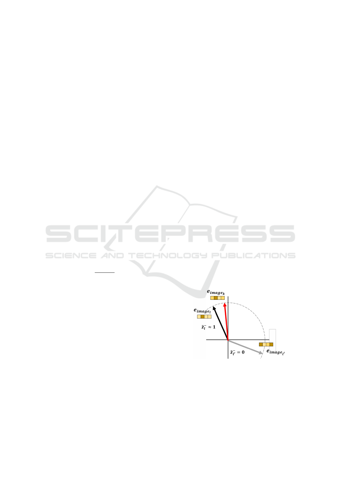
Then, as illustrated in Fig. 2, we estimate for each

image a negative example score ˜z

−

for all unobserved

labels l ∈ L (i.e. when z

= 0):

−

= max

k∈L

l,k

. (8)

This states that the label l can be considered as a

(weak) negative example if its embedding is similar

enough to the embedding of one of the observed la-

bels z

= 1. Negative scores

−

take continuous val-

ues in the range [0, 1] thus giving weak negative labels

for 0 <

−

< 1. The score is 0 if the cosine similarity

value is smaller than the threshold θ (see

−

in Fig. 2).

Figure 2: Estimation of weak negative example scores ˜z

−

and ˜z

−

for unobserved labels and l and l

from the single

observed label k.

Reintroducing the image index n, and recalling the

deﬁnition (4) of the Cross Entropy, our weak negative

A Patch-Based Architecture for Multi-Label Classiﬁcation from Single Positive Annotations

loss function (6) can be rewritten as

∑

) + L

(

−

, 1 −

)

= −

∑

l∈L

n,l

log( ˆy

n,l

) −

∑

l∈L

˜z

−

n,l

log(1 − ˆy

n,l

(9)

This model thus provides negative scores z

−

n,k

which

values depend on the embedding similarity between

unobserved labels z

n,k

= 0 and observed ones z

n,l

= 1.

4 EXPERIMENTS

In this section, we ﬁrst describe the experimental set-

ting in section 4.1. In section 4.2, we validate numer-

ically our proposed architecture and our framework

for negative estimation from multiple image represen-

tations self-similarities. Comparisons and discussions

are ﬁnally provided in section 4.3.

4.1 Settings

4.1.1 Datasets

Only few datasets propose multi-label annotated im-

ages. Datasets traditionally used for detection or

segmentation can nevertheless be adapted to ﬁt the

multi-label learning problem. With such datasets, the

ground truth bounding boxes or masks are discarded,

and only the associated labels are conserved. All the

instances of a label are considered as one label in the

resulting annotation. Hence, in the ground truth an-

notation, y

n,l

= 1 means that at least one instance of

label l is observed in the image x

. In our work, the

single positive label is obtained with a uniform ran-

dom selection between all ground truth labels.

As in (Cole et al., 2021; Verelst et al., 2022), we

consider two datasets that are adapted to the multil-

abel Positive and Unlabeled problem, since different

labels are present in an image: COCO (Lin et al.,

2014) and Pascal VOC (Everingham et al., 2010).

The 2012 version of VOC contains 5,717 images for

model learning and 5,823 images for validation. Ob-

jects can be of 20 different classes, giving 20 different

labels. Each color image can be at a resolution of up

to 640 × 640. The 2014 version of COCO contains

82,081 images for model learning and 40,137 images

for validation. The dataset is annotated with 80 differ-

ent labels. The dataset images are also in colors and

have a resolution of up to 500 × 500.

4.1.2 Model Architecture

The patch extraction was performed on R = 3 down-

sized levels of resolution, with a factor of d = 2 be-

tween each level. The patches are squared sub im-

ages of size w = h = 64, extracted with a stride of 64.

For COCO and VOC, it results in a set of around 130

patches per images. All embeddings e

patch

, e

label

and

image

are of size F = 256. The 64 × 64 patches are

processed with a CNN backbone. This patch embed-

der contains the ﬁrst ﬁve EfﬁcientNet blocks with the

same hyperparameters than (Tan and Le, 2019). The

last two layers are composed of an average pooling

layer and a fully connected layer of size F = 256 in

order to obtain the patch representations e

patch

Label embeddings E

label

of size |L|×F are learned

by the model, the number of labels being |L| = 80

for COCO and |L| = 20 for VOC. Attention pooling

is performed with a regular cross attention and pro-

cessed by a MLP of two layers with 256 neurons,

resulting in L image representations e

image

of size

F = 256. All weights are initialized with the unit vari-

ance scaling method. The GELU activation is used for

MLPs and the swish activation for all convolutions.

The experiments were conducted on one Tesla P40

GPU through an Azure virtual machine. Our model

has been trained for 25 epochs with batches of 16 im-

ages. The starting learning rate is set to lr = 0.001 and

scheduled to decrease every 5 epochs, taking the dif-

ferent values lr = [0.001, 0.0005, 0.00025, 0.000125].

We use the optimizer LAMB (You et al., 2019) with

a weight decay of 0.0001. For the proposed negative

estimation framework, we used θ = 0 to compute the

weight β in (7), resulting in a standard ReLU for the

similarity normalization.

4.1.3 Compared Methods

We consider as reference the model trained using full

supervision (i.e. all positives and negatives labels are

known) with L

BCE

(5). We recall that all other models

are trained using only one positive label per image.

We also compare our method with two closely re-

lated methods (Cole et al., 2021) and (Verelst et al.,

2022) addressing the problem of multi-label learning

with single positive examples. All results are obtained

using the mean average precision (mAP) as the eval-

uation metric on the same validation sets of images

and from models trained on the same dataset versions.

We highlight that (Cole et al., 2021) presents results

obtained with a pre-trained (and ﬁne-tuned) Resnet-

50. Our architecture being trained from scratch, we

consider the setting of (Verelst et al., 2022), obtained

with conditions similar to ours. Hence, for compar-

isons with (Cole et al., 2021), we report the results

VISAPP 2023 - 18th International Conference on Computer Vision Theory and Applications

from (Verelst et al., 2022), where Resnet-50 archi-

tectures are trained from scratch with different losses

during 100 epochs.

We provide comparisons with the models obtained

after 100 epochs with the losses L

, L

EPR

, L

ROLE

proposed in (Cole et al., 2021) and L

EN+CL

, L

EN+SCL

from (Verelst et al., 2022). In brief, L

is the ”as-

sume negative” loss considering all unobserved labels

as negatives; L

EPR

is the expected positive regulariza-

tion applying a penalization to make the sum of pos-

itively predicted labels close to the average number

of positive labels per image; and L

ROLE

is the reg-

ularized online label estimation which considers the

same penalization and also estimates ground truth un-

observed labels as parameters of the model for all im-

ages. Next, L

EN+CL

is the expected negative with con-

sistency loss that uses augmented versions of an im-

age; and L

EN+SCL

is the expected negative with spa-

tial consistency loss that predicts spatial classiﬁcation

scores on an augmented image feature map.

When training our architecture with L

EPR

, the av-

erage label per image is set to k = 2.92 for COCO and

k = 1.38 for VOC. As recommended in (Cole et al.,

2021), for L

ROLE

, lr is multiplied by 10 in the branch

estimating the value of all unobserved labels.

4.2 Results and Comparisons

We now present experiments to validate both the ar-

chitecture and the framework for negative example

estimation. In Table 1, we provide mAP obtained

with our architecture (top part) and the Resnet-50 one

(bottom part). For fair comparison of architectures,

both models have been trained from scratch with the

loss L

BCE

. This provides upper bounds for the archi-

tectures, as this experimental setting corresponds to

the ”ideal” case where all positive and negative are

known. Globally, our patch-based architecture seems

adapted to multiple label learning. In full supervi-

sion, our architecture achieved 65.8 on COCO, which

is better than the 64.8 reported in (Verelst et al., 2022)

for the Resnet-50. On VOC, the difference in favor of

our patch model is signiﬁcant (61.6 vs 53.4).

To validate our negative example estimation

framework, we present results obtained in the sin-

gle positive case. We recall that our strategy con-

sists in using image representations self-similarities

to estimate weak negative examples that are plugged

into the loss L

. As illustrated in Table 1, for the

same number of epochs, mAP results are close to the

ones obtained with full supervision (63.2 vs 65.8 for

COCO and 60.4 vs 61.6 for VOC).

We also trained our patch-based architecture with

the competing L

, L

ROLE

and L

EPR

losses. Our ar-

chitecture trained with our negative estimation propo-

sition gives the best results both on COCO and VOC.

With L

, the sum of predicted labels is always close

to 1, which better ﬁts the VOC dataset (which true

mean number of labels per image is k = 1.38), than

the COCO one (k = 2.92). It should be noticed that

ROLE

underperforms with the considered learning

setting. We suggest this is due to the complexity of

the model, which intends to estimate all unobserved

labels with a dedicated branch in the loss function.

For completeness, we reproduce in Table 1 (bot-

tom part) the mAP results reported in (Verelst et al.,

2022), when training a Resnet-50 architecture from

scratch with the competing losses. Contrary to our

architecture, the decrease of mAP performance with

single positive examples is signiﬁcant with respect to

the full supervision.

All these results indicate that the proposed frame-

work is adapted to the complex multi-label PU prob-

lem including only single positive examples.

4.3 Discussion

4.3.1 Computational Burden

The computational burden for training our patch-

based architecture is signiﬁcantly reduced with re-

spect to the Resnet-50 model of (Cole et al., 2021)

and (Verelst et al., 2022). First, the model size is re-

duced by a factor 100. Our model has approximately

250K parameters to learn, whereas the Resnet-50 ar-

chitecture is composed of 23M parameters. With our

light patch-based architecture, better results are also

obtained with only 25 epochs, instead of 100 epochs

for the Resnet-50 architectures. This suggests that our

architecture generalizes better.

4.3.2 Hyper-Parameters

Our weak negative loss does not include any hyper-

parameter. Excepting the network architecture, the

only extra hyper-parameter of our full model is the

threshold of the cosine similarity in (7) that we sim-

ply ﬁx to θ = 0. On the other hand, the losses L

EPR

and L

ROLE

penalize the sum of positive predictions

with respect to the average number of label per image.

This is a strong assumption, as the variance of posi-

tive labels on all image of the dataset can be large.

Moreover, the prior knowledge of the mean number

of labels is often not available in real use cases.

The loss L

ROLE

also relies on an online estimation

of all unobserved ground truth annotations from cur-

rent predictions. This model is thus greatly inﬂuenced

by the initialization and the ﬁrst few epochs, while in-

creasing the memory requirements.

A Patch-Based Architecture for Multi-Label Classiﬁcation from Single Positive Annotations

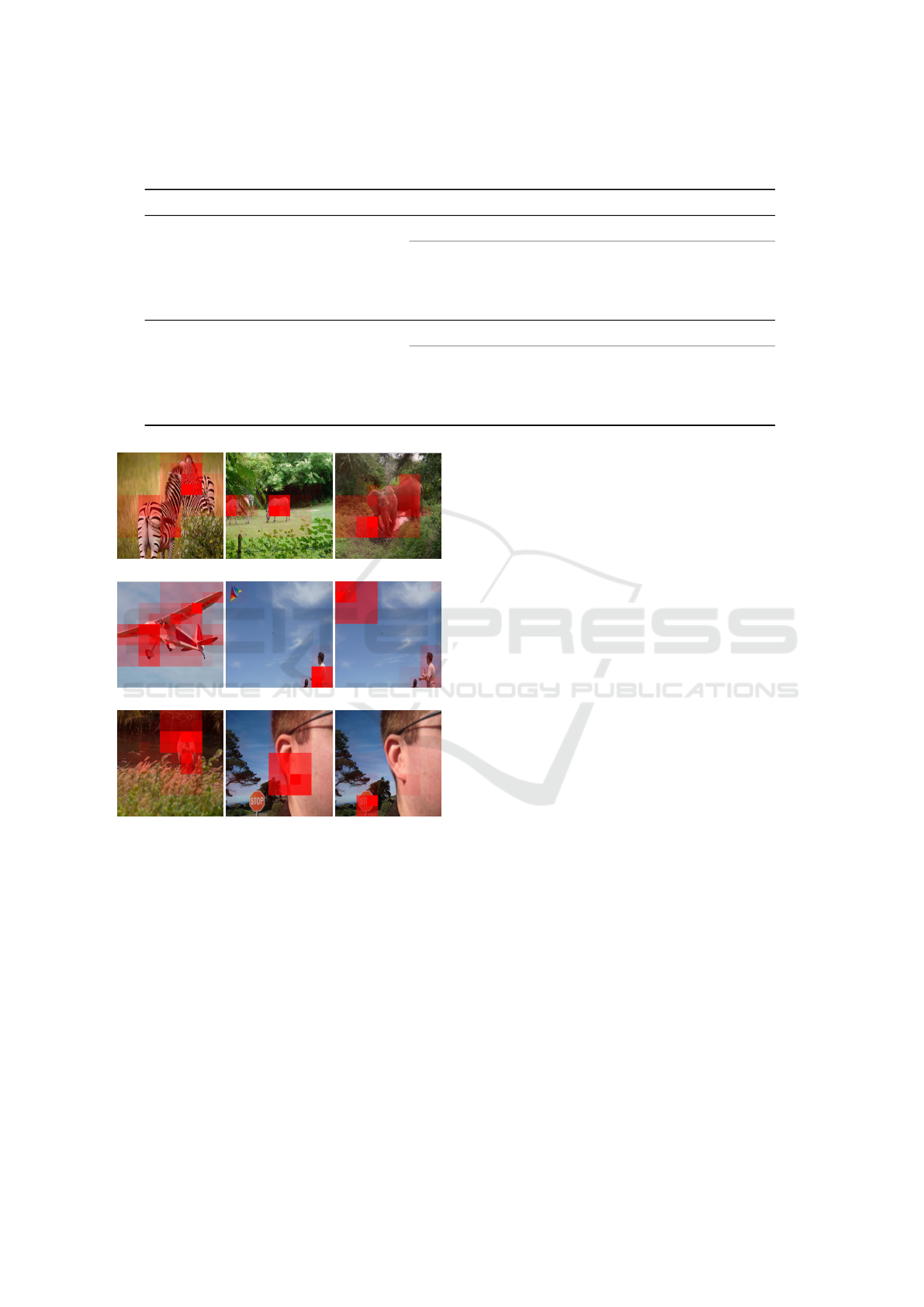
Table 1: mAP results for our patch approach trained for 25 epochs and different losses (top) and comparisons (bottom) with

the results reported by (Verelst et al., 2022) after training a Resnet-50 architecture for 100 epochs. Best results in bold.

Model Loss/method COCO-14 VOC-12

Patch based

architecture

(ours)

BCE

(fully-annotated) 65.8 61.6

(Cole et al., 2021) 62.6 60.0

EPR

(Cole et al., 2021) 61.4 58.8

ROLE

(Cole et al., 2021) 33.3 49.7

(ours) 63.2 60.4

Resnet-50

(reported in (Verelst et al., 2022))

BCE

(fully-annotated) 64.8 53.4

(Cole et al., 2021) 50.2 45.7

ROLE

(Cole et al., 2021) 51.9 45.0

EN+CL

(Verelst et al., 2022) 54.3 47.0

EN+SCL

(Verelst et al., 2022) 54.0 50.4

zebra: 94.8 zebra: 98.9 elephant: 58.6

airplane: 77.5 person: 51.1 kite: 55.5

bear: 57.1 person: 34.2 stop sign: 96.6

Figure 3: Examples of patch attention scores for true pos-

itives. Patches are ﬁlled with their attention score values,

that vary from 0 (transparent) to 1 (red). The second line

present the prediction score for the given labels..

4.3.3 Label Localization

Our architecture has the potential to locate patch ex-

amples corresponding to a detected label (Fig. 3). In-

deed, the attention scores α

l,i

computed in the atten-

tion patch pooling with relation (1) (see block 4 of

Fig. 1) allows determining the level of patch i par-

ticipation to the classiﬁcation decision relative to la-

bel l. The patch-based model thus offers a natural

framework to interpret the obtained results, without

relying on advanced gradient backpropagation mech-

anisms (Selvaraju et al., 2017).

4.3.4 Pre-Training and Fine-Tuning

It is important to underline the current limitation of

our approach with respect to Resnet-50 architectures.

The models (Cole et al., 2021) and (Verelst et al.,

2022) provide signiﬁcant better mAP results (72 for

COCO and even 88 for VOC), when considering

a Resnet-50 pre-trained on Imagenet, with potential

ﬁne-tuning reﬁnements. We postulate that our results

could also be improved by pretraining either our full

patch-based architecture on Imagenet, or the patch

embedder on bounding boxes of a detection dataset.

The performance could also be increased by conduct-

ing an extensive hyper-parameter search (dimension

of the representation space F, number of attention

layers, ...) and training tuning.

5 CONCLUSION

In this work, we proposed a light patch-based archi-

tecture for multi-label classiﬁcation problems. Lever-

aging on patch embedding self-similarities, we pro-

vide a strategy for estimating negative examples when

facing the challenging problem of positive and un-

labeled learning. The patch-based attention strategy

also gives a natural framework to localize detected la-

bels within images.

Numerical experiments demonstrate the interest

of the approach when no dedicated pre-trained net-

work is available. Our model is able to generalize fast

from few labels, as it provides relevant results when

trained from scratch during a few epochs. In the re-

lated literature, the best performances are obtained

with pre-trained Resnet-50 architectures having a

number of parameters 100 times greater than ours.

VISAPP 2023 - 18th International Conference on Computer Vision Theory and Applications

In order to improve our model and reach state-of-

the-art results, the main directions we draw are the

online estimation of positive and negative example at

batch level, the pre-training of the patch embedder

and an improved model to cluster the patch embed-

ding space with respect to the labels.

REFERENCES

Bekker, J. and Davis, J. (2020). Learning from positive

and unlabeled data: A survey. Machine Learning,

109(4):719–760.

Buades, A., Coll, B., and Morel, J.-M. (2005). A non-local

algorithm for image denoising. In IEEE/CVF Conf. on

Computer Vision and Pattern Recognition, volume 2,

pages 60–65 vol. 2.

Carbonneau, M.-A., Cheplygina, V., Granger, E., and

Gagnon, G. (2018). Multiple instance learning: A sur-

vey of problem characteristics and applications. Pat-

tern Recognition, 77:329–353.

Chen, C.-F. R., Fan, Q., and Panda, R. (2021). Crossvit:

Cross-attention multi-scale vision transformer for im-

age classiﬁcation. In IEEE Int. Conf. on Computer

Vision, pages 357–366.

Cole, E., Mac Aodha, O., Lorieul, T., Perona, P., Morris, D.,

and Jojic, N. (2021). Multi-label learning from single

positive labels. In IEEE/CVF Conf. on Computer Vi-

sion and Pattern Recognition, pages 933–942.

Coup

e, P., Manj

on, J. V., Fonov, V., Pruessner, J., Robles,

M., and Collins, D. L. (2011). Patch-based segmenta-

tion using expert priors: Application to hippocampus

and ventricle segmentation. NeuroImage, 54(2):940–

954.

Dosovitskiy, A., Beyer, L., Kolesnikov, A., Weissenborn,

D., Zhai, X., Unterthiner, T., Dehghani, M., Minderer,

M., Heigold, G., Gelly, S., et al. (2020). An image is

worth 16x16 words: Transformers for image recogni-

tion at scale. arXiv preprint arXiv:2010.11929.

Efros, A. A. and Leung, T. K. (1999). Texture synthesis

by non-parametric sampling. In IEEE Int. Conf. on

Computer Vision, volume 2, pages 1033–1038.

Everingham, M., Van Gool, L., Williams, C. K., Winn, J.,

and Zisserman, A. (2010). The pascal visual object

classes (voc) challenge. International journal of com-

puter vision, 88(2):303–338.

Freeman, W. T., Jones, T. R., and Pasztor, E. C. (2002).

Example-based super-resolution. IEEE Computer

Graphics and Applications, 22(2):56–65.

He, K., Gkioxari, G., Doll

ar, P., and Girshick, R. (2017).

Mask r-cnn. In IEEE Int. Conf. on Computer Vision,

pages 2961–2969.

Huang, X. and Yan, M. (2018). Nonconvex penalties with

analytical solutions for one-bit compressive sensing.

Signal Processing, 144:341–351.

Ilse, M., Tomczak, J., and Welling, M. (2018). Attention-

based deep multiple instance learning. In Int. Conf. on

Machine Learning, pages 2127–2136.

Ishida, T., Niu, G., Hu, W., and Sugiyama, M. (2017).

Learning from complementary labels. Advances in

neural information processing systems, 30.

Jaegle, A., Gimeno, F., Brock, A., Vinyals, O., Zisserman,

A., and Carreira, J. (2021). Perceiver: General percep-

tion with iterative attention. In Int. Conf. on Machine

Learning, pages 4651–4664.

Kanehira, A. and Harada, T. (2016). Multi-label ranking

from positive and unlabeled data. In IEEE/CVF Conf.

on Computer Vision and Pattern Recognition, pages

5138–5146.

Lanchantin, J., Wang, T., Ordonez, V., and Qi, Y. (2021).

General multi-label image classiﬁcation with trans-

formers. In IEEE/CVF Conf. on Computer Vision and

Pattern Recognition, pages 16478–16488.

Lin, M., Chen, Q., and Yan, S. (2013). Network in network.

arXiv preprint arXiv:1312.4400.

Lin, T.-Y., Maire, M., Belongie, S., Hays, J., Perona, P.,

Ramanan, D., Doll

ar, P., and Zitnick, C. L. (2014).

Microsoft coco: Common objects in context. In Euro-

pean Conf. on Computer Vision, pages 740–755.

Liu, L., Chen, J., Fieguth, P., Zhao, G., Chellappa, R.,

and Pietik

ainen, M. (2019). From bow to cnn: Two

decades of texture representation for texture classi-

ﬁcation. International Journal of Computer Vision,

127(1):74–109.

Mac Aodha, O., Cole, E., and Perona, P. (2019). Presence-

only geographical priors for ﬁne-grained image classi-

ﬁcation. In IEEE Int. Conf. on Computer Vision, pages

9596–9606.

Read, J., Pfahringer, B., Holmes, G., and Frank, E. (2009).

Classiﬁer chains for multi-label classiﬁcation. In Joint

European conference on machine learning and knowl-

edge discovery in databases, pages 254–269.

Redmon, J., Divvala, S., Girshick, R., and Farhadi, A.

(2016). You only look once: Uniﬁed, real-time object

detection. In IEEE/CVF Conf. on Computer Vision

and Pattern Recognition, pages 779–788.

Ren, S., He, K., Girshick, R., and Sun, J. (2015). Faster

r-cnn: Towards real-time object detection with region

proposal networks. Advances in neural information

processing systems, 28.

Selvaraju, R. R., Cogswell, M., Das, A., Vedantam, R.,

Parikh, D., and Batra, D. (2017). Grad-cam: Visual

explanations from deep networks via gradient-based

localization. In IEEE Int. Conf. on Computer Vision,

pages 618–626.

Tan, M. and Le, Q. (2019). Efﬁcientnet: Rethinking model

scaling for convolutional neural networks. In Int.

Conf. on Machine Learning, pages 6105–6114.

Trockman, A. and Kolter, J. Z. (2022). Patches are all you

need? arXiv preprint arXiv:2201.09792.

Varma, M. and Zisserman, A. (2008). A statistical ap-

proach to material classiﬁcation using image patch ex-

emplars. IEEE Trans. on Pattern Analysis and Ma-

chine Intelligence, 31(11):2032–2047.

Vaswani, A., Shazeer, N., Parmar, N., Uszkoreit, J., Jones,

L., Gomez, A. N., Kaiser, Ł., and Polosukhin, I.

(2017). Attention is all you need. Advances in Neural

Information Processing Systems, 30.

A Patch-Based Architecture for Multi-Label Classiﬁcation from Single Positive Annotations

Verelst, T., Rubenstein, P. K., Eichner, M., Tuytelaars, T.,

and Berman, M. (2022). Spatial consistency loss for

training multi-label classiﬁers from single-label anno-

tations. arXiv preprint arXiv:2203.06127.

Wei, Y., Xia, W., Huang, J., Ni, B., Dong, J., Zhao, Y., and

Yan, S. (2014). Cnn: Single-label to multi-label. arXiv

preprint arXiv:1406.5726.

Xiao, T., Singh, M., Mintun, E., Darrell, T., Doll

ar, P., and

Girshick, R. (2021). Early convolutions help trans-

formers see better. Advances in Neural Information

Processing Systems, 34:30392–30400.

You, Y., Li, J., Reddi, S., Hseu, J., Kumar, S., Bhojana-

palli, S., Song, X., Demmel, J., Keutzer, K., and

Hsieh, C.-J. (2019). Large batch optimization for deep

learning: Training bert in 76 minutes. arXiv preprint

arXiv:1904.00962.

Zaheer, M., Kottur, S., Ravanbakhsh, S., Poczos, B.,

Salakhutdinov, R. R., and Smola, A. J. (2017). Deep

sets. Advances in Neural Information Processing Sys-

tems, 30.

Zhang, D., Zhang, H., Tang, J., Wang, M., Hua, X., and

Sun, Q. (2020). Feature pyramid transformer. In Eu-

ropean Conf. on Computer Vision, pages 323–339.

Zhao, T., Zhang, N., Ning, X., Wang, H., Yi, L., and Wang,

Y. (2022). Codedvtr: Codebook-based sparse voxel

transformer with geometric guidance. In IEEE/CVF

Conf. on Computer Vision and Pattern Recognition,

pages 1435–1444.

VISAPP 2023 - 18th International Conference on Computer Vision Theory and Applications