Deep W-Networks: Solving Multi-Objective Optimisation Problems with

Deep Reinforcement Learning

Jernej Hribar, Luke Hackett and Ivana Dusparic

School of Computer Science and Statistics, Trinity College Dublin, Ireland

Keywords:

Deep Reinforcement Learning, Deep Q-Networks, W-Learning, Deep W-Networks, and Multi-Objective.

Abstract:

In this paper, we build on advances introduced by the Deep Q-Networks (DQN) approach to extend the multi-

objective tabular Reinforcement Learning (RL) algorithm W-learning to large state spaces. W-learning algo-

rithm can naturally solve the competition between multiple single policies in multi-objective environments.

However, the tabular version does not scale well to environments with large state spaces. To address this

issue, we replace underlying Q-tables with DQN, and propose an addition of W-Networks, as a replacement

for tabular weights (W) representations. We evaluate the resulting Deep W-Networks (DWN) approach in

two widely-accepted multi-objective RL benchmarks: deep sea treasure and multi-objective mountain car. We

show that DWN solves the competition between multiple policies while outperforming the baseline in the form

of a DQN solution. Additionally, we demonstrate that the proposed algorithm can ﬁnd the Pareto front in both

tested environments.

1 INTRODUCTION

Many real world problems such as radio resource

management (Giupponi et al., 2005), infectious dis-

ease control (Wan et al., 2020), energy-balancing in

sensor networks (Hribar et al., 2022), etc., can be for-

mulated as a multi-objective optimisation problem.

Whenever an agent is tackling such a problem in a

dynamic environment, a single objective Reinforce-

ment Learning (RL) methods such as Q-learning will

not result in a behaviour that will be optimal for all

objectives. Instead, the single objective solution will

most likely prefer one objective over others. Al-

ternatively, the agent can employ a Multi-Objective

Reinforcement Learning (MORL) method. Unfortu-

nately, while much work has been completed in tabu-

lar MORL (Liu et al., 2015), the curse of dimension-

ality limits the applicability of these methods to real-

world problems. The curse of dimensionality refers to

the challenges that come with organizing and analyz-

ing data that has an intractably and/or inﬁnitely large

state-space, for example, using images as input states.

Recent developments in RL merged Q-Learning with

Neural Networks (Mnih et al., 2013), vastly expand-

ing the complexity of problems that could be tackled

with RL. Work has been done in the past few years in

order to employ Deep Q-Networkss (DQNs) to solve

Multi-Objective problems (Liu et al., 2015). How-

ever, most of the proposed solutions have drawbacks.

These drawbacks range from a required high number

of sampled experiences to train the neural networks,

which will take an extended amount of time, to adding

complexity by creating new types of networks with

altered memory storage. To overcome these obsta-

cles, in this paper, we propose a deep learning ex-

tension to a tabular multi-objective technique called

W-learning (Humphrys, 1995).

W-Learning was ﬁrst proposed in the late

90’s (Humphrys, 1995), as a multi-policy way to solve

multi-Objective problems that use Q-Learning agents

with a single objective as part of a larger system. The

main principle is that there will be many Q-Learning

agents, each with a different policy. These agents

will all suggest an action that will be selﬁsh, and the

best action will need to be determined from these sug-

gested selﬁsh actions. The goal of W-Learning is to

determine which of these actions should be selected,

ensuring the right agent “wins”. The way it deter-

mines this is by attempting to ﬁgure out how much

the agent cares about the action that it suggests. Some

scenarios or states might not impact the reward of cer-

tain agents so much however it may massively im-

pact one or some of them. W-learning has been suc-

cessfully applied in a range multi-objective problems,

from speed limit control on highways (Kusic et al.,

2021), smart grid (Dusparic et al., 2015), and con-

Hribar, J., Hackett, L. and Dusparic, I.

Deep W-Networks: Solving Multi-Objective Optimisation Problems with Deep Reinforcement Lear ning.

DOI: 10.5220/0011610300003393

In Proceedings of the 15th International Conference on Agents and Artiﬁcial Intelligence (ICAART 2023) - Volume 2, pages 17-26

ISBN: 978-989-758-623-1; ISSN: 2184-433X

 2023 by SCITEPRESS – Science and Technology Publications, Lda. Under CC license (CC BY-NC-ND 4.0)

ﬂict detection in self-adaptive systems (Cardozo and

Dusparic, 2020). However, as W-learning was pro-

posed long before deep learning was successfully im-

plemented in RL to deal with the curse of dimen-

sionality (Mnih et al., 2013), this limited the domains

and scale of problems that W-Learning can be applied

to. In this paper, we take advantage of advances in-

troduced by DQN to train multiple Artiﬁcial Neural

Network (ANN) on different objectives and propose

a new “deep” variant of W-Learning to address com-

petition between these objectives.

One of the most signiﬁcant advantages of multi-

policy algorithms over single-policy, e.g., Q-learning,

is in their ability to ﬁnd the Pareto Optimal be-

haviour(Jin and Sendhoff, 2008). To be Pareto Op-

timal, the agent’s actions must be such that an im-

provement in its decision process for an objective will

not harm the reward for any other objective. Single-

policy algorithms rely on some speciﬁcation of pref-

erences for given objectives and, therefore, will not

necessarily ﬁnd the policy that will result in the opti-

mal Pareto front. In other words, multi-objective al-

gorithms require less information about the environ-

ment before training and are generally more favoured

for use in ofﬂine learning.

Our proposed Deep W-Networks (DWN) algo-

rithm takes advantage of the computational efﬁciency

of single-policy algorithms by considering each ob-

jective separately. These policies will suggest a self-

ish action that will only maximise their own reward.

However, the DWN resolves the competition be-

tween greedy single-objective policies by relying on

W-values representing policies’ value to the system.

These W-values can be learned with interaction with

the environment, following logical steps similar to a

well-known Q-learning algorithm. In our proposed

implementation, we employ two DQNs for each ob-

jective. One DQN is used to learn a greedy policy

for the given objective, while the second DQN has

only one output representing the policy’s W-value for

a given state input. Furthermore, DWN has the ben-

eﬁt of training all policies simultaneously, which al-

lows for a faster learning process. Additionally, DWN

can take advantage of modularity, meaning that poli-

cies can be trained separately and then included in the

DWN agent. Modularity also enables policies to be

altered, e.g., the reward function is changed, added,

or deactivated, without the need to re-train all other

policies.

The rest of the paper is organised as follows. In

the next section, we discuss the most important de-

sign features of Deep Reinforcement Learning (DRL)

introduced in the last decade and related work. In sec-

tion 3 we present and describe our proposed DWN al-

gorithm. Followed by evaluation section 4, in which

we employ two multi-objective environments: multi-

objective mountain car and deep sea treasure. We

show in both environments that DWN is capable of

resolving the competition between multiple policies

while outperforming the baseline in the form of DQN

solution. Finally, we provide concluding remarks in

section 5.

2 BACKGROUND

In this section, we introduce the essential elements

required to understand DRL and review related algo-

rithms capable of resolving multi-objective problems.

2.1 Deep Reinforcement Learning

The goal of RL algorithm is to ﬁnd the optimal policy

∗

for an environment that is fully characterised with

an Markov Decision Process (MDP) (LeCun et al.,

2015). With MDP we describe a sequential decision-

making process in a form of a state-space S , an action

space A, a reward function R, and a set of transition

probabilities between the states P . In such settings,

the optimal policy π

∗

is the policy that will maximise

the long-term reward.

An example of a DRL algorithm that revolu-

tionised the ﬁeld in 2013 is DQN. The DQN algo-

rithm is a deep learning extension of a well-known

action-value algorithm named Q-learning. In action-

value based methods, the agent interacts with the en-

vironment by taking actions a and receiving a reward

r that indicates if the taken action was desirable or

not. The Q represents the quality of an action-value

Q(s,a), with s representing the state. The objective

of the RL algorithm is to accurately estimate Q val-

ues for all action-values using a Bellman equation.

Once the agent can accurately determine all values,

it can ﬁnd the optimal policy π

∗

for selection actions

that will maximise the expected reward r + γQ(s

with γ representing the discount for rewards obtained

in next time-step. The Q-values are updated in itera-

tions as follows:

(s,a) = E

s∼S



r = γ max Q

∗

)|s,a



; (1)

and converge to the optimal value when:

→ Q

∗

as i → ∞. (2)

However, such an iterative approach requires the

agent to explore the entire state space, i.e., try all pos-

sible action in every state. In practice, such an ap-

proach is impossible as such exploration would take a

ICAART 2023 - 15th International Conference on Agents and Artiﬁcial Intelligence

gargantuan amount of time and computational power.

Instead, a state-space approximator is used. An exam-

ple of a very effective non-linear state-space approxi-

mator is ANN.

In the DQN, a ANN function approximator with

weights θ is employed to represent Q-network. The

agent uses the network to estimate the action-values,

i.e., Q(s,a;θ) ≈ Q

∗

(s,a). The values in the ANN are

updated, i.e., trained, at each iteration i by minimising

the loss:

(θ

) = E

s,a∼ρ(·);s

∼S



− Q(s,a;θ

))



, (3)

where y

= E

s∼S

[r + γmax

Q(s

;θ

i−1

|s,a] repre-

sent target and ρ is the probability distribution over

sequences. Note that when determining the target, the

values from the previous iteration, i.e., θ

i−1

, are held

ﬁxed. The gradient of the loss function is then deter-

mined as:

∇

(θ

) = E

s,a∼ρ(·);s

∼S



r +γmax

Q(s

;θ

i−1

−

Q(s,a)



∇

Q(s,a;Q

)



. (4)

In practice, the loss function is optimised using gra-

dient descent as it is less computation-intensive than

computing the expectation E directly. However, the

training process can be unstable and prone to con-

verge to a local optimum. To remedy this issue, the

DQN introduced experience replay and the use of pol-

icy and target ANN.

Experience replay is a batch memory M into

which the agent is storing experiences. An experience

typically consist of a state, the next state, selected ac-

tion, and obtained reward, i.e., a tuple < s,a,s

,r >.

The agent often samples experiences uniformly ran-

domly during the training process. However, be-

cause not all experiences are equal in terms of im-

portance to the learning process, a much better ap-

proach is to prioritise them, i.e., increase the proba-

bility of their selection. Using Prioritised Experience

Replay (PER)(Schaul et al., 2015) we determine the

probability of sampling an experience i as:

P(i) =

∑

, (5)

with factor ζ,ζ ∈ [0, 1] controlling the degree to which

experiences are prioritised. Using PER can signiﬁ-

cantly reduce the time the agent requires to ﬁnd the

optimal policy. To further stabilise the learning pro-

cess, the DQN algorithm introduced the use of tar-

get ANN for estimating the Q(s

) during training.

Such an approach is necessary because using the same

ANN for determining both Q-values can results in

very similar estimations due to possible small differ-

ence in s and s

. Therefore, using a target policy for

Q(s

) estimation can prevent such occurrences.

In our work, we adopt these aforementioned ad-

vances to extend the original W-learning algorithm

usability in large state spaces.

2.2 Multi-Objective Reinforcement

Learning

Existing RL methods employed for resolving multi-

objective optimisation problems can be generalised

into two groups: tabular RL and DRL methods.

An example of a tabular methods are GM-Sarsa(0)

(Sprague and Ballard, 2003) and its extension with

weighted sum approach (Karlsson, 1997). GM-

Sarsa(0) (Sprague and Ballard, 2003) aims to ﬁnd

good policies concerning the composite tasks as op-

posed to ﬁnding the best policy for each task and then

merging these into a single policy. On the other hand,

the authors in (Karlsson, 1997) proposed to use a syn-

thetic objective function to emphasise the importance

of each objective in the form of weight for Q-values.

Unfortunately, neither of these methods performs well

in ﬁnding the optimal multi-objective policy. Addi-

tionally, the performance of the tabular methods dete-

riorates when applied in environments with large state

spaces.

The second group, DRL methods (Mossalam

et al., 2016; Nguyen et al., 2020; Tajmajer, 2018;

Abels et al., 2019), can deal with large state

spaces. The deep optimistic linear support learn-

ing (Mossalam et al., 2016) is an example of the ﬁrst

known extension of the DQN that dealt with multi-

objectivity. The limitation of linear support approach

is in redundant computations and additional required

representations. Both limitations can be overcome in

two-stage multi-objective DRL (Nguyen et al., 2020)

approach. In the latter, once policies are learned,

policy-independent parameters are tuned using a sep-

arate algorithm that attempts to estimate the Pareto

frontier of the system. Similarly, modular multi-

objective DRL with subsumption architecture (Taj-

majer, 2018) was proposed that combines the results

of single policies, represented by a DQN, to take the

action most amenable to all rewards for each envi-

ronment step. The approach resembles a voting sys-

tem with Q-values representing a vote for a certain

policy. Finally, dynamic weights in multi-objective

DRL (Abels et al., 2019) were proposed to deal with

situations where the relative importance of weights

changes during training. In contrast, our proposed

DWN has the beneﬁt of simultaneously training all

Deep W-Networks: Solving Multi-Objective Optimisation Problems with Deep Reinforcement Learning

policies, which allows for a faster dynamic adjust-

ment of policy rewards that the above DRLs methods

lack.

3 DEEP W-LEARNING

FRAMEWORK

In this section, we detail out our proposed multi-

objective DWN approach. We denote the multi-

objective environment with tuple < N,S ,A,R , Π >

in which N is the number of policies, S represents

the state space, A is the set of all available actions,

R = {R

,...,R

} is set of reward functions, and Π =

π,...,π

denotes the set of available policies. At

each decision epoch t policies observe the same state

s(t) ∈ S and every policy suggest an action. The

agent’s objective is to select the best possible action

from the vector of actions nominated by agents for

execution at that time-step a(t) = {a

(t),..., a

(t)}.

Furthermore, we denote the selected action at time-

step t with index j, i.e., the selected action is denoted

as a

(t). Additionally, within our environment, we

use Π

− j

to denote the set containing all polices ex-

cept the j-th one.

The agent making the decision in a multi-objective

environment at each time-step has to determine to

what extent it will take into account each of the ob-

jectives. In other words, the agent has to continuously

keep resolving the competition between multiple ob-

jectives. In W-learning, each objective is represented

with a single Q-learning policy; each Q-learning pol-

icy has a different goal and, depending on the ob-

served state s(t), suggests a greedy action a

(t). These

actions are often conﬂicting with each other, and to

resolve the competition, the agent learns a table of

weights for each state, called the W-values. For each

observed state s(t), the agent obtains W

(t) where i is

the index of the policy. The agent then takes the ac-

tion suggested by the policy associated with the high-

est W

(t):

(t) = max ({W

(t),...,W

(t)}). (6)

Note that the index j marks the W-value of the policy

the agent has selected. Updating the W-values fol-

lows a very similar formulation as updating the Q-

values(Eq.1):

(t) ← (1 − α)W

(t) + α



Q(s(t),a

(t)) − (R

(t)+

γ max

(t+1)∈A

Q(s(t + 1), a

(t + 1))



. (7)

However, the agent will not update the W-value of the

selected policy, i.e., the agent only updates W-values

for set of policies Π

− j

. Excluding W-Learning update

for the selected policy allows other policies to emerge

as the leader overtime. Such an approach is accept-

able in practice as polices become more adept at their

given task. Additionally, the updating constraint only

applies for W-values, the agent will update Q-values

for every policy, i.e., for the set Π.

Algorithm 1: Deep W-Learning with PER.

1: Input: Minibatch size K, replay memory size M,

exploration rates ε

, ε

, smoothing factor ζ, ex-

ponent β, w-learning learning rate α, soft update

factors τ

, τ

2: Initialize N Q-networks θ

, target

, and replay

memory D

∀i ∈ {1,. ..,N}

3: Initialize N W-networks θ

, target

, and re-

play memory D

∀i ∈ {1,. ..,N}

4: for t = 0 to T − 1 do

5: Observe s(t),s(t) ∈ S

6: // Nominate actions using epsilon-greedy

approach (ε

)

7: Get a(t) = {a

(t),..., a

(t)}

8: Get W

(t)∀i ∈ {1, .. .,N}

9: // Select and execute action using

epsilon-greedy approach (ε

)

10: Get j-th policy with the highest W-value

using Eq. 6

11: Execute action a

(t), and observe

state s(t + 1)

12: Initiate policy training with Alg. 2

13: Initiate W training with Alg. 3

14: end for

In our proposed DWN implementation, each pol-

icy has two DQN networks. The role of the ﬁrst DQN

is to determine Q-values for the given policy, i.e., for

greedy actions the policy will suggest. On the other

hand, the second DQN has only one output, repre-

senting the W-value, and replaces a tabular represen-

tation of state-W-value pairs present in the original

W-learning implementation. We summarise the pro-

posed DWN in Alg. 1. Each policy requires two re-

play memories, one for Q-networks and another for

the W-networks. Such a split is necessary because the

agent will store a W-learning experience only when

the agent did not select the policy. Additionally, we

employed PER (Schaul et al., 2015) in our implemen-

tation to expedite the learning process.

The most signiﬁcant aspect of the proposed DWN

algorithm is the action-nomination step. In the action

nomination step, each policy suggests a greedy action

with an epsilon probability that it will select a ran-

dom action. Similarly, the agent will select the policy

with the highest W-value but with epsilon probability,

ICAART 2023 - 15th International Conference on Agents and Artiﬁcial Intelligence

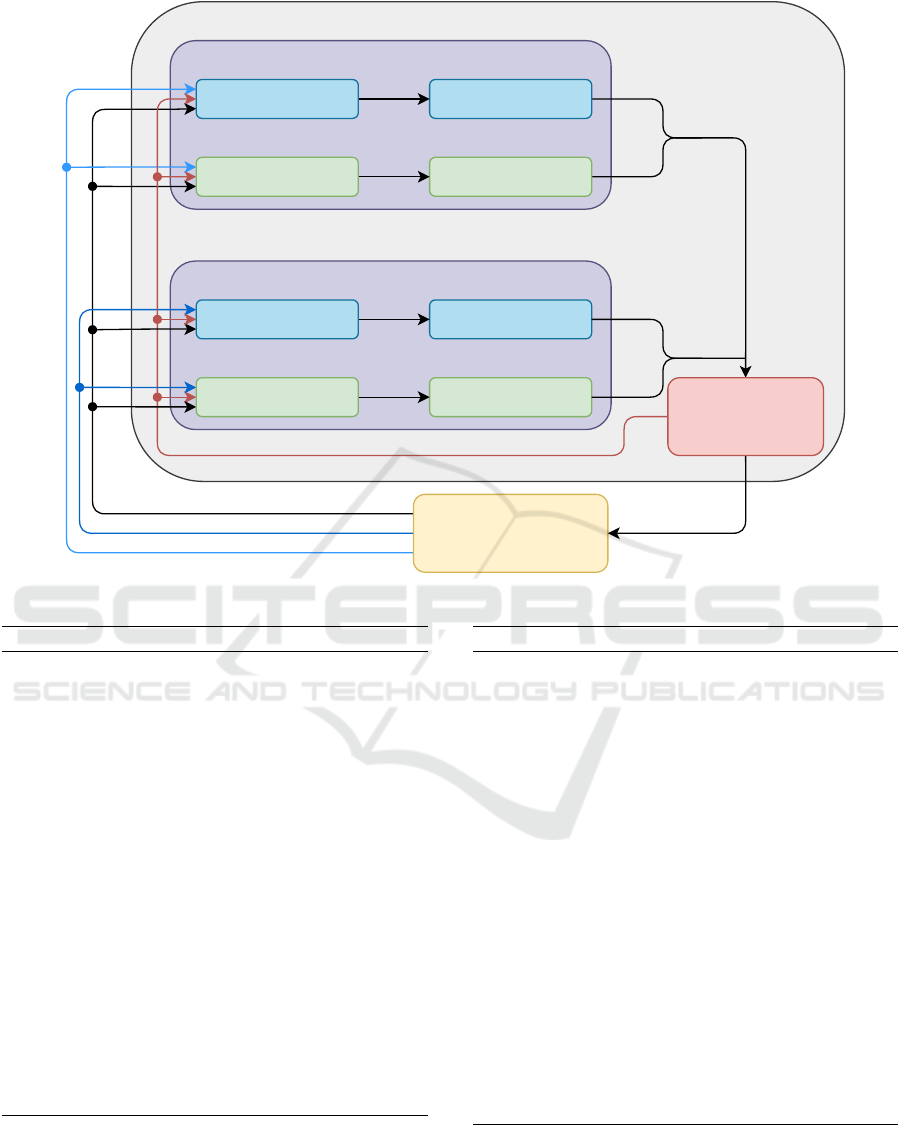
Deep W-Networks Agent

Environment

Q-Policy

W-Values

Policy 1

Q Memory

W Memory

Select the action of the

policy with the highest

W-value

Policy

Training

W Training

Q-Policy

W-Values

Policy N

Q Memory

W Memory

Policy

Training

W Training

State

Reward for Policy N

Reward for Policy 1

Q-values

W-value

Action

Selected Policy and Action

Figure 1: Deep W-Networks architecture.

Algorithm 2: Policy Training.

1: Input:Π, D

,i ∈ {1,...,N}, K, M, ζ, β, θ

,i ∈

{1,...,N},

,i ∈ {1,...,N}

2: for each π

in Π do

3: Determine reward r

(t) using function R

4: Store experience (s(t),a

(t),r

(t),s(t + 1)

in D

with priority p

= max

m<t

5: for each k = 1 to K do

6: Sample transition k ∼ P(k) = p

∑

7: Compute importance-sampling weight:

= (MP( j))

−β

/max

8: Update transition priority p

← |δ

9: Accumulate weight-change:

∆ ← ∆ +ω

·δ

·∇

Q(s(k − 1),a

(k − 1)

10: end for

11: Update weights θ

← θ

+ η · ∆, reset ∆ = 0

12: Soft update target network:

← τ

+ (1 − τ

)

13: Update ε

using decay

14: end for

it might decide to explore, i.e., select the policy ran-

domly. W-values exploration is necessary to avoid a

single policy prevailing at the start of the learning due

to high randomly initialized values and batch learn-

Algorithm 3: W Training.

1: Input:Π, D

,i ∈ {1, ...,N}, K, M, ζ, β, θ

,i ∈

{1,...,N},

,i ∈ {1,...,N}

2: for each π

in Π

− j

3: Determine reward r

(t) using function R

4: Store experience (s(t),a

(t),r

(t),s(t + 1)

in D

with priority p

= max

m<t

5: end for

6: for each π

in Π do

7: for each k = 1 to K do

8: Sample transition k ∼ P(k) = p

∑

9: Compute importance-sampling weight:

= (MP( j))

−β

/max

10: Update transition priority p

← |δ

11: Accumulate weight-change ∆ using Eq. 7

12: end for

13: Update weights θ

← θ

+ η · ∆, reset ∆ = 0

14: Soft update target network:

← τ

+ (1 − τ

)

15: Update ε

using decay

16: end for

ing. Before the learning process can start, the agent

requires a minimum of K experiences stored in the

replay memory to start the training process.

We summarise the steps to train the policy and W-

Deep W-Networks: Solving Multi-Objective Optimisation Problems with Deep Reinforcement Learning

networks in two algorithms and give an overview of

the DWN architecture in Fig. 1. During policy train-

ing (Alg. 2), each policy network optimises for the

highest reward for its target. Note that this process re-

mains unchanged from the original DQN implemen-

tation, but is an integral part of the proposed DWN.

After Q networks have been through a few updates the

W training (Alg. 3) can begin. We achieve the delay

by keeping the batch size for both policy and W train-

ing the same, or greater. The W policy saves the expe-

rience only when it was not selected. In Alg. 3, line 3

we save the W experiences of all policies but j-th,

which was selected (in line 10, Alg. 1). Consequently,

we achieve the delay in training the W networks. Ep-

silon greedy approach of selecting W-values ensures

that the agent does not select the same W network in

every step at the start of the training. In the next sec-

tion, we demonstrate how DWN performs in a multi-

objective environment.

4 EVALUATION

In this section, we evaluate

the proposed DWN using

two multi-objective environments: multi-objective

mountain car and deep sea treasure. The state space

in the ﬁrst environment is hand-crafted and is repre-

sented by only a two-input state vector. The two in-

puts are the car’s position and velocity. The simpliﬁed

case enables us to analyse DWN performance in more

detail. On the other hand, in the second environment,

the deep sea treasure, we use visual inputs as states

to demonstrate that DWN performs well in environ-

ments with large state spaces.

4.1 Multi-Objective Mountain Car

The ﬁrst environment, called Multi-Objective Moun-

tain Car presents a scenario where a car is stuck in the

middle of a valley. The car must reach the top of the

valley. However, the car does not have enough power

to reach the top by driving directly forward. Instead,

the agent has to learn to ﬁrst move away from its ob-

jective, by reversing up the hill to gain momentum,

in order to reach it. We use the environment, with

minor modiﬁcations, as deﬁned in (Vamplew et al.,

2011). The only alteration we made is the maximal

number of steps allowed in an episode. We set the

limit to 2000 because the goal of analysis in this en-

vironment is to gain a deeper understanding of DWN

performance.

DWN algorithm implementation and evaluation code

is available on github.com/deepwlearning/deepwnetworks.

250 500 750 1000 1250 1500 1750 2000 2250

110

250

500

750

1,000

1,250

1,500

1,750

Episode number

Average number of steps needed to reach the top (over 10 episodes)

DQN

DWN

Pareto

250 500 750 1000 1250 1500 1750 2000 2250

110

250

500

750

1,000

1,250

1,500

1,750

Episode number

Average number of steps needed to reach the top (over 10 episodes)

DQN

DWN

Pareto

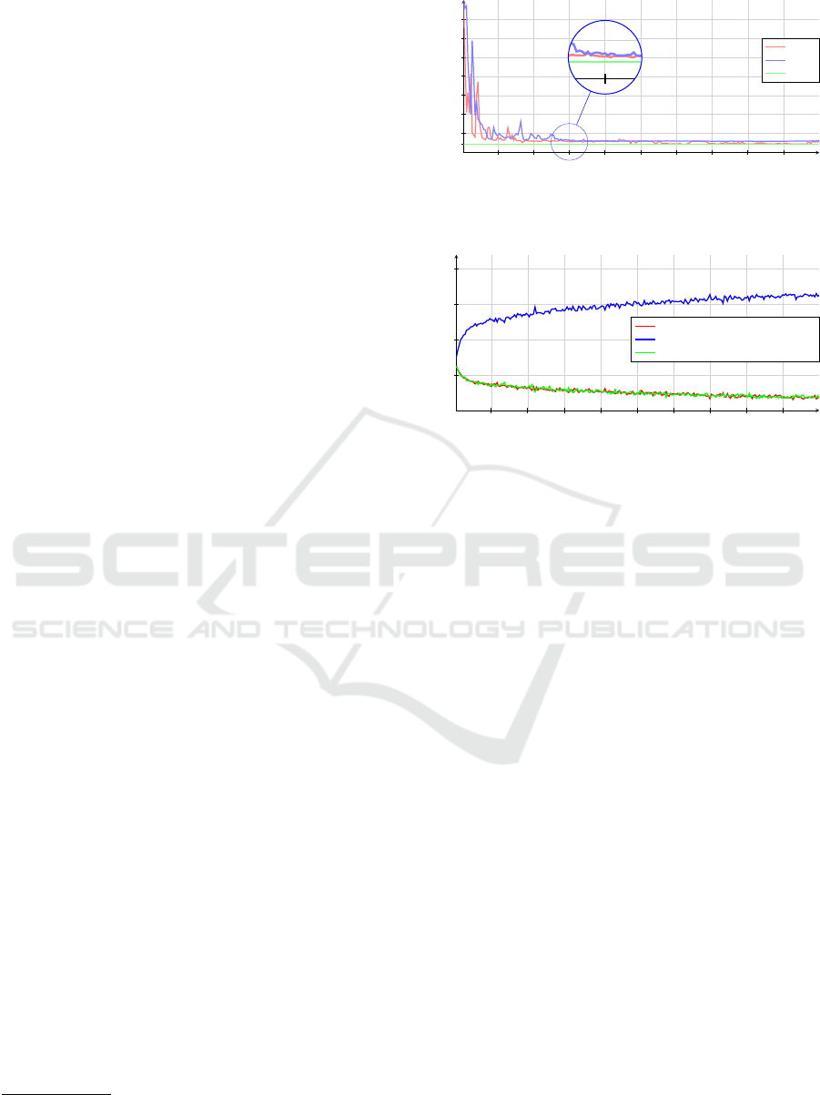
Figure 2: The number of steps, averaged over 10 episodes,

each approach requires to ﬁnish the episode, i.e., the car

reaching the top of the hill.

250 500 750 1000 1250 1500 1750 2000 2250

100

Episode number

Policy selection in the episode (average over 10 episodes)(%)

Time penalty policy

Backward acceleration penalty policy

Forward acceleration penalty policy

Figure 3: The percentage each policy in DWN agent selects

in an episode, averaged over 10 episodes.

The environment has three different objectives:

time penalty, backward acceleration penalty, and for-

ward acceleration penalty. As the name of each pol-

icy suggests, the time policy gives a negative re-

ward in every time step, except in the state when

the agent reaches the top, the backward acceleration

policy gives a negative reward when the agent is ac-

celerating backward, and analogously, forward accel-

eration penalty applies for the forward policy. The

agent has three available actions: accelerate forwards,

accelerate backward, or do nothing. We design the

DWN agent with three policies, one for each objec-

tive. For simplicity, we use the same ANN struc-

ture for all policies and for both Q and W networks,

i.e., θ

,θ

∀i. We use a feedforward ANN

structure with two hidden layers, each with 128 neu-

rons. On the output layer, to ensure better stability

of learning, we employ a dueling network architec-

ture (Wang et al., 2016), with 256 neurons. We list

hyper-parameters in Table 1.

In Fig. 2 we show the average number of steps, av-

eraged over ten episodes, the agent requires to reach

the top of the hill. The proposed DWN and DQN

algorithms both achieve similar performance in the

same number of episodes. Note that the DQN re-

ceives the reward in the form of a sum of three re-

ward signals, one for each policy the environment has.

Furthermore, for a fair comparison DQN employ the

same ANN structure as our DWN. Overall, the DWN

ICAART 2023 - 15th International Conference on Agents and Artiﬁcial Intelligence

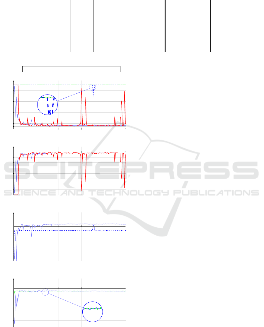
Table 1: Hyperparameters for the Mountain Car Environment.

Hyperparameter Value Hyperparameter Value Hyperparameter Value

γ 0.99 α

1 ∗ 10

−3

β 0.4

start

0.95

decay

0.995

min

0.1

start

0.99

decay

0.9995

min

0.1

ζ 0.6

1 ∗ 10

−3

1 ∗ 10

−3

Batch size K 1024 Memory size M

1 ∗ 10

Q Optimizer Adam

W Optimizer Adam Q learning rate

1 ∗ 10

−3

W learning rate

1 ∗ 10

−3

500 1000 1500 2000

110

250

500

750

1,000

1,250

1,500

1,750

2,000

Episode number

Average number of steps (over 10 episodes)

(a) Number of steps to reach the top

DWN

Time Policy Backward Policy Forward Policy

500 1000 1500 2000

−250

−500

−750

−1,000

−1,250

−1,500

−1,750

−2,000

Episode number

Average collected reward (over 10 episodes)

(b) Time Policy Performance

500 1000 1500 2000

−250

−500

Episode number

Average collected reward (over 10 episodes)

500 1000 1500 2000

−250

−500

−750

Episode number

Average collected reward (over 10 episodes)

(d) Forward Acceleration Performance

500 1000 1500 2000

110

250

500

750

1,000

1,250

1,500

1,750

2,000

Episode number

Average number of steps (over 10 episodes)

(a) Number of steps to reach the top

DWN

Time Policy Backward Policy Forward Policy

500 1000 1500 2000

−250

−500

−750

−1,000

−1,250

−1,500

−1,750

−2,000

Episode number

Average collected reward (over 10 episodes)

(b) Time Policy Performance

500 1000 1500 2000

−250

−500

Episode number

Average collected reward (over 10 episodes)

500 1000 1500 2000

−250

−500

−750

Episode number

Average collected reward (over 10 episodes)

(d) Forward Acceleration Performance

500 1000 1500 2000

110

250

500

750

1,000

1,250

1,500

1,750

2,000

Episode number

Average number of steps (over 10 episodes)

(a) Number of steps to reach the top

DWN

Time Policy Backward Policy Forward Policy

500 1000 1500 2000

−250

−500

−750

−1,000

−1,250

−1,500

−1,750

−2,000

Episode number

Average collected reward (over 10 episodes)

(b) Time Policy Performance

500 1000 1500 2000

−250

−500

Episode number

Average collected reward (over 10 episodes)

500 1000 1500 2000

−250

−500

−750

Episode number

Average collected reward (over 10 episodes)

(d) Forward Acceleration Performance

Figure 4: The comparison of performance between a pol-

icy as standalone DQN agent and a policy as a part of the

proposed DWN.

performance is similar, albeit slightly more stable, to

DQN in the mountain car environment. A far more in-

teresting analysis is in individual policy performance

by itself or part of DWN.

In Fig. 3 we show the percentage, i.e., how many

times the DWN agent has selected an individual pol-

icy in an episode. At the start, the agent selects poli-

cies evenly. Such a behaviour is expected due to high

starting epsilon-greedy value. However, as the epsilon

decays with the number of episodes and Q-learning

DQN learn, the agent starts to prefer one policy over

the others. Interestingly, the backward accelerating

policy proves to prevailing policy as the DWN selects

it three times more often the other two policies com-

bined.

In Fig. 4 we compare DWN with the performance

of DQN when it receives only the reward of a particu-

lar policy. In Fig. 4 (a), we show the number of steps

each policy requires to reach the top. Besides DWN

and the DQN with time policy will reach the objec-

tive, i.e., arrive at the top of the hill. It appears, that

when the reward signal is the only backward and for-

ward policy the agent is unable, with a small excep-

tion, to learn to reach the top. However, when we look

at the amount of collected reward a particular policy

collects as part of DWN or individually is almost the

same. Meaning, that without exception policies learn

to maximise their rewards. Note that the difference of

100 in Fig. 4 (c) between DWN and backward accel-

eration policy is due to the reward signal. The agent

receives a reward of 100 when it reaches the top, and

the backward policy reaches the top only as part of

DWN not individually.

Combining the gained insights from the above

results, we demonstrate that DWN performs as ex-

pected: the agent is capable of reaching the end objec-

tive, while also maximise the reward collected by the

individual policies within the DWN agent. In other

words, policies in DWN are selected in such a way

that on an individual level each policy can achieve

its best performance, i.e., maximise its long-term re-

wards. An added beneﬁt is that the agent can also

reach the main objective, i.e., reach the top of the hill.

Deep W-Networks: Solving Multi-Objective Optimisation Problems with Deep Reinforcement Learning

1000 2000 3000 4000 5000

−20

−10

Episode number

Averaged over 50 episodes

(a) Time penalty collected

DWN

DQN Time DQN Treasure DQN

1000 2000 3000 4000 5000

Episode number

Average over 50 episodes

(b) Treasure Collected

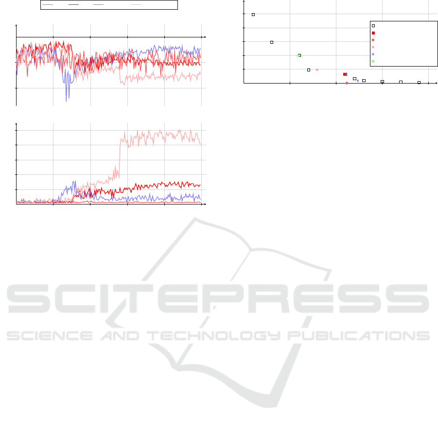
Figure 5: Time penalty and treasure collected, averaged

over 50 episodes, for the number of episodes.

4.2 Deep Sea Treasure

The second environment, called Deep Sea Treasure,

is a simple grid-world with treasure chests that in-

crease in value the deeper they are. The deeper the

chest is, the further away from the agent it is. The

goal of this scenario is for the agent to learn to opti-

mise for future rewards rather than opting for the frac-

tional short-term gain. We used the environment as

proposed and implemented in (Vamplew et al., 2011).

The deep sea environment has two objectives:

time penalty and collected treasure. The time objec-

tive is for the agent to ﬁnish the episode, i.e., ﬁnd the

treasure, as quickly as possible. Therefore, the agent

receives a negative reward of -1 at every step. The

treasure reward depends on how deep is the treasure.

Furthermore, the reward is increasing non-linearly

with the depth and ranges from 1 to 124. In this sce-

nario, our DWN agent has two policies: time and trea-

sure. As in the previous environment, all ANN, i.e.,

,θ

∀i, have the same Convolutional Neu-

ral Network (CNN) structure. The ﬁrst 2-dimensional

convolution layer has three input channels and 16 out-

put channels, and the second and third convolution

layers have 32 channels. Every convolution layer has

kernel size ﬁve with stride two, followed by batch nor-

malisation. The last dense layer in the ANN has 1568

neurons. We list hyper-parameters in Table 2.

First, we analyse the performance of individual

policies and compare it with DWN. For the individ-

ual policy, we employed DQN with the same neural

-15 -10 -5 0

100

125

Time cost

Treasure value

Pareto front

DQN

Time DQN

Treasure DQN

DWN without Pre-training

DWN with Pre-training

Figure 6: The Pareto front for the deep sea treasure environ-

ment.

structure as described above. In Fig. 5 we show the

performance of three DQN solutions, each with dif-

ferent reward signal. The ﬁrst DQN solution receives

only the time penalty reward signal, the second only

the treasure value signal, and the third the sum of the

two reward signals. The DQN with only time reward

learns to ﬁnish the episodes as fast as possible. There-

fore, it learns to collect the ﬁrst available treasure.

The DQN with only treasure reward learns to collect

the highest treasure reward of all approaches. How-

ever, it does not learn to collect the highest treasure

rewards, i.e., 74 and 124. The performance of DQN

with the sum of two rewards is exactly in the middle

of the two. Interestingly, the DWN performance is be-

tween the DQN with the sum reward and DQN with

only time reward.

In Fig. 6 we show how close to the Pareto front

the agent with a different approach can arrive after

5000 episodes. Note that results are the average of

the last one hundred episodes. The DQN learns to

reach the Pareto front. However, the collected trea-

sure reward is far from ideal. The DWN, when trained

from scratch, is close but under-performs in compari-

son to a DQN approach. Interestingly, DWN with pre-

trained Q-networks ﬁnds a high treasure at the Pareto

front. In the latter approach, we took advantage of

DWN modularity properties. First, we trained time

and treasure policy for 2500 episodes separately, and

then for 2500 episodes, we trained as part of DWN.

Such a behaviour can be explained that policies as part

of DWN are not able to converge, thus giving them a

head start, i.e., learning separately, can improve the

DWN performance. Furthermore, such a result was

expected because, as it was pointed out in the origi-

nal W-learning paper, we need to allow the Q-learning

networks to learn ﬁrst.

5 CONCLUSION

In this paper, we have proposed a deep learning ex-

tension to W-learning, an approach that naturally re-

ICAART 2023 - 15th International Conference on Agents and Artiﬁcial Intelligence

Table 2: Hyperparameters for the Deep Sea Environment.

Hyperparameter Value Hyperparameter Value Hyperparameter Value

γ 0.9 α

1 ∗ 10

−3

β 0.4

start

0.95

decay

0.995

min

0.25

start

0.99

decay

0.9995

min

0.01

ζ 0.6

1 ∗ 10

−3

1 ∗ 10

−3

Batch size K 1024 Memory size M

1 ∗ 10

Q Optimizer RMSprop

W Optimizer RMSprop Q learning rate

1 ∗ 10

−3

W learning rate

1 ∗ 10

−3

solves competition in multi-objective scenarios. We

have demonstrated the proposed method’s efﬁciency

and superiority to a baseline solution in two environ-

ments: deep sea treasure and multi-objective moun-

tain car. In both of these environments, the proposed

DWN is capable of ﬁnding the Pareto front. Fur-

thermore, we have also demonstrated the advantage

of DWN modularity properties by showing that us-

ing a pre-trained policy can aid in ﬁnding the Pareto

front in the deep sea treasure environment. In our fu-

ture work, we will focus on improving the compu-

tational performance and evaluating the performance

in more complex environments, e.g., SuperMario-

Bros (Kauten, 2018).

The proposed DWN algorithm can be employed

in any system with multiple objectives such as traf-

ﬁc control, telecommunication networks, ﬁnance, etc.

The condition being that each objective is represented

with a different reward function. The main advantage

of DWN is its ability to train multiple policies simul-

taneously. Furthermore, sharing the state space be-

tween policies is not mandatory, e.g., a policy for the

mountain car environment policies could only need

access to the velocity vector. Meaning that with DWN

it is possible to train policies with different states due

to the use of separate buffers for storing experiences.

ACKNOWLEDGEMENTS

This work was funded in part by the SFI-NSFC Part-

nership Programme Grant Number 17/NSFC/5224

and SFI under Frontiers for the Future project

21/FFP-A/8957.

REFERENCES

Abels, A., Roijers, D., Lenaerts, T., Now

e, A., and Steck-

elmacher, D. (2019). Dynamic weights in multi-

objective deep reinforcement learning. In Interna-

tional Conference on Machine Learning, pages 11–20.

PMLR.

Cardozo, N. and Dusparic, I. (2020). Learning run-time

compositions of interacting adaptations. SEAMS ’20,

page 108–114, New York, NY, USA. Association for

Computing Machinery.

Dusparic, I., Taylor, A., Marinescu, A., Cahill, V., and

Clarke, S. (2015). Maximizing renewable energy use

with decentralized residential demand response. In

2015 IEEE First International Smart Cities Confer-

ence (ISC2), pages 1–6.

Giupponi, L., Agusti, R., P

erez-Romero, J., and Sallent,

O. (2005). A novel joint radio resource manage-

ment approach with reinforcement learning mecha-

nisms. In IEEE International Performance, Comput-

ing, and Communications Conference (IPCCC), pages

621–626. Phoenix, AZ, USA.

Hribar, J., Marinescu, A., Chiumento, A., and DaSilva,

L. A. (2022). Energy Aware Deep Reinforce-

ment Learning Scheduling for Sensors Correlated in

Time and Space. IEEE Internet of Things Journal,

9(9):6732–6744.

Humphrys, M. (1995). W-learning: Competition among

selﬁsh Q-learners.

Jin, Y. and Sendhoff, B. (2008). Pareto-Based Multiobjec-

tive Machine Learning: An Overview and Case Stud-

ies. IEEE Transactions on Systems, Man, and Cyber-

netics, Part C (Applications and Reviews), 38(3):397–

415.

Karlsson, J. (1997). Learning to solve multiple goals. Uni-

versity of Rochester.

Kauten, C. (2018). Super Mario Bros for OpenAI Gym.

GitHub: github.com/Kautenja/gym-super-mario-bros.

Kusic, K., Ivanjko, E., Vrbanic, F., Greguric, M., and Dus-

paric, I. (2021). Spatial-temporal trafﬁc ﬂow control

on motorways using distributed multi-agent reinforce-

ment learning. Mathematics - Special Issue Advances

in Artiﬁcial Intelligence: Models, Optimization, and

Machine Learning, 9(23).

LeCun, Y., Bengio, Y., and Hinton, G. (2015). Deep learn-

ing. nature, 521(7553):436–444.

Liu, C., Xu, X., and Hu, D. (2015). Multiobjective Re-

inforcement Learning: A Comprehensive Overview.

IEEE Transactions on Systems, Man, and Cybernet-

ics: Systems, 45(3):385–398.

Mnih, V., Kavukcuoglu, K., Silver, D., Graves, A.,

Antonoglou, I., Wierstra, D., and Riedmiller, M.

(2013). Playing Atari With Deep Reinforcement

Learning. arXiv preprint arXiv:1312.5602.

Deep W-Networks: Solving Multi-Objective Optimisation Problems with Deep Reinforcement Learning

Mossalam, H., Assael, Y. M., Roijers, D. M., and White-

son, S. (2016). Multi-Objective Deep Reinforcement

Learning. arXiv preprint arXiv:1610.02707.

Nguyen, T. T., Nguyen, N. D., Vamplew, P., Nahavandi, S.,

Dazeley, R., and Lim, C. P. (2020). A multi-objective

deep reinforcement learning framework. Engineering

Applications of Artiﬁcial Intelligence, 96:103915.

Schaul, T., Quan, J., Antonoglou, I., and Silver, D.

(2015). Prioritized experience replay. Presented

at International Conference on Learning Representa-

tions (ICLR), San Diego, CA, May 7–9, 2015. arXiv

preprint 1511.05952.

Sprague, N. and Ballard, D. (2003). Multiple-goal rein-

forcement learning with modular sarsa(0). In 18th Int.

Joint Conf. Artif. Intell., page 1445–1447.

Tajmajer, T. (2018). Modular multi-objective deep rein-

forcement learning with decision values. In 2018 Fed-

erated conference on computer science and informa-

tion systems (FedCSIS), pages 85–93. IEEE.

Vamplew, P., Dazeley, R., Berry, A., Issabekov, R., and

Dekker, E. (2011). Empirical evaluation methods

for multiobjective reinforcement learning algorithms.

Machine learning, 84(1):51–80.

Wan, R., Zhang, X., and Song, R. (2020). Multi-objective

reinforcement learning for infectious disease control

with application to COVID-19 spread. arXiv preprint

arXiv:2009.04607.

Wang, Z., Schaul, T., Hessel, M., Hasselt, H., Lanctot, M.,

and Freitas, N. (2016). Dueling network architectures

for deep reinforcement learning. In Proceedings of

Machine Learning Research (PMLR), vol.48, pages

1995–2003. New York, USA.

ICAART 2023 - 15th International Conference on Agents and Artiﬁcial Intelligence