Visualizing Grassmannians via Poincare Embeddings

Huanran Li

and Daniel Pimentel-Alarcón

Department of Electrical Engineering, Wisconsin Institute for Discovery University of Wisconsin-Madison, U.S.A.

Department of Biostatistics, Wisconsin Institute for Discovery University of Wisconsin-Madison, U.S.A.

Keywords:

Grassmannian, Manifold Learning, Poincare Disk, t-SNE, High-Dimensional Data and Dimensionality

Reduction.

Abstract:

This paper introduces an embedding to visualize high-dimensional Grassmannians on the Poincaré disk,

obtained by minimizing the KL-divergence of the geodesics on each manifold. Our main theoretical result

bounds the loss of our embedding by a log-factor of the number of subspaces, and a term that depends on the

distribution of the subspaces in the Grassmannian. This term will be smaller if the subspaces form well-deﬁned

clusters, and larger if the subspaces have no structure whatsoever. We complement our theory with synthetic and

real data experiments showing that our embedding can provide a more accurate visualization of Grassmannians

than existing representations.

1 INTRODUCTION

Subspaces are a cornerstone of data analysis, with ap-

plications ranging from linear regression to principal

component analysis (PCA) Knudsen (2001); Jansson

and Wahlberg (1996); Vaswani et al. (2018), low-rank

matrix completion (LRMC) Dai et al. (2011); Vidal

and Favaro (2014), computer vision Cao et al. (2016);

Chen and Lerman (2009); Hong et al. (2006); Lu and

Vidal (2006), recommender systems Koohi and Kiani

(2017); Ullah et al. (2014); Zhang et al. (2021), classiﬁ-

cation Sun et al. (2015); Ahmed and Khan (2009); Xia

et al. (2017), and more Van Overschee (1997); Mevel

et al. (1999). However, there exist few tools to visual-

ize the Grassmann manifold

G(m,r)

-dimensional

subspaces of

. Perhaps the most intuitive of such

visualizations is the representation of

G(3,1)

as the

closed half-sphere where each point in the hemisphere

represents the 1-dimensional subspace (line) in

that

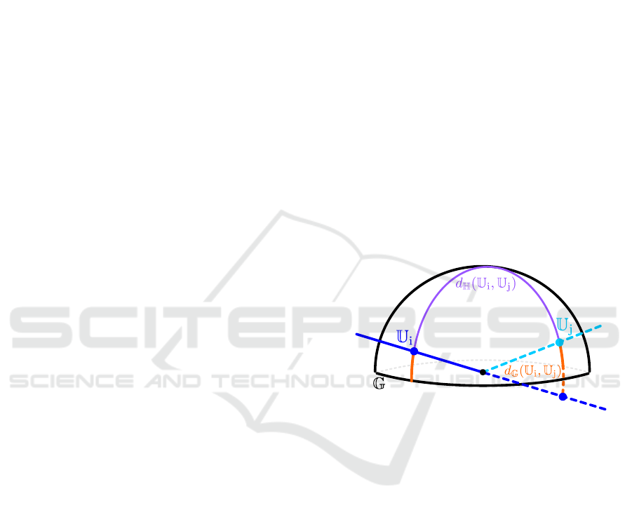
crosses that point and the origin (see Figure 1). While

intuitive, this visualization bears certain limitations.

First, this representation wraps around the edge, so

geodesic distances can be deceiving. For instance, two

points (subspaces) that may appear diametrically far

may in fact be arbitrarily close (see Figure 1). But

more importantly, the main caveat of this semi-sphere

representation is that it is unclear how to generalize it

m > 3

r > 1

, which makes it quite restrictive, spe-

cially for analysis of modern high-dimensional data.

Motivated by this gap, we propose visualizing a

collection of points in the Grassmannian (subspaces)

Figure 1: Classical 3D Representation of the Grassmannian

G(3,1)

. Each point represents the subspace

that connects

that point to the origin. This representation wraps around the

edge. Two points (subspaces) that appear diametrically far

w.r.t. the geodesic distance on the hemisphere (

)

are in fact close w.r.t. the geodesic distance on the Grassman-

nian (

)

; see

(1)

). An intuitive way to see this is to

extend the lines to the opposite side of the hemisphere and

compute their smallest angle.

through an embedding onto the Poincaré disk

D ⊂ R

This embedding, which we call GrassCaré, is inspired

by the well-known t-Distributed Stochastic Neighbor

Embedding (t-SNE), which is widely used to visualize

high-dimensional data (in

) on the

plane while

preserving Euclidean distances in

Van der Maaten

and Hinton (2008). The main difference between the

t-SNE and our GrassCaré embedding is that the latter

maps points in

G(m,r)

onto

while preserving the

geodesics on the Grassmannian as much as possible.

This allows to keep an accurate global representation

of the Grassmannian in a unit circle while at the same

time retaining any local structures. Our embedding

Li, H. and Pimentel-Alarcón, D.

Visualizing Grassmannians via Poincare Embeddings.

DOI: 10.5220/0011609400003417

In Proceedings of the 18th International Joint Conference on Computer Vision, Imaging and Computer Graphics Theory and Applications (VISIGRAPP 2023) - Volume 3: IVAPP, pages 27-39

ISBN: 978-989-758-634-7; ISSN: 2184-4321

 2023 by SCITEPRESS – Science and Technology Publications, Lda. Under CC license (CC BY-NC-ND 4.0)

is obtained by minimizing the Kullback-Leibler (KL)

divergence between the geodesics on the Grassman-

nian and the Poincaré disk using Riemannian gradient

descent. Our main theoretical result shows that the

loss of our embedding (measured in terms of the KL-

divergence with respect to (w.r.t.) the Grassmannian

geodesics) is bounded by a log-factor of the number of

subspaces, and a term that depends on the distribution

of the subspaces in the Grassmannian. This term will

be smaller if the subspaces form well-deﬁned clusters,

and it will be larger if the subspaces have no structure

whatsoever. In words, this result shows that under

reasonable assumptions, our embedding can be an ac-

curate representation of the Grassmannian. Equipped

with this result, we believe that the GrassCaré em-

bedding can be a powerful tool for subspace tracking,

classiﬁcation, multi-dataset analysis, and any applica-

tion where there is an interest in visualizing subspaces.

This paper should be understood as a ﬁrst introduction

of our embbedding method, a development of funda-

mental theory, and an exploration of its performance

on canonical datasets.

Paper Organization. In Section 2 we discuss several

applications of our GrassCaré embedding. Section

3 brieﬂy summarizes related work. In Section 4 we

introduce the main formulation that determines our

embedding, together with the gradient steps for the

optimization. Section 5 presents our main theorem,

bounding the loss of our embedding, followed by its

proof. Finally, in Section 6 and 7 we demonstrate the

applicability of our GrassCaré embedding on real and

synthetic data, we compare it to naive alternatives, and

we discuss its advantages and limitations.

2 APPLICATIONS

Our GrassCaré embedding could be a valuable tool in

the following applications:

Subspace Clustering: aims to cluster a collection of

data points

x ∈ R

lying near a union of subspaces

Parsons et al. (2004). Equivalently, the goal is to

ﬁnd a union of subspaces that approximates a high-

dimensional dataset. This method has applications in

motion segmentation Yang et al. (2008); Vidal et al.

(2008), face clustering Elhamifar and Vidal (2013),

data mining Agrawal et al. (1998), time series Ba-

hadori et al. (2015), and more. As we show in our

experiments, our GrassCaré embedding can aid ana-

lyzing the results of a subspace clustering algorithm

beyond a simple accuracy metric, providing insights

and summaries about the clusters characteristics and

relationships. It can also be a valuable tool for debug-

ging and understanding algorithmic performance. In

fact, analyzing and understanding a subspace cluster-

ing algorithm is what initially motivated this paper.

Low-Rank Matrix Completion: aims to recover the

missing entries of a low-rank matrix

Recht (2011).

This is equivalent to ﬁnding the low-dimensional row

and column spaces of

. Some applications of LRMC

include recommender systems Kang et al. (2016), im-

age processing Ji et al. (2010), drug discovery Zhang

et al. (2019), and electronic health records (EHR) Lee

et al. (2010). As we show in our experiments, our

GrassCaré embedding can help analyze the algorith-

mic behavior of LRMC methods as they make opti-

mization steps to complete

, showing proximity to

the target, convergence, step sizes, and patterns as they

move through the Grassmannian.

Subspace Tracking: aims to constantly estimate a

subspace

that changes over time (moves in the

Grassmannian), based on iterative observations

∈U

Vaswani et al. (2018); He et al. (2011); Xu et al. (2013).

This model has applications in signal processing Stew-

art (1998), low-rank matrix completion Balzano et al.

(2010), and computer vision He et al. (2011), where,

for example, one may want to estimate the subspace

corresponding to the moving background of a video.

Here our GrassCaré embedding can be used to track

the subspace path as it moves through the Grassman-

nian. This could provide insights about the subspaces’

behavior: moving speed and distance, zig-zag or cy-

cling patterns, etc.

Multi-Dataset Analysis. Principal Component Analy-

sis (PCA) is arguably the most widely used dimension-

ality reduction technique, with applications ranging

from EHR Lee et al. (2010) to genomics Novembre

et al. (2008); Song et al. (2019) to vehicle detection

Wu and Zhang (2001); Wu et al. (2001). In a nutshell,

PCA identiﬁes the low-dimensional subspace that best

approximates a high-dimensional dataset. In modern

situations, several of these datasets may be distributed

or related in some way. For instance, the EHRs of

a population of certain location could be tightly re-

lated to those of another. However, due to privacy

concerns, security, size, proprietorship, and logistics,

exchange of information like this could prove chal-

lenging if not impossible. The principal subspaces,

however, could be efﬁciently shared without many of

these concerns, potentially providing new informative

insights. Our GrassCaré embedding could provide a

visualization tool to analyze the relationships between

related datasets like these, potentially revealing simi-

larities, clusters and patterns.

IVAPP 2023 - 14th International Conference on Information Visualization Theory and Applications

3 PRIOR WORK

To the best of our knowledge, general visualiza-

tions of Grassmannians have been studied using Self-

Organizing Mappings (SOM) Kirby and Peterson

(2017), which were introduced ﬁrst for general dimen-

sionality reduction Kohonen (1982, 1990, 1998, 2013).

The extension of SOM to Grassmannians iteratively

updates points on a 2D index space to ﬁnd the best

arrangement, such that points that are neighbors in the

Grassmannian are still close in the embedding. How-

ever, SOM present several limitations. For instance,

like most neural networks, they require large datasets,

which may not always be available in practice. They

also suffer of large parameter spaces, and are quite

difﬁcult to analyze, making it hard to derive theoreti-

cal guarantees about the accuracy of their embeddings.

It is worth mentioning that there are numerous meth-

ods for general high-dimensional data visualization,

including umapMcInnes et al. (2018), LargeVisTang

et al. (2016), Laplacian eigenmaps Belkin and Niyogi

(2001, 2003), isomap Tenenbaum et al. (2000), and

more Liu et al. (2016); Engel et al. (2012); Ashokku-

mar and Don (2017); Kiefer et al. (2021). However,

since these embeddings are not compact, they are not

appropriate to represent the Grassmannian.

Another more suitable alternative are the Grass-

mannian Diffusion Maps (GDMaps) dos Santos et al.

(2020) introduced as an extension of Diffusion Maps

Coifman et al. (2005). GDMaps consist of two seper-

ate stages. The ﬁrst stage projects the given data point

(i.e. vector, matrix, tensor) onto the Grassmannian us-

ing a singular value decomposition. The second stage

uses diffusion maps to identify the subspace structures

on the projected Grassmannian. Although the embed-

ding can be quickly generated, it is unfortunately less

accurate than other methods in this paper. On the other

hand, Stochastic Neighbor Embeddings (SNE) were

ﬁrst presented by Hinton and Roweis in Hinton and

Roweis (2002). It formed the basis for t-SNE, which

was introduced later by Maaten and Hinton in Van der

Maaten and Hinton (2008). Both algorithms minimize

the KL-divergence between the distributions represent-

ing the probability of choosing the nearest neighbor on

the high and low dimensional spaces. These embed-

dings have become some of the most practical tools

to visualize high dimensional data on Euclidean space.

However, Euclidean distances are poor estimators of

geodesics of Grassmannians, so a direct application of

these methods would result in an inaccurate represen-

tation of subspaces arrangements.

Motivated by these issues we decided to explore the

use of the Poincaré disk, which has recently received

increasing attention for high-dimensional embeddings

Nickel and Kiela (2017); Klimovskaia et al. (2020).

Intuitively, the Poincaré disk is a 2D hyperbolic geo-

metric model, usually displayed as a unit circle where

the geodesic distance between two points in the disk

is represented as the circular arc orthogonal to the unit

circle Goodman-Strauss (2001), which corresponds to

the projection of the hyperbolic arc of their geodesic

(see Figure 2 to build some intuition). This unique

feature brings several advantages for serving as the

embedding space for Grassmannian. First, since these

hyperbolic arcs get larger (tending to inﬁnity) as points

approach the disk boundary, the Poincaré disk is an

effective model to accurately represent the global struc-

ture of complex hierarchical data while retaining its

local structures. Speciﬁcally, the Poincaré disk can

be viewed as a continuous embedding of tree nodes

from the top of the tree structure, where the root node

is at the origin, and the leaves are distributed near

the boundary. So, it is naturally suited to represent

hierarchical structures. This is suitable to represent

structured clusters, where the points from the same

cluster can be regarded a branch of the tree, because

they share a similar distance to other clusters. Sec-

ond, the hyperbolic disk has a Riemannian manifold

structure that allow us to perform gradient-based opti-

mization, which is crucial to derive convergence guar-

antees, and for parallel training of large-scale dataset

models. Finally, our main result showing the accuracy

of our embedding enables efﬁcient clustering using the

Poincaré low-dimensional representation. That is, in-

stead of clustering subspaces on the high-dimensional

dataset, the clustering method can be performed on the

mutual distances acquired from the embedding, with

the knowledge that the embedding would represent the

high-dimensional subspace accurately enough.

4 SETUP AND FORMULATION

In this section we present the mathematical formula-

tion of our GrassCaré embedding. To this end let us

ﬁrst introduce some terminology. Recall that we use

G(m,r)

to denote the Grassmann manifold that con-

tains all the

-dimensional subspaces of

. For any

two subspaces

∈G(m,r)

, the geodesic distance

between them is deﬁned as:

) :=

∑

ℓ=1

arccos

ℓ

), (1)

where

∈ R

m×r

are orthonormal bases of

and

ℓ

(·)

denotes the

ℓ

largest singular value. As for

the embedding space, recall that the Poincaré disk

the Riemannian manifold deﬁned as the open unit ball

Visualizing Grassmannians via Poincare Embeddings

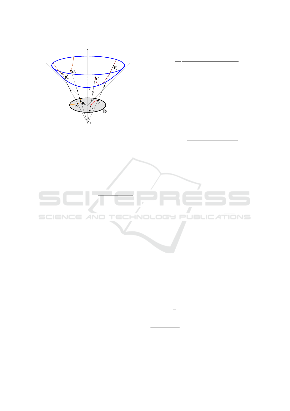
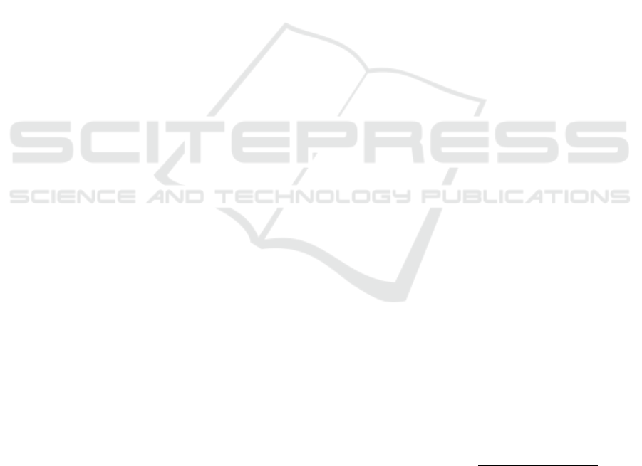
Figure 2: Geodesics in the Poincaré disk

. The geodesic

distance

)

is given by the Euclidean length of the

hyperbolic arc between

′

and

′

, and is often depicted in

the disk by the arc between

and

(and similarly for

)

). Points closer to the disk’s boundary will be

projected higher on the hyperbolic space, resulting in larger

distances (see

(2)

). In words, distances near the edge are

larger than they appear.

equipped with the following distance function

between two points p

∈ D:

) := arcosh



1 + 2

∥p

−p

∥

(1−∥p

∥

)(1−∥p

∥

)



(2)

Notice from

(2)

that the geodesic distance in the disk

is ampliﬁed smoothly as

move away from

the origin. Intuitively, this means that an arc of the

same Euclidean length in the disk represents a larger

geodesic distance (tending to inﬁnity) as it approaches

the edge of the disk. In other words, distances near the

edge of the disk are larger than they appear (see Figure

3 to build some intuition). Conversely, distances at

the center of the disk are smaller than they appear.

This allows to plot denser regions of the Grassmannian

with higher granularity (thus retaining local structure)

while at the same time keeping an accurate global

representation of the Grassmannian inside an open

circle.

To ﬁnd our embedding, we will mimic the sym-

metric SNE approach in Van der Maaten and Hinton

(2008). That is, we will ﬁrst compute a probability

matrix

∈ [0,1]

N×N

whose

(i,j)

entry represents

the probability that

is chosen as a nearest neighbor

, which is equal to zero if

i = j

, and for

i ̸= j

given by:

]

exp(−d

)

/2γ

)

∑

k̸=i

exp(−d

)

/2γ

)

exp(−d

)

/2γ

)

∑

k̸=j

exp(−d

)

/2γ

)

, (3)

where

is adapted to the data density: smaller values

for denser regions of the data space. In our experi-

ments, we choose it to be the variance of distances

from point

to other points. Next we create the proba-

bility matrix

∈ [0, 1]

N×N

, whose

(i,j)

entry repre-

sents the probability that point

in our embedding

is chosen as a nearest neighbor of point

∈ D

, which

is equal to zero if i = j, and for i ̸= j is given by:

]

exp(−d

)

/β)

∑

k̸=l

exp(−d

)

/β)

(4)

where

β > 0

(usually set to

) controls the em-

bedding’s scattering Klimovskaia et al. (2020). The

larger

, the smaller variance in the probability matrix

. In practice, we did not notice much variability

in our results as a function of this parameter. Thus,

following standard practice Klimovskaia et al. (2020),

we pick

β = 1

. Our goal to obtain the embedding is

to maximize the similarity between the two distribu-

tions

and

, which we do by minimizing their

Kullback-Leibler (KL) divergence:

KL(P

||P

) =

∑

i,j

]

log

]

Since

is a constant given

}

, this is the same as

minimizing the following loss

L = −

∑

i,j

]

log[P

]

To minimize this loss over the Poincaré disk

will use Riemannian Stochastic Gradient Descent

Bonnabel (2013), which updates p

t+1

according to:

t+1

← R(p

−η∇

L), (5)

where

η > 0

is the step size (set as

η = 1

in the im-

plementation),

∇

denotes the Riemannian gradient

w.r.t.

, and

denotes a retraction

from the

tangent space of p

onto D. It is easy to see that

∇

L =

∑

([P

]

−[P

]

)(1 + d

)

−1

·d

)∇

), (6)

A mapping

from the tangent bundle

T M

to the mani-

fold

such that its restriction to the tangent space of

satisﬁes a local rigidity condition which preserves gradi-

ents at

; see Chapters 3 and 4 of Absil et al. (2009) for a

more careful treatment of these deﬁnitions.

IVAPP 2023 - 14th International Conference on Information Visualization Theory and Applications

where the gradient of d

w.r.t. p

is given by:

∇

) =

√

−1

||p

−2⟨p

⟩+ 1

−

Here

a = 1 − ||p

b = 1 − ||p

, and

c = 1 +

||p

−p

. Finally, the retraction step is given by

R(p

−η∇

L) = proj



−η

(1 −||p

)

∇



where

proj(p

) =

(

/(||p

||+ ε) i f ||p

|| ≥ 1

otherwise,

and

is a small constant number; in our experiments

we set this to 10

−5

In our implementation we use random initialization

for the points in the embedding. We point out that ini-

tialization is crucial for t-SNE. This is because t-SNE

is generally used to embed points in the Euclidean

space, which is open. In contrast, the Grassmannian

is spherical and compact, and hence, we observed that

varying initialization resulted in similar/equivalent em-

beddings of the Grassmannian, observed from differ-

ent angles. This is further demonstrated in our exper-

iments section (Figure 5), where the average loss of

GrassCaré over 100 trials varies very little in compari-

son to all other embeddings, showing that besides this

point-of-view difference, our results do not depend

heavily on the initialization. The entire embedding

procedure is summarized in Algorithm 1.

Algorithm 1: GrassCaré.

Input: A collection of subspaces

,...,U

} ∈

G(m,r).

Output: A collection of points

,...,p

}

in the

Poincaré disk D.

Parameter: β ∈ [1,2],ε < 10

−5

Construct P

according to (3)

Randomly initialize p

,...,p

∈ D

repeat

Construct P

according to (4)

for i ∈ [1, N] do

Compute KL-loss gradient ∇

L as in (6)

Update point p

according to (5)

end for

until Converge

MAIN THEORETICAL RESULTS

AND PROOFS

First observe that convergence of our embedding fol-

lows directly by now-standard results in Riemannian

optimization (see e.g. Proposition in Adams et al.

(1996)). In fact, local convergence of our embedding

follows directly because our Riemannian steps are

gradient-related Adams et al. (1996). Our main theo-

retical result goes one step further, bounding the loss

of our embedding by a log-factor of the number of

subspaces, and a term that depends on the arrange-

ment of the subspaces in the Grassmannian. This term

will be smaller if the subspaces form well-deﬁned

clusters, and larger if the subspaces have no structure

whatsoever. Intuitively, this result shows that under

reasonable assumptions, our embedding can provide

an accurate representation of Grassmannians.

Theorem 1. Suppose

N > 3

. Deﬁne

γ := min

and

Γ := max

. Let

,...,U

}

be a partition

,...,U

}

such that

|≥n

> 1 ∀ k

. Let

δ :=

√

2γ

max

∈U

∆ :=

√

2Γ

min

∈U

ℓ

k̸=ℓ

Then the optimal loss of GrassCaré is bounded

by:

⋆

< log D +

−∆

β(n

−1)

where

D := N(n

−1) + N(N −n

)

·exp



−arcosh



1 +

2sin(π/K)

0.75



/β



. (7)

In words, Theorem 1 requires that the subspaces

can be arranged into clusters of size

> 1

such that

the intra-cluster distances are smaller than

√

2δγ

, and

the outer-cluster distances are larger than

√

2∆Γ

(see

Figure 3). Notice that this can always be done as long

N > 3

. However, depending on the arrangement,

could be too large or

∆

too small, resulting in a loose

bound. Ideally we want a small

and a large

∆

, so that

the subspaces form well-deﬁned clusters and

−∆

small, resulting in a tighter bound.

Proof.

Theorem 1 follows by a similar strategy as in

Shaham and Steinerberger (2017), which essentially

bounds the optimal loss by that of an artiﬁcial embed-

ding. In our case we will use an embedding that maps

,...,U

}

points uniformly distributed in the

circle of radius

1/2

, i.e.,

= p

for every

∈ U

(see Figure 3). This way, for any subspaces

Visualizing Grassmannians via Poincare Embeddings

Figure 3: Left: Theorem 1 requires that the intra-cluster dis-

tances are smaller than

√

2δγ

, and the outer-cluster distances

are larger than

√

2∆Γ

. Right: Example of the artiﬁcial em-

bedding (with

K = 5

) in the proof of Theorem 1, which maps

all subspaces in cluster

to the same point in the circle of

radius 1/2.

different clusters

ℓ

, the geodesic distance of their

embeddings on the Poincaré disk is upper and lower

bounded by

2.2 >



1 +

0.75



≥ d

)

≥ arcosh



1 +

2sin(π/K)

0.75



=: Φ.

It follows that the (i,j)

entry of P

is bounded by

]

exp(−d

)

/β)

∑

k̸=l

exp(−d

)

/β)

≥

exp(−d

)

/β)

N(n

−1) + N(N −n

)exp(−Φ

/β)

, (8)

where the denominator is precisely

as deﬁned in

(7)

Now, if

and

are in the same cluster

, the bound

(8)

simpliﬁes to

1/D

. Otherwise, it simpliﬁes to

exp(−2.2

/β)/D

. Plugging these bounds in the loss,

we see that:

∗

∑

i,j in same cluster

]

logD

∑

i,j in different clusters

]

(2.2

/β + log D)

≤ log D +

∑

i,j in different clusters

]

(2.2

/β). (9)

Next notice that if

are not in the same cluster,

]

exp(−d

)

/2γ

)

∑

k̸=i

exp(−d

)

/2γ

)

exp(−d

)

/2γ

)

∑

k̸=j

exp(−d

)

/2γ

)

≤

−∆

∑

k̸=i

exp(−d

)

/2γ

)

−∆

∑

k̸=j

exp(−d

)

/2γ

)

≤

−∆

N(n

−1)e

−δ

Plugging this into

(9)

we obtain the desired result.

6 EXPERIMENTS

Recall that the main motivation of this paper is to de-

velop a novel method to visualize Grassmannians of

high ambient dimension. Our bound above describes

the theoretical accuracy of our embedding. We now

present a series of experiments on real and synthetic

datasets to analyze its practical performance. In par-

ticular, we will test on normal simulated data, and

one canonical datasetTron and Vidal (2007). These

datasets have moderately high ambient dimension (i.e.,

many features), but low intrinsic dimension (i.e., lie

in a low-dimensional subspace). In other words, these

datasets would ﬁt in high-dimensional Grassmannians

of low-dimensional subspaces. We believe that these

well-studied datasets are a perfect ﬁt for our setting,

and convenient for an initial exploration and compari-

son against existing baselines.

Comparison Baseline. To evaluate the effectiveness

of our method we used t-SNEVan der Maaten and Hin-

ton (2008), GDMaps dos Santos et al. (2020), and a

naive visualization based on the most common dimen-

sionality reduction technique: Principal Components

Analysis (PCA). To this end we ﬁrst vectorize (stack

the columns of) each orthonormal basis

into a vec-

tor

∈ R

. Next we concatenate all vectors

into

a matrix of size

mr ×N

, on which we apply PCA. In

this naive PCA (nPCA) visualization, the subspace

is represented in the

(x,y)

plane by

∈ R

, the

coefﬁcients of u

w.r.t. the leading principal plane V.

Clustering Synthetic Data. In our synthetic experi-

ments we study our embedding when the subspaces are

uniformly distributed among

clusters. To this end we

ﬁrst generated

centers in the Grassmannian

G(m,r)

each deﬁned by a

m ×r

matrix

with i.i.e. standard

IVAPP 2023 - 14th International Conference on Information Visualization Theory and Applications

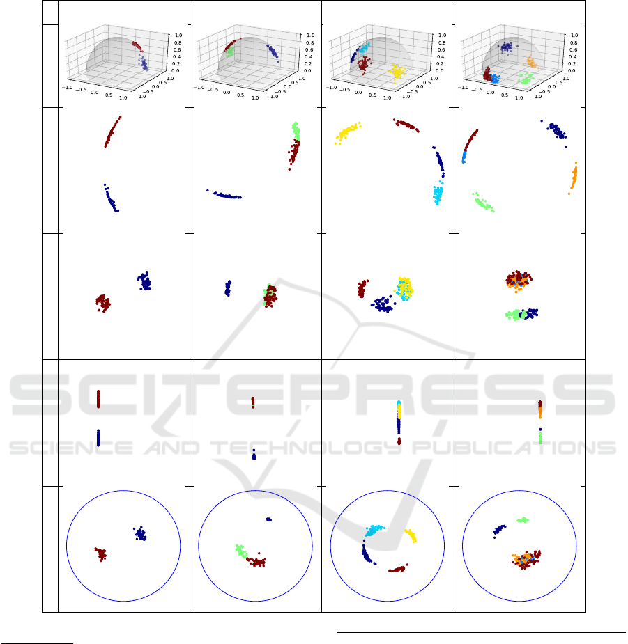
Classic 3D nPCA GDMaps t-SNE GrassCaré

Figure 4: Visualizations of clusters in

G(3,1)

with 4 clusters.

GrassCaré produces a more accurate

representation of the Grassmannian

. nPCA and even the 3D representation display Clusters 1 and 2 (cyan and yel-

low) nearly diametrically apart. In reality they are quite close, as depicted by GrassCaré.

normal entries whose columns are later orthonormal-

ized. Then for each

we independently generate

subspaces, each spanned by a basis

whose entries

are equal to those of

plus i.i.d. normal random vari-

ables with variance

. This will produce

clusters

G(m,r)

, each with

subspaces. The smaller

, the

closer the subspaces in the same cluster will be to one

another, and vice versa.

In our ﬁrst experiment we study a controlled setting

where we can actually visualize the low-dimensional

Grassmannian

G(3,1)

, and compare it with our em-

bedding on the Poincaré disk. We hope that this ex-

periment provides a visual intuition of how points are

embedded in higher-dimensional cases. To this end

we generated

= 50

subspaces per cluster (

m = 3

r = 1

), and we set

σ = 0.1

, which produced visually

well-deﬁned cluster clouds. Figure 4 shows some re-

sults for

K = 4

clusters (see Figure 9 in the Appendix

for additional values of

). At ﬁrst glance it might

appear like our GrassCaré embedding is not too dif-

ferent from the other approaches, especially as t-SNE

and nPCA seems to be doing a decent job displaying

the clusters. However, a more careful look reveals that

t-SNE clearly agglomerates several pairs of clusters,

while the GrassCaré can separate them nicely.

In particular, notice that in Figure 4, both nPCA

and even the classic 3D representation fail to show the

true local structure of the Grassmannian that the Grass-

Caré plot reveals. To see this pay special attention to

the cyan and yellow clusters. Based on the ﬁrst two

rows (classic 3D representation and nPCA) these clus-

ters would appear to be nearly diametrically apart (in

the 3D representation, the cyan cluster is in the back

side of the hemisphere). However, computing their

geodesics one can verify that the subspaces that they

represent are in fact quite close in the Grassmannian.

An intuitive way to see this is to extend the lines to

the opposite side of the hemisphere and compute their

smallest angle, or to remember that in the 3D repre-

sentation, the hemisphere wraps around the edge (see

Figure 3). In contrast, our GrassCaré plot accurately

displays the true global structure of the Grassman-

nian, mapping these two clusters close to one another.

Also notice that the embeddings are plotted with equal

scale on horizontal and vertical axis. The GrassCaré

makes a better use of the visual space, spreading all

data more broadly while at the same time keeping the

clusters well-deﬁned. In contrast, GDMaps has much

less range on the horizontal axis, which makes it look

like a straight line and not be able to display the full

information. More examples for different values of K

are presented in the Appendix.

The previous experiment shows the qualitative su-

periority of the GrassCaré embedding over alternative

embeddings in the low-dimensional case

m = 3

and

r = 1

(where no vectorization is needed for nPCA). In

our next experiment we will show in a more quanti-

tative way that the advantages of GrassCaré are even

more evident in higher dimensional cases. First notice

that the classic 3D representation only applies to the

case

m = 3

r = 1

, and there is no clear way how to

extend it to higher dimensions. On the other hand, re-

call that for

r > 1

, nPCA requires vectorizing the bases

, which will naturally interfere even more with the

structure of the Grassmannian. To see this consider:

U =





1 0

0 1

0 0





and U

′





0 1

1 0

0 0





While both span the same subspace in

G(3,2)

, the Eu-

clidean distance of their vectorizations is large, which

would result in distant points in the nPCA embed-

ding. t-SNE and GDMaps present similar inaccuracy

behavior. To verify this we generated subspaces in

the exact same way as described before (with

K = 3

= 17

, and different values of

and

), except this

time we measured the quality of the visualization in

terms of the representation error, which we deﬁne

as the Frobenius difference between the (normalized)

distance matrices produced by the subspaces in the

Grassmannian and the points in each embedding. In

the case of GrassCaré, distances in the embedding are

measured according to the Poincaré geodesics, so the

representation error of the GrassCaré embedding will

Visualizing Grassmannians via Poincare Embeddings

Figure 5: Representation error of GrassCaré (this paper) and other methods for high-dimensional Grassmannians G(m,r).

be measured as:

(D) =

∑

i,j



)

−

)



, (10)

where

∑

i,j

)

and

∑

i,j

)

are

normalization terms. Similarly, since the distance that

all other embeddings aim to minimize is Euclidean,

the representation error of the other embeddings will

be measured as:

(V) =

∑

i,j



)

−

∥v

−v

∥



, (11)

where

∑

i,j

∥v

−v

∥

is a normalization term.

The results of 100 trials are summarized in Figure 5,

which conﬁrms the superiority of our GrassCaré em-

bedding, and the loss of structure of the naive approach.

The computation time is also summarized in Figure 10

in the Appendix.

Subspace Estimation from Incomplete Data. In our

next experiment we apply our GrassCaré embedding

to visualize the path of subspaces produced by the

subspace estimation algorithm known as GROUSE

(Grassmannian Rank-One Update Subspace Estima-

tion) Balzano et al. (2010). The applicability of this

algorithm ranges from online video analysis (to track

the subspace of the background in real time) to sub-

space clustering Parsons et al. (2004) and low-rank

matrix completion (LRMC) Balzano et al. (2010). In

the latter, the algorithm receives a subset of the entries

of a data matrix

X ∈ R

m×n

whose columns lie in an

unknown subspace

⋆

∈ G(m, r)

, and the goal is to

estimate

⋆

. To this end GROUSE starts with a sub-

space estimate

∈ G(m, r)

, and iteratively tilts it in

the direction of a column of

, producing a sequence

of subspaces U

,...,U

To emulate this setup we ﬁrst generate true and

initial subspaces with bases

⋆

∈ R

m×r

with

i.i.d. standard normal entries. Next we generate

a coefﬁcient matrix

Θ ∈ R

r×n

with i.i.d. standard

normal entries, so that

X = U

⋆

is rank-

. Then

we run GROUSE using a fraction

Ω

of the en-

tries of

, selected uniformly at random. We store

each of GROUSE’s steps, and visualize their path

,...,U

(together with the target

⋆

) using our

GrassCaré embedding, nPCA, GDMaps, and t-SNE.

Figure 6 shows sample plots when

m = 200

r = 5

Ω = 0.7

(corresponding to 30% missing data; both

cases share the same initialization), and

n = N = 50

(corresponding to the case where GROUSE only it-

erates once over each column). Here once again

the GrassCaré plot shows a richer depiction of the

subspaces and a better usage of the available visual

space. From the GrassCaré plot we can clearly vi-

sualize each separate path, and see that, as expected,

the full-data estimate gets much closer to the target

than the missing-data estimate (and much faster). In

contrast, the paths in the nPCA plot are hardly dis-

tinguishable and misleading, showing the opposite of

the truth: an incomplete-data estimate much closer to

the target than the full-data estimate. To verify once

again (beyond our visual interpretation) that the Grass-

Caré embedding is much more representative of the

true distribution of subspaces in the Grassmannian, we

measured the distance of each iterate to the target, in

the Grassmannian and in each embedding. The nor-

malized results are in ﬁgure 7. They show that the

trajectories in the GrassCaré embedding mimic closely

those in the Grassmannian. In contrast, the nPCA em-

bedding can be quite misleading, showing in fact an

opposite representation, with distances in the embed-

ding growing over iterations, while in reality they are

decreasing in the Grassmannian.

Motion Segmentation. In our ﬁnal experiment we

use our GrassCaré plot to visualize the subspaces

describing moving objects in videos from the Hopkins

155 dataset Tron and Vidal (2007). This dataset

contains the locations over time of landmarks

of several moving objects (e.g., cars, buses, or

checkerboards) in 155 video sequences. Recall that

the stacked landmarks of each rigid object over time

approximately lie in a 4-dimensional subspace Tomasi

and Kanade (1992); Kanatani (2001). So for our

experiment we split all landmarks of the same object

in groups of 5 (if at any point there were fewer than

landmarks left, they were discarded), and for each

IVAPP 2023 - 14th International Conference on Information Visualization Theory and Applications

nPCA GDMaps

t-SNE GrassCaré

Figure 6: Visualization of the path generated by GROUSE

using nPCA, GDMaps, t-SNE, and GrassCaré (this paper).

Figure 7: Distance to target (in the Grassmannian and its

embeddings) of the sequence generated by GROUSE.

group we performed a singular value decomposition

to identify its 4-dimensional principal subspace

Figure 8 shows the embedding of the subspaces of all

groups, color-coded by object. Notice that GrassCaré

displays the subspaces of the same object nearby.

This is consistent with theory, as they represent

slightly noisy versions of the subspace describing the

object’s trajectory. Notice the higher variance in the

yellow cluster, which is consistent with its landmarks,

corresponding to several trees, cars, and pavement, as

opposed to just one rigid object. But not only that.

From the GrassCaré embedding we can also analyze

the trajectories themselves, and their relationships.

For instance, in the trafﬁc plot we can see that the

green and red clusters (corresponding to the moving

car and van) are close to one another, indicating that

their trajectories resemble each other. In contrast,

these clusters are farther from the yellow one, which

matches our observation that the trajectories of the

cars3 2RT3RCR

Sample Frame

GrassCaré

Figure 8: GrassCaré embedding for two motion sequences

of the Hopkins155 dataset.

moving car and van are quite different from

the nearly static background.

7 CONCLUSIONS AND

LIMITATIONS

This paper presents an embedding method of Grass-

mannian points on a 2-d disk with lower representation

error and a more effective distribution over the visual

space. We believe GrassCaré will be a powerful tool

for visualizing subspaces extracted from high dimen-

sional real-world data, and that it will help researchers

analyze both local and global structures (e.g., paths and

clusters). In our experiments, GrassCaré is marginally

slower than t-SNE and GDMaps. This is because com-

puting distances in the Poincaré disk requires slightly

more calculations than in Euclidean space. However,

we believe this price is worth it for two reasons. First,

GrassCaré outputs a more accurate visual representa-

tion. In fact, as shown by our main theoretical result,

the representation loss of GrassCaré is lower bounded

under mild assumptions. This can be veriﬁed in Fig-

ure 5. Second, GrassCaré make a better use of space

within the unit circle, which eliminates the visual mis-

leading effect of different axis scales, like GDMaps

does.

REFERENCES

Absil, P.-A., Mahony, R., and Sepulchre, R. (2009). Opti-

mization algorithms on matrix manifolds. Princeton

University Press.

Adams, L. M., Nazareth, J. L., et al. (1996). Linear and non-

Visualizing Grassmannians via Poincare Embeddings

linear conjugate gradient-related methods, volume 85.

Siam.

Agrawal, R., Gehrke, J., Gunopulos, D., and Raghavan, P.

(1998). Automatic subspace clustering of high dimen-

sional data for data mining applications. In Proceed-

ings of the 1998 ACM SIGMOD international confer-

ence on Management of data, pages 94–105.

Ahmed, M. S. and Khan, L. (2009). Sisc: A text classiﬁca-

tion approach using semi supervised subspace cluster-

ing. In 2009 IEEE International Conference on Data

Mining Workshops, pages 1–6. IEEE.

Ashokkumar, P. and Don, S. (2017). High dimensional data

visualization: A survey. Journal of Advanced Research

in Dynamical and Control Systems, 9(12):851–866.

Bahadori, M. T., Kale, D., Fan, Y., and Liu, Y. (2015). Func-

tional subspace clustering with application to time se-

ries. In International conference on machine learning,

pages 228–237. PMLR.

Balzano, L., Nowak, R., and Recht, B. (2010). Online

identiﬁcation and tracking of subspaces from highly

incomplete information. In 2010 48th Annual allerton

conference on communication, control, and computing

(Allerton), pages 704–711. IEEE.

Belkin, M. and Niyogi, P. (2001). Laplacian eigenmaps

and spectral techniques for embedding and clustering.

Advances in neural information processing systems,

14.

Belkin, M. and Niyogi, P. (2003). Laplacian eigenmaps

for dimensionality reduction and data representation.

Neural computation, 15(6):1373–1396.

Bonnabel, S. (2013). Stochastic gradient descent on rie-

mannian manifolds. IEEE Transactions on Automatic

Control, 58(9):2217–2229.

Cao, J., Zhang, K., Luo, M., Yin, C., and Lai, X. (2016).

Extreme learning machine and adaptive sparse repre-

sentation for image classiﬁcation. Neural networks,

81:91–102.

Chen, G. and Lerman, G. (2009). Spectral curvature cluster-

ing (scc). International Journal of Computer Vision,

81(3):317–330.

Coifman, R. R., Lafon, S., Lee, A. B., Maggioni, M., Nadler,

B., Warner, F., and Zucker, S. W. (2005). Geometric

diffusions as a tool for harmonic analysis and structure

deﬁnition of data: Diffusion maps. Proceedings of the

national academy of sciences, 102(21):7426–7431.

Dai, W., Milenkovic, O., and Kerman, E. (2011). Sub-

space evolution and transfer (set) for low-rank matrix

completion. IEEE Transactions on Signal Processing,

59(7):3120–3132.

dos Santos, K. R., Giovanis, D. G., and Shields, M. D. (2020).

Grassmannian diffusion maps based dimension reduc-

tion and classiﬁcation for high-dimensional data. arXiv

preprint arXiv:2009.07547.

Elhamifar, E. and Vidal, R. (2013). Sparse subspace cluster-

ing: Algorithm, theory, and applications. IEEE trans-

actions on pattern analysis and machine intelligence,

35(11):2765–2781.

Engel, D., Hüttenberger, L., and Hamann, B. (2012). A

survey of dimension reduction methods for high-

dimensional data analysis and visualization. In Vi-

sualization of Large and Unstructured Data Sets:

Applications in Geospatial Planning, Modeling and

Engineering-Proceedings of IRTG 1131 Workshop

2011. Schloss Dagstuhl-Leibniz-Zentrum fuer Infor-

matik.

Goodman-Strauss, C. (2001). Compass and straightedge

in the poincaré disk. The American Mathematical

Monthly, 108(1):38–49.

He, J., Balzano, L., and Lui, J. (2011). Online robust sub-

space tracking from partial information. arXiv preprint

arXiv:1109.3827.

Hinton, G. and Roweis, S. T. (2002). Stochastic neighbor

embedding. In NIPS, volume 15, pages 833–840. Cite-

seer.

Hong, W., Wright, J., Huang, K., and Ma, Y. (2006). Mul-

tiscale hybrid linear models for lossy image repre-

sentation. IEEE Transactions on Image Processing,

15(12):3655–3671.

Jansson, M. and Wahlberg, B. (1996). A linear regression

approach to state-space subspace system identiﬁcation.

Signal Processing, 52(2):103–129.

Ji, H., Liu, C., Shen, Z., and Xu, Y. (2010). Robust video

denoising using low rank matrix completion. In 2010

IEEE Computer Society Conference on Computer Vi-

sion and Pattern Recognition, pages 1791–1798. IEEE.

Kanatani, K.-i. (2001). Motion segmentation by subspace

separation and model selection. In Proceedings Eighth

IEEE International Conference on computer Vision.

ICCV 2001, volume 2, pages 586–591. IEEE.

Kang, Z., Peng, C., and Cheng, Q. (2016). Top-n recom-

mender system via matrix completion. In Proceedings

of the AAAI Conference on Artiﬁcial Intelligence, vol-

ume 30.

Kiefer, A., Rahman, M., et al. (2021). An analytical survey

on recent trends in high dimensional data visualization.

arXiv preprint arXiv:2107.01887.

Kirby, M. and Peterson, C. (2017). Visualizing data sets on

the grassmannian using self-organizing mappings. In

2017 12th international workshop on self-organizing

maps and learning vector quantization, clustering and

data visualization (WSOM), pages 1–6. IEEE.

Klimovskaia, A., Lopez-Paz, D., Bottou, L., and Nickel, M.

(2020). Poincaré maps for analyzing complex hier-

archies in single-cell data. Nature communications,

11(1):1–9.

Knudsen, T. (2001). Consistency analysis of subspace identi-

ﬁcation methods based on a linear regression approach.

Automatica, 37(1):81–89.

Kohonen, T. (1982). Self-organized formation of topolog-

ically correct feature maps. Biological cybernetics,

43(1):59–69.

Kohonen, T. (1990). The self-organizing map. Proceedings

of the IEEE, 78(9):1464–1480.

Kohonen, T. (1998). The self-organizing map. Neurocom-

puting, 21(1-3):1–6.

Kohonen, T. (2013). Essentials of the self-organizing map.

Neural networks, 37:52–65.

Koohi, H. and Kiani, K. (2017). A new method to ﬁnd

neighbor users that improves the performance of col-

IVAPP 2023 - 14th International Conference on Information Visualization Theory and Applications

laborative ﬁltering. Expert Systems with Applications,

83:30–39.

Lee, D., Kim, B. H., and Kim, K. J. (2010). Detecting

method on illegal use using pca under her environment.

In 2010 International Conference on Information Sci-

ence and Applications, pages 1–6. IEEE.

Liu, S., Maljovec, D., Wang, B., Bremer, P.-T., and Pas-

cucci, V. (2016). Visualizing high-dimensional data:

Advances in the past decade. IEEE transactions on vi-

sualization and computer graphics, 23(3):1249–1268.

Lu, L. and Vidal, R. (2006). Combined central and subspace

clustering for computer vision applications. pages 593–

600.

McInnes, L., Healy, J., and Melville, J. (2018). Umap:

Uniform manifold approximation and projection for di-

mension reduction. arXiv preprint arXiv:1802.03426.

Mevel, L., Hermans, L., and Van der Auweraer, H. (1999).

Application of a subspace-based fault detection method

to industrial structures. Mechanical Systems and Signal

Processing, 13(6):823–838.

Nickel, M. and Kiela, D. (2017). Poincaré embeddings

for learning hierarchical representations. Advances in

neural information processing systems, 30:6338–6347.

Novembre, J., Johnson, T., Bryc, K., Kutalik, Z., Boyko,

A. R., Auton, A., Indap, A., King, K. S., Bergmann, S.,

Nelson, M. R., et al. (2008). Genes mirror geography

within europe. Nature, 456(7218):98–101.

Parsons, L., Haque, E., and Liu, H. (2004). Subspace clus-

tering for high dimensional data: a review. Acm sigkdd

explorations newsletter, 6(1):90–105.

Recht, B. (2011). A simpler approach to matrix completion.

Journal of Machine Learning Research, 12(12).

Shaham, U. and Steinerberger, S. (2017). Stochastic neigh-

bor embedding separates well-separated clusters. arXiv

preprint arXiv:1702.02670.

Song, Y., Westerhuis, J. A., Aben, N., Michaut, M., Wessels,

L. F., and Smilde, A. K. (2019). Principal compo-

nent analysis of binary genomics data. Brieﬁngs in

bioinformatics, 20(1):317–329.

Stewart, G. W. (1998). An updating algorithm for subspace

tracking. Technical report.

Sun, W., Zhang, L., Du, B., Li, W., and Lai, Y. M. (2015).

Band selection using improved sparse subspace clus-

tering for hyperspectral imagery classiﬁcation. IEEE

Journal of Selected Topics in Applied Earth Observa-

tions and Remote Sensing, 8(6):2784–2797.

Tang, J., Liu, J., Zhang, M., and Mei, Q. (2016). Visualizing

large-scale and high-dimensional data. In Proceedings

of the 25th international conference on world wide

web, pages 287–297.

Tenenbaum, J. B., Silva, V. d., and Langford, J. C. (2000). A

global geometric framework for nonlinear dimension-

ality reduction. science, 290(5500):2319–2323.

Tomasi, C. and Kanade, T. (1992). Shape and motion

from image streams under orthography: a factoriza-

tion method. International journal of computer vision,

9(2):137–154.

Tron, R. and Vidal, R. (2007). A benchmark for the com-

parison of 3-d motion segmentation algorithms. In

2007 IEEE conference on computer vision and pattern

recognition, pages 1–8. IEEE.

Ullah, F., Sarwar, G., and Lee, S. (2014). N-screen aware

multicriteria hybrid recommender system using weight

based subspace clustering. The Scientiﬁc World Jour-

nal, 2014.

Van der Maaten, L. and Hinton, G. (2008). Visualizing data

using t-sne. Journal of machine learning research,

9(11).

Van Overschee, P. (1997). Subspace identiﬁcation: Theory,

implementation, application.

Vaswani, N., Bouwmans, T., Javed, S., and Narayanamurthy,

P. (2018). Robust subspace learning: Robust pca, ro-

bust subspace tracking, and robust subspace recovery.

IEEE signal processing magazine, 35(4):32–55.

Vidal, R. and Favaro, P. (2014). Low rank subspace cluster-

ing (lrsc). Pattern Recognition Letters, 43:47–61.

Vidal, R., Tron, R., and Hartley, R. (2008). Multiframe mo-

tion segmentation with missing data using powerfactor-

ization and gpca. International Journal of Computer

Vision, 79(1):85–105.

Wu, J. and Zhang, X. (2001). A pca classiﬁer and its ap-

plication in vehicle detection. In IJCNN’01. Interna-

tional Joint Conference on Neural Networks. Proceed-

ings (Cat. No. 01CH37222), volume 1, pages 600–604.

IEEE.

Wu, J., Zhang, X., and Zhou, J. (2001). Vehicle detec-

tion in static road images with pca-and-wavelet-based

classiﬁer. In ITSC 2001. 2001 IEEE Intelligent Trans-

portation Systems. Proceedings (Cat. No. 01TH8585),

pages 740–744. IEEE.

Xia, C.-Q., Han, K., Qi, Y., Zhang, Y., and Yu, D.-J. (2017).

A self-training subspace clustering algorithm under

low-rank representation for cancer classiﬁcation on

gene expression data. IEEE/ACM transactions on

computational biology and bioinformatics, 15(4):1315–

1324.

Xu, J., Ithapu, V. K., Mukherjee, L., Rehg, J. M., and Singh,

V. (2013). Gosus: Grassmannian online subspace

updates with structured-sparsity. In Proceedings of

the IEEE international conference on computer vision,

pages 3376–3383.

Yang, A. Y., Wright, J., Ma, Y., and Sastry, S. S. (2008).

Unsupervised segmentation of natural images via lossy

data compression. Computer Vision and Image Under-

standing, 110(2):212–225.

Zhang, H., Ericksen, S. S., Lee, C.-p., Ananiev, G. E., Wlo-

darchak, N., Yu, P., Mitchell, J. C., Gitter, A., Wright,

S. J., Hoffmann, F. M., et al. (2019). Predicting kinase

inhibitors using bioactivity matrix derived informer

sets. PLoS computational biology, 15(8):e1006813.

Zhang, W., Wang, Q., Yoshida, T., and Li, J. (2021). Rp-

lgmc: rating prediction based on local and global in-

formation with matrix clustering. Computers & Oper-

ations Research, 129:105228.

Visualizing Grassmannians via Poincare Embeddings

APPENDIX

2 Clusters 3 Clusters 4 Clusters 5 Clusters

Classic 3DnPCAt-SNE

GDMaps

GrassCaré (this paper)

Figure 9: Alternative visualizations of clusters in

G(3,1)

GrassCaré produces a more accurate representation of the

Grassmannian

, e.g., the case of

K = 4

clusters, where nPCA and even the 3D representation display Clusters 1 and 2

(cyan and yellow) nearly diametrically apart. In reality they are quite close, as depicted by GrassCaré. See discussion for

details.

IVAPP 2023 - 14th International Conference on Information Visualization Theory and Applications

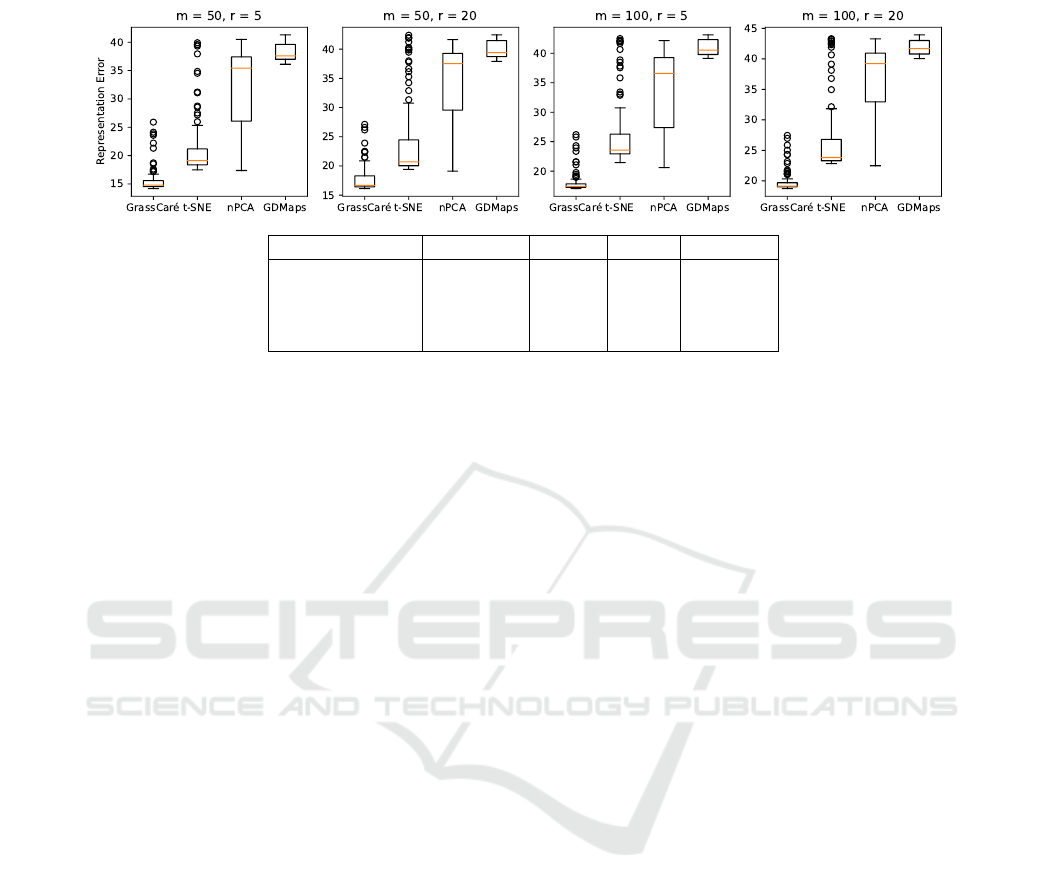
Parameter GrassCaré t-SNE nPCA GDMaps

m = 50;r = 5 59.71s 15.77s 0.04s 0.09s

m = 50;r = 20 59.40s 16.5s 0.03s 0.11s

m = 100;r = 5 60.03s 16.26s 0.03s 0.10s

m = 100;r = 20 77.16 23.10 0.05 0.16

Figure 10: Representation error of GrassCaré (this paper) and other methods for high-dimensional Grassmannians

G(m,r)

The experiments were performed on GoogleColab pro version with cpu.

Visualizing Grassmannians via Poincare Embeddings