False Negative Reduction in Semantic Segmentation Under Domain Shift

Using Depth Estimation

Kira Maag

and Matthias Rottmann

2,3

Ruhr University Bochum, Germany

University of Wuppertal, Germany

EPFL, Switzerland

Keywords:

Deep Learning, Semantic Segmentation, Domain Generalization, Depth Estimation.

Abstract:

State-of-the-Art deep neural networks demonstrate outstanding performance in semantic segmentation. How-

ever, their performance is tied to the domain represented by the training data. Open world scenarios cause

inaccurate predictions which is hazardous in safety relevant applications like automated driving. In this work,

we enhance semantic segmentation predictions using monocular depth estimation to improve segmentation by

reducing the occurrence of non-detected objects in presence of domain shift. To this end, we infer a depth

heatmap via a modiﬁed segmentation network which generates foreground-background masks, operating in

parallel to a given semantic segmentation network. Both segmentation masks are aggregated with a focus on

foreground classes (here road users) to reduce false negatives. To also reduce the occurrence of false positives,

we apply a pruning based on uncertainty estimates. Our approach is modular in a sense that it post-processes

the output of any semantic segmentation network. In our experiments, we observe less non-detected objects

of most important classes and an enhanced generalization to other domains compared to the basic semantic

segmentation prediction.

1 INTRODUCTION

Semantic image segmentation aims at segmenting ob-

jects in an image by assigning each pixel to a class

within a predeﬁned set of semantic classes. Thereby,

semantic segmentation provides comprehensive and

precise information about the given scene. This is

particularly desirable in safety relevant applications

like automated driving. In recent years, deep neu-

ral networks (DNNs) have demonstrated outstanding

performance on this task (Chen et al., 2018; Wang

et al., 2021a). However, DNNs are usually trained

on a speciﬁc dataset (source domain) and often fail to

function properly on unseen data (target domain) due

to a domain gap. In real-world applications, domain

gaps may occur due to shifts in location, time and

other environmental parameters. This causes domain

shift on both, foreground classes – countable objects

such as persons, animals, vehicles – and background

classes – regions with similar texture or material like

sky, road, nature, buildings (Adelson, 2001). Figure 1

gives an example for the lack of generalization, i.e.,

the DNN is trained on street scenes in German cities

(Cordts et al., 2016) resulting in defective behavior

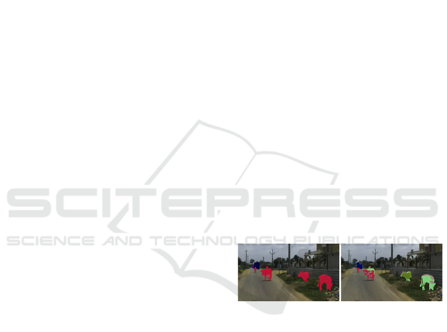
Figure 1: Example image of the India Driving dataset. Left:

Ground truth pixels of classes humans/animals colored in

red and vehicles in blue. Right: Semantic segmentation for

the mentioned classes.

on the unseen India road scenes (Varma et al., 2019)

where the animals are predicted as person, nature or

fence. This is critical since potential hazardous sit-

uations are underestimated due to the prediction of

non-dynamic classes. On the one hand, when us-

ing semantic segmentation in open world scenarios,

the appearance of objects that do not belong to any

of the semantic classes the DNN has been trained on

(like animals) may cause defective predictions (Ping-

gera et al., 2016). On the other hand, even objects of

known classes can change their appearance, leading to

erroneous predictions. Hence, for the deployment of

DNNs in safety-critical applications, robustness un-

der domain shifts is essential.

Maag, K. and Rottmann, M.

False Negative Reduction in Semantic Segmentation Under Domain Shift Using Depth Estimation.

DOI: 10.5220/0011607400003417

In Proceedings of the 18th International Joint Conference on Computer Vision, Imaging and Computer Graphics Theory and Applications (VISIGRAPP 2023) - Volume 5: VISAPP, pages

397-408

ISBN: 978-989-758-634-7; ISSN: 2184-4321

 2023 by SCITEPRESS – Science and Technology Publications, Lda. Under CC license (CC BY-NC-ND 4.0)

397

Unsupervised domain adaptation is an approach

overcoming this issue. The idea is to train a DNN on

labeled source domain data and jointly on unlabeled

target data adapting the source domain distribution to

the target one (Watanabe et al., 2018). As target data

is not always available for training, the recent research

has also been devoted to domain generalization re-

solving this limitation (Lee et al., 2022).

In this work, we introduce a domain generaliza-

tion method for semantic segmentation using depth

estimation focusing on the reduction of false negative

foreground objects. In applications like automated

driving, the foreground class is of particular interest

due to its dynamical behavior. Especially in pres-

ence of domain gaps, the detection performance w.r.t.

these object classes can decrease signiﬁcantly. An

overview of our approach consisting of two branches

(running in parallel) is shown in Figure 2. The im-

age segmentation branch is a semantic segmentation

inference and the depth segmentation branch feeds

the same RGB input image into a depth estimation

network. The goal of depth estimation is to obtain

a representation of the spatial structure of a given

scene, which can help to bridge domain gaps (Wang

et al., 2021b). The resulting depth heatmap is passed

to a modiﬁed segmentation network which predicts

foreground-background segmentation. The architec-

ture of this network may be based on the architec-

ture of the semantic segmentation network, but can be

chosen independently. In the fusion step, the semantic

segmentation and the foreground-background predic-

tion are aggregated obtaining several segments (con-

nected components of pixels belonging to the same

class) per foreground class. As a result of combin-

ing the two masks, we detect overlooked segments

of the basic semantic segmentation network on the

source dataset as well as under domain shift using the

depth information for domain generalization. How-

ever, the increased sensitivity towards ﬁnding fore-

ground objects may result in an overproduction of

false positive segments. To overcome this, we uti-

lize an uncertainty-aware post-processing fusion step,

a so-called meta classiﬁer which performs false pos-

itive pruning with a lightweight classiﬁer (Rottmann

et al., 2020; Maag et al., 2020). Moreover, to gain a

further performance boost, the meta classiﬁer, which

is trained only on the source domain, can be ﬁne-

tuned on a small amount of the respective target do-

main (lightweight domain adaptation).

We only assume input data as well as a trained se-

mantic segmentation and a depth estimation network.

Due to the modularity of our method, we can set up

our model based on these assumptions and it is appli-

cable to any semantic segmentation network i.e., only

the output is post-processed. In our tests, we em-

ploy two semantic segmentation (Chen et al., 2018;

Zhang et al., 2019) and two depth estimation net-

works (Godard et al., 2019; Lee et al., 2019) applied

to four datasets, i.e., Cityscapes (Cordts et al., 2016)

as source domain and A2D2 (Geyer et al., 2020), Lo-

stAndFound (Pinggera et al., 2016) as well as India

Driving (Varma et al., 2019) as target domains. The

application of these widely differing datasets is in-

tended to demonstrate the domain generalization and

error reduction capability of our approach. The source

code is publicly available at http://github.com/kmaag/

FN-Reduction-using-Depth. Our contributions are

summarized as follows:

• We introduce a modiﬁed segmentation network

which is fed with depth heatmaps and out-

puts foreground-background segmentation masks

which are combined with semantic segmentation

masks to detect possible overlooked segments (by

the semantic segmentation network) of the most

important classes. In addition, we perform meta

classiﬁcation to prune false positive segments in

an uncertainty-aware fashion.

• For the ﬁrst time, we demonstrate that incorpo-

rating depth information in a post-processing step

improves a semantic segmentation performance

(independently of the choice of semantic segmen-

tation network). We compare the performance of

our method with basic semantic segmentation per-

formance on several datasets (with domain gap)

obtaining area under precision-recall curve values

of up to 97.08% on source domain and 93.83%

under domain shift.

The paper is structured as follows. In section 2,

we discuss the related work. Our approach is intro-

duced in section 3 including the modiﬁed segmenta-

tion network, the aggregation of network predictions

and meta classiﬁcation. The numerical results are

shown in section 4.

2 RELATED WORK

In this section, we ﬁrst discuss related methods im-

proving robustness of DNNs under domain shift as

well as false negative reduction approaches. There-

after, we present works that use depth information to

enhance semantic segmentation prediction.

Robustness Under Domain Shift. Unsupervised

domain adaptation is often used to strengthen the ro-

bustness of DNNs bridging domain gaps (Watanabe

VISAPP 2023 - 18th International Conference on Computer Vision Theory and Applications

398

RGB input image

depth

estimation

network

modiﬁed

segmentation

network

semantic

segmentation

network

aggregation

meta classiﬁcation

+ evaluation

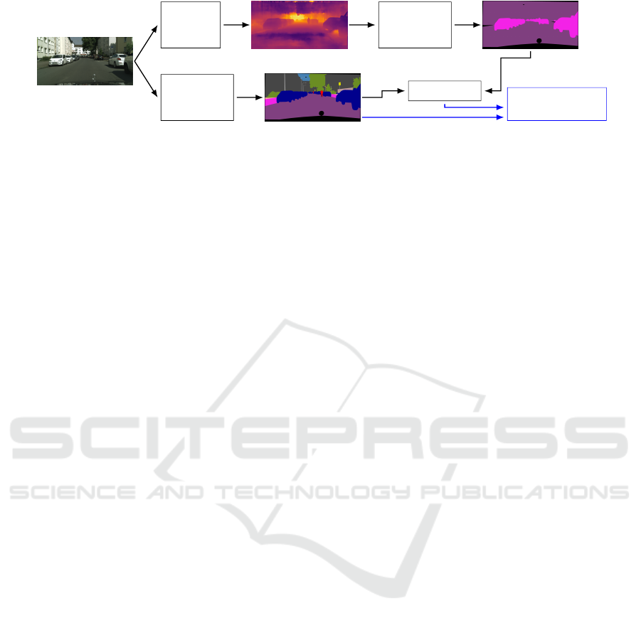
Figure 2: Overview of our method. The input image is fed into a semantic segmentation network (bottom branch) and in

parallel into a depth estimation network (top branch). The resulting depth heatmap is passed to our modiﬁed segmentation

network which predicts a foreground-background segmentation. This prediction is aggregated with the semantic segmentation

and ﬁnally, meta classiﬁcation is applied to reduce false positive segments in an uncertainty-aware manner.

et al., 2018). The DNN is trained with source data (la-

beled) and target data (unlabeled and different from

source dataset) to align the target domain’s distribu-

tions. In (Yan et al., 2019), this problem is tackled

by a generative adversarial network which translates

the target domain into the source domain before pre-

dicting semantic segmentation. Monocular depth es-

timation is used in (Cardace et al., 2022; Wang et al.,

2021b) to improve the prediction performance under

domain shift. However, target data from various en-

vironments is not always available during the train-

ing process. To overcome this limitation, research on

domain generalization has recently gained attention,

using only source data to train the model.

Synthetic to real domain generalization offers a

possibility to exploit the advantage of the availabil-

ity of synthetic data. In (Chen et al., 2020), the syn-

thetically trained network is encouraged to maintain

similar representations as the ImageNet pre-trained

model. In other works, style-diversiﬁed samples

(Zhao et al., 2022) or web-crawled images (Kim et al.,

2021) are utilized for improving the representational

consistency between synthetic and real-world for the

sake of generalizable semantic segmentation. The

model presented in (Shiau et al., 2021) is trained on

multiple source domains (synthetic and real) to gener-

alize to unseen data domains. The variety of contents

and styles from ImageNet is leveraged in (Lee et al.,

2022) to learn domain-generalized semantic features.

In (Choi et al., 2021), an instance selective whitening

loss is introduced to disentangle the domain-speciﬁc

style and domain-invariant content to remove only the

style information causing domain shift.

In contrast to domain adaptation and generaliza-

tion, our method does not require target domain data

or a great amount of source domain data for training,

we only consider depth information for domain gen-

eralization. Moreover, we do not modify the training

process of the semantic segmentation network, i.e.,

we are independent of the network due to modularity.

For these reasons, the presented approaches cannot be

considered as suitable baselines.

False Negative Reduction in Semantic Segmen-

tation. Reducing false negatives, i.e., obtaining a

higher recall rate, is often achieved in semantic seg-

mentation by modifying the loss function. In (Xiang

et al., 2019), a higher recall rate for a real-time DNN

is obtained by modifying the loss function, classiﬁer

and decision rule. A similar approach presented in

(Xiang et al., 2019) considers an importance-aware

loss function to improve a network’s reliability. To re-

duce false negative segments of minority classes, dif-

ferences between the Bayes and the Maximum Like-

lihood decision rule are exploited introducing class

priors that assign larger weight to underrepresented

classes (Chan et al., 2020). Since minority classes are

not necessarily hard to predict, leading to the predic-

tion of many false positives, a hard-class mining loss

is introduced in (Tian et al., 2021) by redesigning the

cross entropy loss to dynamically weight the loss for

each class based on instantaneous recall. In (Zhong

et al., 2021), false negative pixels in semi-supervised

semantic segmentation are reduced by using the pixel-

level ℓ

loss and the pixel contrastive loss.

While the presented approaches modify the train-

ing process and/or the decision rule, we post-process

only the output of the semantic segmentation net-

work. For the ﬁrst time, we present a false negative re-

duction approach which overcomes domain gaps us-

ing depth information. The only work (Maag, 2021)

which also uses depth heatmaps addressing the recall

rate improvement works on video instance segmenta-

tion.

Improving Segmentation Using Depth Estimation.

The predictions of semantic segmentation and depth

estimation masks are improved in previous works us-

ing joint network architectures sharing information

for both tasks (Chen et al., 2019; Jiao et al., 2018).

Furthermore, approaches are introduced where infor-

mation of one task enhance the prediction quality of

the other task. The semantic segmentation task is im-

proved in (Hazirbas et al., 2016) by an encoder con-

False Negative Reduction in Semantic Segmentation Under Domain Shift Using Depth Estimation

399

sisting of two network branches which extract fea-

tures from depth and RGB images simultaneously.

In (Cao et al., 2017), RGB-D data is also fed into a

network that extracts both RGB and depth features

in parallel for semantic segmentation prediction (and

object detection). Contrary, a single shared encoder is

used in (Novosel, 2019) to enhance performance for

a supervised task, here semantic segmentation, which

obtains information of two self-supervised tasks (col-

orization and depth prediction) exploiting unlabeled

data. In (Jiang et al., 2018), a semantic segmentation

network is pre-trained for depth prediction to serve

as a powerful proxy for learning visual representa-

tions. In addition to learning features from depth in-

formation, a student-teacher framework is considered

in (Hoyer et al., 2021) to select the most helpful sam-

ples to annotate for semantic segmentation.

In comparison to the described methods mod-

ifying the network architecture, our foreground-

background prediction runs independently and in

parallel with semantic segmentation inference, and

the aggregation serves as lightweight post-processing

step. In particular, we cannot regard the presented ap-

proaches as suitable baselines since the domain gen-

eralization capability is not tested. However, these

methods demonstrate that depth information can be

used to enhance semantic segmentation.

3 METHOD DESCRIPTION

Our method is composed of two parallel branches,

i.e., the image segmentation and depth segmentation

branch, see Figure 2. The outputs of both streams are

aggregated to detect segments overlooked by the ba-

sic semantic segmentation network. As many false

positive segments can be generated by the fusion,

false positive pruning is applied in an additional post-

processing step.

3.1 Foreground-Background

Segmentation

In this section, we introduce our modiﬁed segmen-

tation network for foreground-background segmenta-

tion. We assume that a depth estimation (and a seman-

tic segmentation ground truth) is available for each in-

put image. Our approach is modular and independent

of the choice of the depth estimation (and the seman-

tic segmentation) network. The basis for the modiﬁed

network can be any standard semantic segmentation

network. However, instead of feeding an RGB im-

age into the network a depth estimation heatmap is

used and the semantic space is composed of only two

classes - foreground and background.

The binarization into foreground and background

is adapted from the thing and stuff decomposition in

the computer vision ﬁeld like in panoptic segmenta-

tion (Kirillov et al., 2019). Using automated driving

as example application, things are countable objects

such as persons, animals, cars or bicycles. The stuff

classes consist of amorphous regions of similar tex-

ture or material such as sky, road, nature or buildings.

Note, the idea of things and stuff also exists in other

application areas like robot navigation.

3.2 Aggregation of Predictions

From the ﬁrst branch, we obtain a semantic segmenta-

tion prediction, i.e., a pixel-wise classiﬁcation of im-

age content. The DNN provides for each pixel z a

probability distribution f

(y|x) over a prescribed label

space y ∈ C = {y

,.. .,y

} with c different class la-

bels, given an input image x. The predicted class for

each pixel z is computed by the maximum a-posteriori

principle

ˆy

(x) = arg max

y∈C

(y|x). (1)

The second branch provides a foreground-

background segmentation. Given the same input

image x, we obtain for each pixel z the probability of

being a foreground pixel g

(x) ∈ [0,1] considering

a binary classiﬁcation problem. The predicted seg-

mentations are aggregated pixel-wise resulting in a

combined prediction with the class label background

or a foreground class label y ∈

C ⊂ C per pixel.

For this, we split the label space into foreground

class labels

C = {y

,... , y

˜c

}, ˜c < c, and background

class labels {y

˜c+1

,... , y

} with y

= C \

C . The

combination is deﬁned per pixel by

ˆs

(x) =











ˆy

(x), if ˆy

(x) ∈

argmax

y∈

(y|x), if g

(x) > 0.5 ∧ ˆy

(x) /∈

, else .

(2)

If the semantic segmentation network predicts a fore-

ground class or the foreground-background network

predicts foreground, the pixel is considered as fore-

ground and assigned to the foreground class y ∈

of the semantic segmentation with the highest prob-

ability. Otherwise, the pixel is assigned to the class

background. Moreover,

= {ˆs

(x)|z ∈ x} denotes

the combined segmentation consisting of foreground

classes and the background class.

VISAPP 2023 - 18th International Conference on Computer Vision Theory and Applications

400

3.3 Meta Classiﬁcation

The combination of the semantic segmentation and

the foreground-background prediction can increase

the number of false positives. For this reason, we ap-

ply meta classiﬁcation (Rottmann et al., 2020) as false

positive pruning step using uncertainty measures. The

degree of randomness in semantic segmentation pre-

diction f

(y|x) is quantiﬁed by (pixel-wise) dispersion

measures, like the entropy. To obtain segment-wise

features characterizing uncertainty of a given segment

from these pixel-wise dispersion measures, we aggre-

gate them over segments by average pooling. In addi-

tion, we hand-craft features based on object’s geom-

etry like the segment size or the geometric center ob-

taining uncertainty information. These hand-crafted

measures form a structured dataset where the rows

correspond to predicted segments and the columns to

features. A detailed description of these hand-crafted

features can be found in Appendix A.

To determine if a predicted segment is a false pos-

itive, i.e., has no overlap with a ground truth seg-

ment of a foreground class, we consider the intersec-

tion over union (IoU, (Jaccard, 1912)), a typical per-

formance measure of segmentation networks with re-

spect to the ground truth. Meta classiﬁcation tackles

the task of classifying between IoU = 0 (false posi-

tive) and IoU > 0 (true positive) for all predicted seg-

ments. If a segment is predicted to be a false positive,

it is no longer considered as a foreground segment but

as background. We perform meta classiﬁcation us-

ing our structured dataset as input. Note, these hand-

crafted measures are computed without the knowl-

edge of the ground truth data. To train the classiﬁer,

we use gradient boosting (Friedman, 2002) that out-

performs linear models and shallow neural networks

as shown in (Maag et al., 2021). We study to which

extent our aggregated prediction followed by meta

classiﬁcation improves the detection performance for

important classes compared to basic semantic seg-

mentation.

4 EXPERIMENTS

In this section, we ﬁrst present the experimental set-

ting and then demonstrate the performance improve-

ments of our method compared to the basic semantic

segmentation network in terms of false negative re-

duction overcoming the domain gap.

4.1 Experimental Setting

Datasets. We perform our tests on four datasets

for semantic segmentation in street scenes consider-

ing Cityscapes (Cordts et al., 2016) as source do-

main and A2D2 (Geyer et al., 2020), LostAnd-

Found (Pinggera et al., 2016) as well as India Driv-

ing (IDD) (Varma et al., 2019) as target domains.

The training/validation split of Cityscapes consists of

2,975/500 images from dense urban trafﬁc in 18/3 dif-

ferent German towns, respectively. Thus, our fore-

ground class consists of all road user classes, i.e., hu-

man (person and rider) and vehicle (car, truck, bus,

train, motorcycle and bicycle) and the background of

categories ﬂat, construction, object, nature and sky.

From the A2D2 dataset, we sample 500 images out

of 23 image sequences for our tests covering urban,

highways and country roads in three cities. This vari-

ety of environments is not included in the Cityscapes

dataset resulting in a domain shift in the background.

The validation set of LostAndFound containing 1,203

images is designed for detecting small obstacles on

the road in front of the ego-car. This causes a fore-

ground domain shift as these objects are not contained

in the semantic space of Cityscapes. We use 538

frames of the IDD dataset which contains unstruc-

tured environments of Indian roads inducing a domain

shift in both, foreground and background. The latter

is caused by, for example, the diversity of ambient

conditions and ambiguous road boundaries. The fore-

ground domain shift occurs as the IDD dataset con-

sists of two more relevant foreground classes (animals

and auto rickshaws) and the Cityscapes foreground

objects differ signiﬁcantly.

Networks. We consider the state-of-the-art

DeepLabv3+ network (Chen et al., 2018) with

WideResNet38 (Wu et al., 2016) as backbone and

the more lightweight (and thus weaker) DualGCNet

(Zhang et al., 2019) with ResNet50 (He et al., 2016)

backbone for semantic segmentation. Both DNNs

are trained on the Cityscapes dataset achieving mean

IoU (mIoU) values of 90.29% for DeepLabv3+

and 79.68% for DualGCNet on the Cityscapes

validation set. For depth estimation trained on the

KITTI dataset (Geiger et al., 2013), we use the

supervised depth estimation network BTS (Lee

et al., 2019) with DenseNet-161 (Huang et al., 2017)

backbone obtaining a relative absolute error on the

KITTI validation set of 0.090 and the unsupervised

Monodepth2 (Godard et al., 2019) with ResNet18

backbone achieving 0.106 relative absolute error.

Our modiﬁed segmentation network is based on

the DeepLabv3+ architecture with WideResNet38

False Negative Reduction in Semantic Segmentation Under Domain Shift Using Depth Estimation

401

backbone having high predictive power and is fed

with depth estimation heatmaps of the Cityscapes

dataset predicted by the BTS network and Mon-

odepth2, respectively. We train this network on the

training split of the Cityscapes dataset and use the

binarized (into foreground and background) semantic

segmentation ground truth to compare our results

with the basic semantic segmentation network which

is also trained on Cityscapes. For the BTS network

a validation mIoU of 88.34% is obtained and for

Monodepth2 of 85.12%.

Evaluation Metrics. Meta classiﬁcation provides

a probability of observing a false positive seg-

ment and such a predicted false positive segment

is considered as background. We threshold on

this probability with 101 different values h ∈ H =

{0.00,0.01,... , 0.99,1.00}. For each threshold, we

calculate the number of true positive, false posi-

tive and false negative foreground segments result-

ing in precision (prec(h)) and recall (rec(h)) val-

ues on segment-level depended of h. The degree

of separability is then computed as the area under

precision recall curve (AUPRC) by thresholding the

meta classiﬁcation probability. In addition, we com-

pute the recall rate at 80% precision rate (REC

)

for the evaluation. Furthermore, we consider the

segment-wise F

score which is deﬁned by F

(h) =

2 · prec(h) · rec(h)/(prec(h) + rec(h)). To obtain an

evaluation metric independent of the meta classiﬁca-

tion threshold h, we calculate the averaged F

score

|H|

∑

h∈H

(h) and the optimal F

score F

∗

max

h∈H

(h). For a detailed description of these

metrics see Appendix B.

4.2 Numerical Results

Results on the Source Domain. First, we study the

predictive power of the meta classiﬁer trained on the

Cityscapes (validation) dataset using a train/test split-

ting of 80%/20% shufﬂing 5 times, such that all seg-

ments are a part of the test set. We use meta classi-

ﬁcation to prune possible false positive segments that

are falsely predicted as foreground segments. For the

comparison of basic semantic segmentation perfor-

mance with our approach, meta classiﬁers are trained

on the predicted foreground segments, respectively.

These classiﬁers achieve test classiﬁcation AUROC

values between 94.68% and 99.14%. The AUROC

(area under receiver operating characteristic curve) is

obtained by varying the decision threshold in a binary

classiﬁcation problem, here for the decision between

IoU = 0 and > 0. The inﬂuence of meta classiﬁcation

on the performance is studied in Appendix C.

Table 1: Performance results for the Cityscapes dataset

for the basic semantic segmentation prediction vs. our ap-

proach, i.e., the DeepLabv3+/DualGCNet prediction aggre-

gated with foreground-background prediction using BTS or

Monodepth2.

AUPRC

∗

REC

DeepLabv3+ 94.26 90.61 94.69 94.49

+ BTS 97.07 90.21 95.80 97.15

+ Monodepth2 97.08 90.03 95.73 97.15

DualGCNet 91.85 88.68 92.77 92.18

+ BTS 95.90 87.92 94.66 95.88

+ Monodepth2 95.63 87.94 94.58 95.66

Table 2: mIoU results for both semantic segmentation net-

works and the difference to our approach. A higher mIoU

value corresponds to better performance.

Cityscapes A2D2 IDD

DeepLabv3+ 90.29% 61.98% 57.26%

+ BTS −4.72 pp −2.87 pp −1.59 pp

+ Monodepth2 −5.97 pp −4.84 pp −3.99 pp

DualGCNet 79.68% 23.76% 45.79%

+ BTS −3.99 pp +0.12 pp −1.03 pp

+ Monodepth2 −5.09 pp −0.49 pp −3.12 pp

We compare the detection performances which are

shown in Table 1 using presented evaluation metrics.

We observe that our method obtain higher AUPRC,

∗

and REC

values than the semantic segmentation

prediction. Note, there is no consistency on which

depth estimation network yields more enhancement.

In particular, we reduce the number of non-detected

segments of foreground classes. In Figure 3 (left),

the highest recall values of the semantic segmentation

predictions are shown, i.e., no segments are deleted

using meta classiﬁcation. For our method, we use

the meta classiﬁcation threshold where the precision

of our method is equal to that of the baseline. As a

consequence, for the identical precision values we ob-

verse an increase in recall by up to 2.71 percent points

(pp) for the Cityscapes dataset. In Appendix D, more

numerical results evaluated on individual foreground

classes are presented.

The mIoU is the commonly used performance

measure for semantic segmentation. To compute the

mIoU for the aggregated prediction

, we have to ﬁll

the background values as they are ignored up to now.

Similar to how we obtain the foreground class dur-

ing the combination, we assign to every background

pixel the background class y ∈ C \

C of the semantic

segmentation with the highest probability. The results

for semantic segmentation prediction and the differ-

ence to our aggregated predictions are shown in the

Cityscapes column of Table 2. We perform slightly

worse in the overall performance accuracy (mIoU) as

the foreground-background masks are location-wise

less accurate than the segmentation masks, see Fig-

ure 4. The reason is that the modiﬁed segmentation

network is fed with predicted depth heatmaps which

VISAPP 2023 - 18th International Conference on Computer Vision Theory and Applications

402

Figure 3: Left: The recall values under the assumption of same precision values for all datasets and networks. We distinguish

the performance for the DeepLabv3+ (DL) and the DualGCNet (DG) semantic segmentation networks whose predictions

serve as baselines. We compare these with our approach using the BTS and the Monodepth2 depth estimation network,

respectively. Center: Precision-recall curves for the A2D2 dataset, the DeepLabv3+ and BTS networks. Right: Number of

false positive vs. false negative segments for different meta classiﬁcation thresholds for the IDD dataset, the DualGCNet and

BTS networks using 20% of this dataset for ﬁne-tuning.

may be inaccurate resulting in less precise separation

of foreground and background. Nonetheless, we de-

tect foreground objects, here road users, that are over-

looked by the semantic segmentation network (for ex-

ample, see the bicycle in Figure 4 (left)).

Results Under Domain Shift. In this section, we

study the false negative reduction for the A2D2, Lo-

stAndFound and IDD datasets under domain shift

from the source domain Cityscapes. As mentioned

above, since the semantic segmentation networks

as well as the modiﬁed segmentation networks are

trained on the Cityscapes dataset, we train also the

meta classiﬁcation model on this dataset using all pre-

dicted segments. We obtain meta classiﬁcation test

AUROC values up to 93.12% for A2D2, 91.65% for

LostAndFound and 93.97% for IDD.

We compare the performance of our approach

with the semantic segmentation prediction by com-

puting the evaluation metrics, results are given in Ta-

ble 3. The performance metrics are greatly increased

by our method demonstrating that our approach is

more robust to domain shift. Noteworthy, we outper-

form the stronger DeepLabv3+ network in all cases.

Example curves are presented in Figure 3 (center) for

the A2D2 dataset where an AUPRC enhancement of

11.45 pp is obtained. Our precision-recall curve is

entirely above the baseline. In particular, for identical

precision values, we obtain an increase in recall by

up to 13.24 pp, i.e., reduce the number of false neg-

ative segments, as also shown in Figure 3 (left). Ex-

amples for detected segments that are missed by the

semantic segmentation network are given in Figure 4

for all datasets. Hence, our method detect segments

of well-trained classes, i.e., the overlooked bicycle in

the Cityscapes dataset or various cars in A2D2. More-

over, we bridge the domain gap as we ﬁnd small ob-

stacles (LostAndFound) and animals (IDD) that are

not part of the Cityscapes dataset and thus, are not

included in the semantic space for training. In Ap-

pendix D, more numerical results evaluated on indi-

vidual foreground classes are presented.

In Table 2, the differences between the mIoU val-

ues are evaluated on the Cityscapes classes. For

the A2D2 dataset, the classes are mapped to the

Cityscapes ones and for the IDD dataset, we treat the

additional classes animal as human and auto rickshaw

as car. For the LostAndFound, an evaluation is not

possible as it contains only labels for the road and

the small obstacles which do not ﬁt into the semantic

space. With one positive exception, we are slightly

worse in overall accuracy performance. On the one

hand, the images in Figure 4 demonstrate why we de-

crease the accuracy slightly as the predictions and in

particular, the segment boundaries are less accurate.

On the other hand, these images motivate the beneﬁt

of our method as completely overlooked segments are

detected. Furthermore, we bridge the domain shift in

a post-processing manner that only requires two more

inferences which run in parallel to semantic segmen-

tation prediction.

Fine-Tuning of the Meta Classiﬁer. Up to now,

we have trained the segmentation networks as well as

the meta classiﬁer on Cityscapes for the experiments

on A2D2, LostAndFound and IDD dataset. In this

paragraph, we investigate the predictive power of the

meta classiﬁer and the implications on false negative

reduction using parts of the target dataset for ﬁne-

tuning. Note, this domain adaptation only occurs in

the post-processing meta classiﬁcation step (retrain-

ing the neural networks is not necessary) and thus, the

ﬁne-tuning is lightweight and requires only a small

amount of ground truth data. In detail, we retrain the

meta classiﬁer with 20%, 40%, 60% and 80% of the

target dataset, respectively. The corresponding per-

False Negative Reduction in Semantic Segmentation Under Domain Shift Using Depth Estimation

403

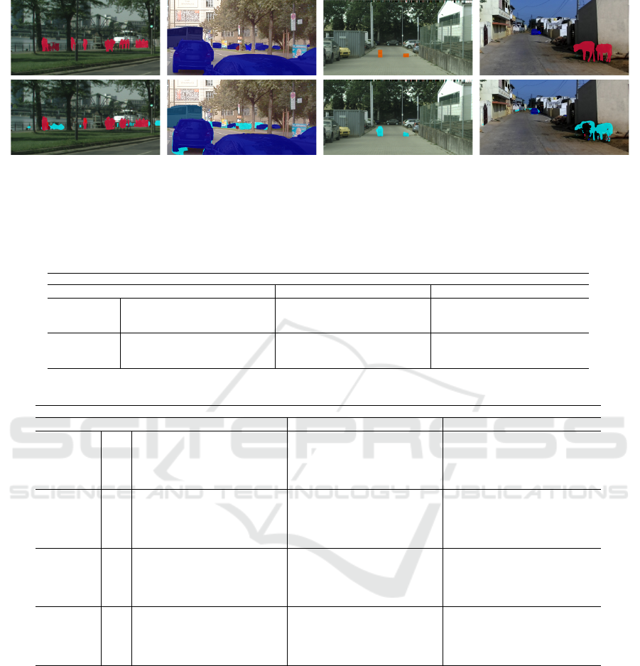
Figure 4: Examples for segments that are overlooked by the basic semantic segmentation network and detected by our ap-

proach for Cityscapes (DualGCNet, BTS, left), A2D2 (DeepLabv3+, BTS, center left), LostAndFound (DeepLabv3+, Mon-

odepth2, center right) and IDD dataset (DeepLabv3+, BTS, right). Top: Ground truth images including only the labels of

foreground classes. Bottom: Basic semantic segmentation prediction in typical Cityscapes colors for foreground segments

(shades of blue and red) as well as the foreground prediction of our modiﬁed segmentation network (cyan).

Table 3: Performance results for the basic semantic segmentation prediction vs. our approach.

A2D2 LostAndFound IDD

AUPRC

∗

REC

AUPRC

∗

REC

AUPRC

∗

REC

DeepLabv3+ 68.74 52.72 76.36 70.80 40.05 50.27 53.06 39.40 84.11 69.19 87.79 88.52

+ BTS 80.19 66.96 80.46 77.17 46.18 51.08 57.80 45.06 93.86 78.48 91.75 93.26

+ Monodepth2 80.01 66.77 80.72 77.15 51.67 54.15 60.41 48.07 93.35 76.69 91.45 92.86

DualGCNet 48.64 27.93 65.48 58.67 36.80 45.85 50.21 36.08 84.59 66.40 87.37 88.20

+ BTS 42.16 36.27 51.22 26.90 42.34 47.27 53.59 40.12 92.23 71.85 89.78 92.53

+ Monodepth2 49.03 39.01 57.26 19.29 47.92 49.11 57.06 44.16 92.39 73.17 89.82 92.23

Table 4: Evaluation results obtained by different splittings that are used for ﬁne-tuning the meta classiﬁer.

A2D2 LostAndFound IDD

AUPRC

∗

REC

AUPRC

∗

REC

AUPRC

∗

REC

0% 80.19 66.96 80.46 77.17 46.18 51.08 57.80 45.06 93.86 78.48 91.75 93.26

DeepLabv3+ 20% 83.65 75.90 85.13 82.01 48.79 60.30 63.57 48.92 94.65 82.12 93.24 93.85

+ 40% 83.72 76.03 85.25 82.25 49.01 60.89 64.01 49.04 94.66 82.24 93.46 93.79

BTS 60% 83.75 75.99 85.39 82.05 49.11 61.41 64.67 49.16 94.86 82.19 93.43 93.89

80% 83.67 75.89 85.50 82.27 48.88 61.33 64.53 49.28 94.67 82.23 93.42 93.93

0% 80.01 66.77 80.72 77.15 51.67 54.15 60.41 48.07 93.35 76.69 91.45 92.86

DeepLabv3+ 20% 82.91 76.00 85.02 81.79 55.77 63.70 68.58 55.72 94.16 81.24 92.58 93.48

+ 40% 83.12 76.23 84.98 82.18 56.19 64.44 69.25 56.14 94.21 81.36 92.69 93.59

Monodepth2 60% 83.10 76.11 85.19 81.96 56.06 64.57 69.58 56.20 94.19 81.41 92.65 93.47

80% 83.03 75.94 85.15 81.68 56.11 64.50 69.65 56.39 94.17 81.31 92.50 93.49

0% 42.16 36.27 51.22 26.90 42.34 47.27 53.59 40.12 92.23 71.85 89.78 92.53

DualGCNet 20% 82.59 74.59 83.06 80.56 45.76 56.88 60.12 45.48 94.71 81.85 92.56 93.79

+ 40% 82.85 74.83 83.82 81.26 46.15 58.08 61.24 46.14 94.74 81.99 92.75 93.70

BTS 60% 82.82 74.72 83.58 81.20 46.19 58.15 61.26 46.39 94.71 81.85 92.73 93.77

80% 82.76 74.53 83.53 81.20 46.24 58.53 61.82 46.27 94.67 81.85 92.65 93.68

0% 49.03 39.01 57.26 19.29 47.92 49.11 57.06 44.16 92.39 73.17 89.82 92.23

DualGCNet 20% 81.98 74.66 83.26 80.69 53.14 61.26 65.97 53.01 94.27 81.56 91.93 93.31

+ 40% 82.27 74.97 83.28 81.02 53.77 62.30 66.95 53.61 94.39 81.60 92.02 93.51

Monodepth2 60% 82.31 75.14 83.34 81.35 53.91 62.48 67.17 53.80 94.40 81.64 92.32 93.31

80% 82.06 74.42 82.91 80.82 53.76 62.59 67.21 53.73 94.34 81.54 91.96 93.47

formance results are shown in Table 4.

We observe great enhancements even with only a

ﬁne-tuning of 20% of the target domain obtaining an

increase of up to 40.43 pp for AUPRC. The maxi-

mal increase is achieved for the A2D2 dataset (on the

DualGCNet and BTS networks) for which 20% corre-

spond to about 100 images that are used for retraining

and achieving such an improvement. For all datasets,

the greatest performance gap occurs between a trained

meta classiﬁer only on the Cityscapes dataset and us-

ing a small amount of the target domain data (here

20%). Increasing the subset of the target data, the

performance is only slightly enhanced. Using 20%

for ﬁne-tuning, the highest AUPRC value of 94.71%

is obtained by the DualGCNet and the BTS network

on the IDD dataset. The corresponding number of

false positives and false negatives is given in Figure 3

(right). Note, the meta classiﬁer for the baseline pre-

diction is trained on the same train splitting. We out-

perform the basic semantic segmentation prediction

and thus achieve a lower number of detection errors,

in particular false negatives, therefore bridging the

domain gap.

VISAPP 2023 - 18th International Conference on Computer Vision Theory and Applications

404

5 CONCLUSION

In this work, we proposed a domain generalization

method applicable to any semantic segmentation net-

work using monocular depth estimation, in particu-

lar reducing non-detected segments. We inferred a

depth heatmap via a modiﬁed segmentation network

that predicts foreground-background masks in paral-

lel to a semantic segmentation network. Aggregat-

ing both predictions in an uncertainty-aware manner

with a focus on important classes, false negative seg-

ments were successfully reduced. Our experiments

suggest that also in a single-sensor setup, the informa-

tion about spatial structure from pre-trained monocu-

lar depth estimators can be utilized well to improve

the robustness of off-the-shelf segmentation networks

under domain shift in various settings.

ACKNOWLEDGEMENTS

We thank M. K. Neugebauer for support in data han-

dling and programming. This work is supported by

the Ministry of Culture and Science of the German

state of North Rhine-Westphalia as part of the KI-

Starter research funding program.

REFERENCES

Adelson, E. H. (2001). On seeing stuff: the perception of

materials by humans and machines. In IS&T/SPIE

Electronic Imaging. 1

Cao, Y., Shen, C., and Shen, H. T. (2017). Exploiting

depth from single monocular images for object detec-

tion and semantic segmentation. IEEE Transactions

on Image Processing. 4

Cardace, A., Luigi, L., Zama Ramirez, P., Salti, S., and

Di Stefano, L. (2022). Plugging self-supervised

monocular depth into unsupervised domain adaptation

for semantic segmentation. 3

Chan, R., Rottmann, M., H

uger, F., Schlicht, P., and

Gottschalk, H. (2020). Metafusion: Controlled false-

negative reduction of minority classes in semantic seg-

mentation. IEEE International Joint Conference on

Neural Networks (IJCNN). 3

Chen, L.-C., Zhu, Y., Papandreou, G., Schroff, F., and

Adam, H. (2018). Encoder-decoder with atrous sep-

arable convolution for semantic image segmentation.

In European Conference on Computer Vision (ECCV).

1, 2, 5

Chen, P.-Y., Liu, A. H., Liu, Y.-C., and Wang, Y.-C. F.

(2019). Towards scene understanding: Unsupervised

monocular depth estimation with semantic-aware rep-

resentation. In IEEE/CVF Conference on Computer

Vision and Pattern Recognition (CVPR). 3

Chen, W., Yu, Z., Wang, Z., and Anandkumar, A. (2020).

Automated synthetic-to-real generalization. In Inter-

national Conference on Machine Learning (ICML). 3

Choi, S., Jung, S., Yun, H., Kim, J. T., Kim, S., et al.

(2021). Robustnet: Improving domain generalization

in urban-scene segmentation via instance selective

whitening. IEEE/CVF Conference on Computer Vi-

sion and Pattern Recognition (CVPR), pages 11575–

11585. 3

Cordts, M., Omran, M., Ramos, S., Rehfeld, T., Enzweiler,

M., et al. (2016). The cityscapes dataset for semantic

urban scene understanding. In IEEE Conference on

Computer Vision and Pattern Recognition (CVPR). 1,

2, 5, 12

Friedman, J. H. (2002). Stochastic gradient boosting. Com-

put. Stat. Data Anal. 5

Geiger, A., Lenz, P., Stiller, C., and Urtasun, R. (2013).

Vision meets robotics: The kitti dataset. The Interna-

tional Journal of Robotics Research. 5

Geyer, J., Kassahun, Y., Mahmudi, M., Ricou, X., Durgesh,

R., et al. (2020). A2D2: Audi Autonomous Driving

Dataset. 2, 5, 12

Godard, C., Mac Aodha, O., Firman, M., and Brostow, G. J.

(2019). Digging into self-supervised monocular depth

prediction. 2, 5

Hazirbas, C., Ma, L., Domokos, C., and Cremers, D.

(2016). Fusenet: Incorporating depth into semantic

segmentation via fusion-based cnn architecture. In

Asian Conference on Computer Vision (ACCV). 3

He, K., Zhang, X., Ren, S., and Sun, J. (2016). Deep resid-

ual learning for image recognition. 5

Hoyer, L., Dai, D., Chen, Y., Koring, A., Saha, S., et al.

(2021). Three ways to improve semantic segmentation

with self-supervised depth estimation. 4

Huang, G., Liu, Z., and Weinberger, K. Q. (2017). Densely

connected convolutional networks. IEEE Conference

on Computer Vision and Pattern Recognition (CVPR).

Jaccard, P. (1912). The distribution of the ﬂora in the alpine

zone. New Phytologist. 5

Jiang, H., Larsson, G., Maire, M., Shakhnarovich, G., and

Learned-Miller, E. G. (2018). Self-supervised relative

depth learning for urban scene understanding. In Eu-

ropean Conference on Computer Vision (ECCV). 4

Jiao, J., Cao, Y., Song, Y., and Lau, R. (2018). Look deeper

into depth: Monocular depth estimation with semantic

booster and attention-driven loss. In European Con-

ference on Computer Vision (ECCV). 3

Kim, N., Son, T., Lan, C., Zeng, W., and Kwak, S. (2021).

Wedge: Web-image assisted domain generalization

for semantic segmentation. 3

Kirillov, A., He, K., Girshick, R., Rother, C., and Dollar, P.

(2019). Panoptic segmentation. In IEEE/CVF Con-

ference on Computer Vision and Pattern Recognition

(CVPR). 4

Lee, J. H., Han, M.-K., Ko, D. W., and Suh, I. H. (2019).

From big to small: Multi-scale local planar guidance

for monocular depth estimation. 2, 5

Lee, S., Seong, H., Lee, S., and Kim, E. (2022). Wildnet:

False Negative Reduction in Semantic Segmentation Under Domain Shift Using Depth Estimation

405

Learning domain generalized semantic segmentation

from the wild. 2, 3

Maag, K. (2021). False negative reduction in video instance

segmentation using uncertainty estimates. In IEEE In-

ternational Conference on Tools with Artiﬁcial Intel-

ligence (ICTAI). 3

Maag, K., Rottmann, M., and Gottschalk, H. (2020). Time-

dynamic estimates of the reliability of deep semantic

segmentation networks. In IEEE International Con-

ference on Tools with Artiﬁcial Intelligence (ICTAI).

Maag, K., Rottmann, M., Varghese, S., H

uger, F., Schlicht,

P., et al. (2021). Improving video instance segmen-

tation by light-weight temporal uncertainty estimates.

In International Joint Conference on Neural Network

(IJCNN). 5

Novosel, J. (2019). Boosting semantic segmentation with

multi-task self-supervised learning for autonomous

driving applications. 4

Pinggera, P., Ramos, S., Gehrig, S., Franke, U., Rother, C.,

et al. (2016). Lost and found: detecting small road

hazards for self-driving vehicles. In IEEE/RSJ Inter-

national Conference on Intelligent Robots and Sys-

tems (IROS). 1, 2, 5

Rottmann, M., Colling, P., Hack, T., H

uger, F., Schlicht, P.,

et al. (2020). Prediction error meta classiﬁcation in

semantic segmentation: Detection via aggregated dis-

persion measures of softmax probabilities. In IEEE

International Joint Conference on Neural Networks

(IJCNN) 2020. 2, 5

Shiau, Z.-Y., Lin, W.-W., Lin, C.-S., and Wang, Y.-C. F.

(2021). Meta-learned feature critics for domain gen-

eralized semantic segmentation. 3

Tian, J., Mithun, N. C., Seymour, Z., Chiu, H., and Kira,

Z. (2021). Striking the right balance: Recall loss for

semantic segmentation. 3

Varma, G., Subramanian, A., Namboodiri, A., Chandraker,

M., and Jawahar, C. (2019). Idd: A dataset for ex-

ploring problems of autonomous navigation in uncon-

strained environments. In IEEE Winter Conf. on Ap-

plications of Computer Vision (WACV). 1, 2, 5, 12

Wang, J., Sun, K., Cheng, T., Jiang, B., Deng, C., et al.

(2021a). Deep high-resolution representation learning

for visual recognition. IEEE Transactions on Pattern

Analysis and Machine Intelligence. 1

Wang, Q., Dai, D., Hoyer, L., Van Gool, L., and Fink,

O. (2021b). Domain adaptive semantic segmentation

with self-supervised depth estimation. In IEEE/CVF

International Conference on Computer Vision (ICCV).

2, 3

Watanabe, K., Saito, K., Ushiku, Y., and Harada, T. (2018).

Multichannel semantic segmentation with unsuper-

vised domain adaptation. European Conference on

Computer Vision (ECCV) Workshop. 2, 3

Wu, Z., Shen, C., and Hengel, A. (2016). Wider or deeper:

Revisiting the resnet model for visual recognition.

Pattern Recognition. 5

Xiang, K., Wang, K., and Yang, K. (2019). A compara-

tive study of high-recall real-time semantic segmen-

tation based on swift factorized network. Security +

Defence. 3

Xiang, K., Wang, K., and Yang, K. (2019). Importance-

aware semantic segmentation with efﬁcient pyrami-

dal context network for navigational assistant systems.

IEEE Intelligent Transportation Systems Conference

(ITSC). 3

Yan, W., Wang, Y., Gu, S., Huang, L., Yan, F., et al. (2019).

The domain shift problem of medical image segmen-

tation and vendor-adaptation by unet-gan. Medical

Image Computing and Computer Assisted Interven-

tion. 3

Zhang, L., Li, X., Arnab, A., Yang, K., Tong, Y., et al.

(2019). Dual graph convolutional network for seman-

tic segmentation. In British Machine Vision Confer-

ence (BMVC). 2, 5

Zhao, Y., Zhong, Z., Zhao, N., Sebe, N., and Lee, G. H.

(2022). Style-hallucinated dual consistency learning

for domain generalized semantic segmentation. 3

Zhong, Y., Yuan, B., Wu, H., Yuan, Z., Peng, J., et al.

(2021). Pixel contrastive-consistent semi-supervised

semantic segmentation. In IEEE/CVF International

Conference on Computer Vision (ICCV). 3

APPENDIX

A Details on Meta Classiﬁcation

The semantic segmentation neural network provides

for each pixel z a probability distribution f

(y|x) over

a label space C = {y

,... , y

}, with y ∈ C and given an

input image x. The degree of randomness in semantic

segmentation prediction is quantiﬁed by (pixel-wise)

dispersion measures, such as the entropy

(x) = −

log(c)

∑

y∈C

(y|x)log f

(y|x), (3)

(see Figure 5 (right)) the variation ratio

= 1 − f

( ˆy

(x)|x) (4)

or the probability margin

(x) = V

+ max

y∈C \{ ˆy

(x)}

(y|x) (5)

with predicted class ˆy

(x) (see Equation 1). Based

on the different behavior of these measures and the

segment’s geometry for correct and false predictions,

we construct segment-wise features by hand to quan-

tify the observations that we made. Let

denote

the set of predicted segments, i.e., connected compo-

nents, (of the foreground class). By aggregating these

pixel-wise measures, segment-wise features are ob-

tained and serve as input for the meta classiﬁer. To

this end, we compute for each segment q ∈

the

mean of the pixel-wise uncertainty values of a given

segment, i.e., mean dispersions

D, D ∈ {E,V,M}.

Furthermore, we distinguish between the inner of the

VISAPP 2023 - 18th International Conference on Computer Vision Theory and Applications

406

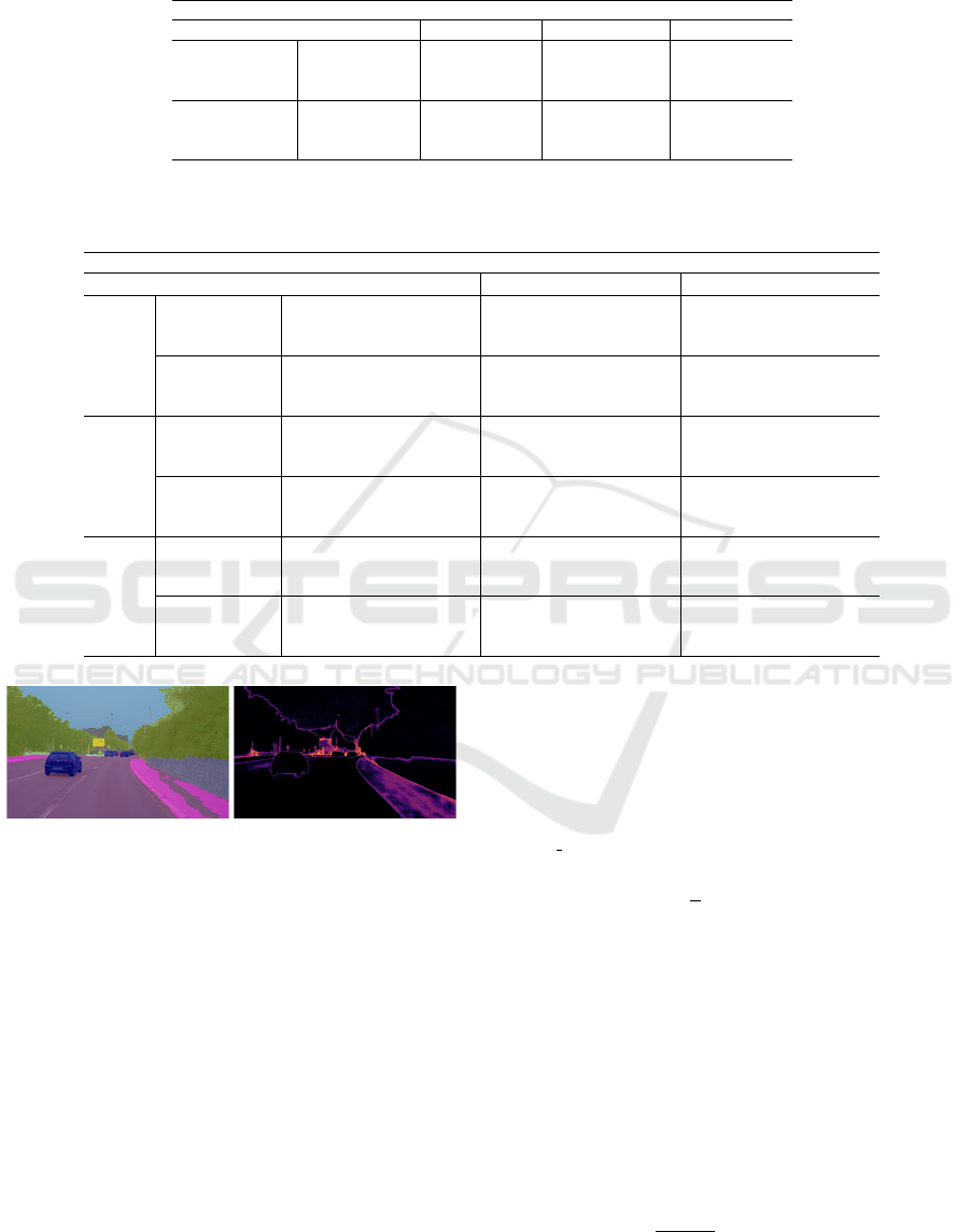
Table 5: Evaluation results using meta classiﬁcation (F

∗

) and without (F

(1)) for the basic semantic segmentation predic-

tion (DeepLabv3+/DualGCNet) and our approach, i.e., the DeepLabv3+/DualGCNet prediction aggregated with foreground-

background prediction using BTS or Monodepth2.

Cityscapes A2D2 LostAndFound IDD

(1) F

∗

(1) F

∗

(1) F

∗

(1) F

∗

DeepLabv3+ 84.00 94.69 52.16 76.36 49.54 53.06 69.14 87.79

+ BTS 43.16 95.80 25.09 80.46 40.19 57.80 39.00 91.75

+ Monodepth2 38.11 95.73 17.16 80.72 33.61 60.41 25.73 91.45

DualGCNet 82.82 92.77 25.89 65.48 45.88 50.21 64.11 87.37

+ BTS 53.99 94.66 25.40 51.22 40.17 53.59 44.64 89.78

+ Monodepth2 50.92 94.58 23.98 57.26 35.07 57.06 35.87 89.82

Table 6: Performance results for the basic semantic segmentation prediction (DeepLabv3+/DualGCNet) vs. our approach,

i.e., the DeepLabv3+/DualGCNet prediction aggregated with foreground-background prediction using BTS or Monodepth2,

for class person, car and bicycle.

Cityscapes A2D2 IDD

AUPRC

∗

AUPRC

∗

AUPRC

∗

person DeepLabv3+ 83.11 80.33 84.66 40.66 40.19 54.83 39.70 35.31 56.78

+ BTS 87.36 80.36 86.89 47.10 43.37 55.43 46.14 41.05 54.94

+ Monodepth2 86.87 80.27 86.62 48.85 41.83 56.60 48.88 40.73 56.80

DualGCNet 75.05 73.30 77.12 13.67 17.64 35.34 31.29 25.37 47.28

+ BTS 79.72 73.24 80.30 13.28 20.68 28.42 36.94 30.23 47.72

+ Monodepth2 78.39 72.78 79.70 13.56 21.28 28.61 41.51 31.48 48.08

car DeepLabv3+ 86.19 85.18 89.31 64.77 56.21 73.16 55.25 39.92 70.03

+ BTS 89.20 85.69 90.61 75.53 66.74 77.44 69.99 50.97 73.45

+ Monodepth2 88.83 85.15 90.20 74.82 67.26 77.45 68.03 49.70 72.59

DualGCNet 81.76 81.45 85.44 39.65 21.93 59.85 57.28 41.89 69.07

+ BTS 85.88 81.31 87.39 33.52 30.37 46.14 63.12 46.67 69.70

+ Monodepth2 85.24 81.24 87.13 40.63 34.00 53.89 64.52 48.50 69.93

bicycle DeepLabv3+ 85.46 80.25 87.43 37.37 47.00 49.67 14.36 9.73 33.73

+ BTS 86.99 79.02 86.64 43.78 48.47 54.88 21.70 13.70 38.25

+ Monodepth2 87.20 78.54 86.93 42.37 46.97 53.24 23.78 13.79 39.84

DualGCNet 77.05 73.43 80.62 15.22 19.85 27.27 16.06 8.68 36.79

+ BTS 79.49 72.68 81.16 8.08 21.30 23.08 16.00 9.56 33.51

+ Monodepth2 79.99 72.82 81.93 10.23 19.70 21.28 21.93 10.70 36.36

Figure 5: Left: Semantic segmentation predicted by a DNN.

Right: Entropy heatmap.

segment q

⊂ q consisting of all pixels whose eight

neighboring pixels are also elements of q and the

boundary q

= q \ q

. We observe that poor or false

predictions are often accompanied by fractal segment

shapes (a relatively large amount of boundary pixels).

An example is shown in Figure 5 (left). This results

in segment size S = |q| and mean dispersion features

per segment also for the inner and the boundary since

uncertainties may be higher on a segment’s bound-

ary (see Figure 5 (right)). Additionally, we deﬁne

relative segment sizes

S = S/S

and

= S

quantifying the degree of fractality as well as rela-

tive mean dispersions

D =

S and

where

D ∈ {E,V,M}.

For the foreground-background segmentation,

given the same input image x, we obtain for each

pixel z the probability of being a foreground pixel

(x) ∈ [0,1]. Thus, we calculate the mean and rel-

ative entropy features for the foreground-background

prediction (having only two classes), denoted by

∗

∗ ∈ { ,in, bd},

F and

. Last, we add the geometric

center

¯q =

∑

)∈q

) (6)

where (z

) describes the vertical and horizontal co-

ordinate of pixel z and the mean class probabilities

P(y|q) for each foreground class y ∈

C ⊂ C where

C = {y

,... , y

˜c

}, ˜c < c, to our set of hand-crafted fea-

tures.

Analogously to the set of predicted segments

we denote by P

the set of segments in the ground

truth S

. To determine if a predicted segment q ∈

is a false positive, we consider the intersection over

union. The segment-wise IoU is then deﬁned as

IoU(q) =

|q ∩ Q|

|q ∪ Q|

, Q =

[

′

∈P

′

∩q̸=

′

. (7)

False Negative Reduction in Semantic Segmentation Under Domain Shift Using Depth Estimation

407

B More Details on Evaluation

Metrics

Let

denote the set of predicted segments and P

ground truth segments. Meta classiﬁcation provides a

probability m(q) ∈ [0,1] for each segment q ∈

to be

a false positive on which we threshold with different

values h ∈ H = {0.00,0.01,... , 0.99,1.00}. A pre-

dicted false positive segment is considered as back-

ground. For each threshold h, we calculate over of all

foreground segments in a given validation set X the

number of false positives

FP(h) =

∑

x∈X

∑

q∈

{IoU(q)=0}

{m(q)≤h}

, (8)

true positives

TP(h) =

∑

x∈X

∑

′

∈P

{IoU

′

(q,h)>0}

(9)

and false negatives

FN(h) =

∑

x∈X

∑

′

∈P

{IoU

′

(q,h)=0}

(10)

where the indicator function is deﬁned as

{A}

(

1, if event A happens

0, else

(11)

and the IoU for a ground truth segment q

′

∈ P

IoU

′

,h) =

′

∩ Q

′

∪ Q

′

, Q

′

[

q∈

,q∩q

′

̸=

m(q)≤h

q. (12)

Thus, we obtain precision, prec(h) =

TP(h)/(TP(h) + FP(h)), and recall, rec(h) =

TP(h)/(TP(h) + FN(h)), values on segment-level

dependent of h. The degree of separability is then

computed as the area under precision recall curve

(AUPRC) by thresholding the meta classiﬁcation

probability. Furthermore, we use the recall rate

at 80% precision rate (REC

) for the evaluation.

Moreover, we consider the segment-wise F

score

which is deﬁned by

(h) = 2 ·

prec(h) · rec(h)

prec(h) + rec(h)

. (13)

To obtain an evaluation metric independent of the

meta classiﬁcation threshold h, we calculate the aver-

aged F

score

= 1/|H|

∑

h∈H

(h) and the optimal

score F

∗

= max

h∈H

(h).

C Effects of Meta Classiﬁcation

In Table 5, we show the effects of meta classiﬁca-

tion comparing the F

score (see Equation 13) per-

formance with and without meta classiﬁcation. F

(1)

corresponds to the obtained precision and recall val-

ues without post-processing, i.e., meta classiﬁcation

and F

∗

to the best possible ratio of both rates. Note,

we use the meta classiﬁer trained only on the source

domain dataset Cityscapes. We observe that false pos-

itive pruning signiﬁcantly improves the performance

of our method as many false positive segments are

predicted by the aggregation step to reduce the num-

ber of false negatives. We increase the F

score of

up to 65.72 pp for our method using meta classiﬁca-

tion. Noteworthy, the F

score for the basic seman-

tic segmentation performance is also enhanced by up

to 39.59 pp. Moreover, the results show that with-

out using meta classiﬁcation the basic semantic seg-

mentation prediction outperforms our method. This is

caused by our foreground-background segmentation

based on depth estimation being more prone to pre-

dicting foreground segments. We produce more pos-

sible foreground segments to reduce false negatives

and using the false positive pruning, we outperform

basic semantic segmentation.

D Numerical Results per Class

Up to now, the given results have been aggregated

for all foreground classes, here we present results

for three foreground classes separately, i.e., person,

car and bicycle, see Table 6. As the LostAndFound

dataset provides only labels for road and small obsta-

cles, a class-wise evaluation is not possible. In most

cases, we outperform the basic semantic segmenta-

tion prediction, although differences for the datasets

and the three classes are observed. The highest

performance up to 89.20% AUPRC is achieved for

Cityscapes since this is the source domain and thus,

the semantic segmentation network produces strong

predictions. Under domain shift, we obtain AUPRC

values of up to 75.53%. As for the foreground classes

in general, there is no clear tendency which depth es-

timation network used in our method performs better.

For the class car, we achieve higher performance met-

rics in comparison to classes person and bicycle. Cars

occur more frequently than persons and bicycles in all

three datasets (see (Cordts et al., 2016; Geyer et al.,

2020; Varma et al., 2019)) and are easier to recog-

nize given their larger size and similar shape. In sum-

mary, we improve the detection performance of the

basic semantic segmentation network in most cases

and in particular, bridge the domain gap. Even though

our performance for bicycles, for example, is compar-

atively lower, we generally detect more overlooked

foreground segments and thus, reduce false negatives.

VISAPP 2023 - 18th International Conference on Computer Vision Theory and Applications

408