Automatic Reconstruction of Roof Overhangs for 3D City Models

Steffen Goebbels

and Regina Pohle-Fröhlich

Institute for Pattern Recognition, Faculty of Electrical Engineering and Computer Science,

Niederrhein University of Applied Sciences, Reinarzstr. 49, 47805 Krefeld, Germany

Keywords:

Building Reconstruction, CityGML, Oblique Aerial Images, Airborne Laser Scanning Point Clouds.

Abstract:

Most current 3D city models, created automaticall y from cadastral and remote sensing data and represented in

CityGML, do not include roof overhangs, alt hough these overhangs are very characteristic for the appearance

of buildings. This paper describes an algorithm that procedurally adds such overhangs. When a CityGML

model is t extured, the size of the overhangs is determined by recognizing overhangs in facade textures. In

this case, the method only needs an already existing model in CityGML representation. Alternatively, if an

additional point cloud (e.g., from airborne laser scanning) is available, this cloud can be utilized to calculate

the overhang sizes. We compare the results of both methods.

1 INTRODUCTION

Most automatically ge nerated semantic 3D city mod-

els have a level of detail (LoD) that provides p la -

nar roof and wall surfaces that form a 3D solid,

but do not include facade details such as windows,

doors, or roof overhan gs. The models, which are

usually available in the CityGML descriptio n lan-

guage (Gröger et a l., 2012; Kutzner et al., 2 020) or in

the CityJSON

format in LoD 1 (ﬂat roofs only) or

LoD 2 (more realistic roofs, mostly without details

like dormers), are truncated at the cadastral footprint

(that is included in CityGML models as the ground

surface) so that overhanging roof surfaces a re cut off.

For example, roof overhangs expand the roof area

but also lead to shadowing. Both effects can be con-

sidered as input for solar potential analysis of roofs

and facades (see (Biljecki et al., 2015) for a pplica-

tions of city models). Switzerland already uses a na-

tionwide 3D model with roof overhangs

, but manual

interaction was required to obtain this model.

In this paper we descr ibe an algorithm

that au-

tomatically adds overhangs to building a nd building

part objects in CityGML models. Thus, LoD 3 el-

ements are added to LoD 2 building representatio ns.

https://orcid.org/0000-0003-4313-9101

https://cityjson.org/specs/ (all websites accessed:

September 11, 2022)

https://www.swisstopo.admin.ch/de/geodata/

landscape/buildings3d2.html

C++ source code is available at https://github.com/

SteffenGoebbels/citygml_overhangs

Figure 1: Overhangs w ere added to a model provided by

Geobasis NRW (Oestereich, 2014).

For use in e nergy modeling of buildings, a similar tool

is presented in (Malhotra et al., 2021) that can be used

to extend a CityGML mode l from LoD 1 to LoD 2 by

replacing ﬂat roofs with predeﬁned roof shapes that

correspo nd to cadastral inf ormation . However, this

tool does not deal with roof overhangs.

We differentiate between overhangs inside and

outside the cadastral footprint. Overhangs in the in-

terior of the footprint occur if a roof has step edges.

But then the use of airborne laser scanning data in c re-

ating the models (cf. (Wang et al., 2018)) leads to a

situation where no distinction is made between over-

hangs an d roof sur faces of the closed building hull.

Thus, walls representing step edges may be erro-

neously placed at the end of overhangs. The position

of walls is not corrected by our algorithm. Instead, it

generates small overhangs inside the cadastral foot-

print for appearan ce and larger, realistic overhangs

along the outside of the footprint, see Figure 1. If the

model has textured walls, the size of the latter over-

hangs is determined using im a ge processing methods

on facade images showing the overhangs. Then, the

new structures are calc ulated using only a given city

model without any additional data.

Goebbels, S. and Pohle-Fröhlich, R.

Automatic Reconstruction of Roof Overhangs for 3D City Models.

DOI: 10.5220/0011604200003417

In Proceedings of the 18th International Joint Conference on Computer Vision, Imaging and Computer Graphics Theory and Applications (VISIGRAPP 2023) - Volume 1: GRAPP, pages

145-152

ISBN: 978-989-758-634-7; ISSN: 2184-4321

 2023 by SCITEPRESS – Science and Technology Publications, Lda. Under CC license (CC BY-NC-ND 4.0)

145

With additional inf ormation , one could ﬁnd other

ways to estimate the size of overhangs.

A true orthophoto can be used to determine build-

ing footprints, e.g., by applying deep neural networks

as in (Cheng et al., 2019) or (Chen et a l., 20 20).

These footprints can be compared with cadastral foot-

prints. Differences indicate roof overhang s.

If a sufﬁciently dense point cloud is available

(e.g., from airbor ne laser scanning o r photogram-

metry) the size can be derived from building foot-

prints (e.g. taken from ﬁtted wall planes) and a dig-

ital surface model based on this point cloud, see

(Dahlke et al., 2015; Frommholz et al., 2017). A zero

crossing of th e second difference of surface points in

the direction of a roof plane gradient indicates a dis-

continuity and thus the end of the plane including its

overhang. In our case, roof planes are given by the

model. There fore, a straightforward approach is to

look for inlier points of these planes that are outside

the roof facet, cf. (Yan et al., 2012; Ch en et al., 2014;

Goebbels and Pohle -Fröhlich, 2020) for RANSAC-

based roof reconstruction . We use this method in ad-

dition or as an alternative to texture-based sizing for

overhangs, see Section 5.2.

All these approaches combine data from differ-

ent sourc es, which usually do not match perfectly and

lead to inevitable errors.

Our algor ithm consists of following steps:

• The ﬁr st task is to select the roof edges where

there may be roof overhangs. This step is de-

scribed in the next section.

• Then, for each edge candidate, the size of a poten-

tially adjace nt overhang is either calculated or set

as a default value. To calculate the size, two m e th-

ods based on CityGML textures and o ne method

based on additional airborne laser scanning point

clouds are used, see Section 5. One texture based

method utilizes d ominant colors, the other ap-

proach evaluates an edge image.

• Now, the overhangs can be constructed in a

generic way, see Section 3.

• When dealing with textured c ity models, over-

hangs need to be colored consistently with the tex-

tures. We apply a median cut algo rithm. Since

the colors are also u sed in one of the methods for

calculating the overhang size, this is described in

Section 4 prior to the size estimate approaches in

Section 5.1.

Finally, the results are discussed in Section 6.

2 CANDIDATE EDGES WHERE

OVERHANGS MAY BE PLACED

For each building or building part, we analyze a di-

rected graph (V, E) with ed ges E ⊂ V × V and ver-

tices v = (v.x,v.y) ∈ V ⊂ R

which are obtained from

the 3D vertices of all roof polygons by omitting th eir

height coordinate. So we project the boundar y edges

of each roof facet onto a horizontal plane. If a roof

contains step edges, multiple 3D vertices could be

mapped to one vertex in V . The CityGML repre-

sentation ensures that each roof polygon is oriented

counter-clockwise when viewed from the outside of

the building. Thus, the edges of the 3D polygon s

are oriented. We connect u and v ∈ V with an arc

(u,v) if and o nly if there exist correspon ding 3D ver-

tices ˜u and ˜v ∈ R

such that a p olygon edg e con-

nects ˜u with ˜v. A c onsistent 3D solid given, each

arc (u,v) belongs to a unique polyg on edge denoted

by (L(u,v),R(u,v)) ∈ R

× R

. We use the notion

L(u,v) = (L(u,v).x,L(u,v).y,L(u,v).z) to access co-

ordinates.

Let (u,v) ∈ E be such that also (v,u) ∈ E. Then the

arc (u,v) is no t a candidate for attaching a roof over-

hang if L(u,v).z ≤ R(v,u).z or R(u,v).z ≤ L(v,u).z,

because then a roof segment of ( partially) equal or

greater height is attached. I n particular, this excludes

all ridge lines.

We also check whether the arcs are adjacent to

walls of other buildings. In this case, we also do not

attach overhangs, as they could intersect with neigh-

boring buildings. Thus, for each candidate arc (u,v),

we look for parallel 2D footprint edges with the same

orientation such that the straight lines through the arc

and footprint edge are closer than a threshold (0.4 m).

The footprint polygo ns are deﬁned as GroundSur-

face objects in CityGML and have normals p ointing

down. Therefore, the selec ted edges belo ng to diffe r-

ent buildings or building parts and could be adjacent

to th e arc. To check th is, w e project arc (u,v) onto

the line through the footprint edge. If this edge inte r-

sects with the projected arc in its inte rior, (u,v) may

not qualify for attach ing a roof overhang. To make

a ﬁnal decision, we also consider wall polygons be-

longing to the footprint edge and determine a maxi-

mum z-coo rdinate. If L(u,v).z or R(u,v).z does not

exceed this maximum co ordinate, a roof overhang for

(u,v) will intersect with the neighboring building and

is therefore omitted. We only deal with parallel foot-

print edges because this is the typical c ase of terraced

house development.

GRAPP 2023 - 18th International Conference on Computer Graphics Theory and Applications

146

3 CONSTRUCTION OF

OVERHANGS

3.1 Procedural Extension of Roof Facets

The algorithm iterates thro ugh all arcs (u, v) ∈ E of

positive length that are candida te s for attaching an

overhang. The overhang shape is determined by inco-

ming arcs (w,u) of u and outgoing arc s (v, w) of v.

If there exists exactly one incoming arc (w,u) such

that R(w,u).z = L(u,v).z, and the arc is selected for at-

taching an overhang, the n the two overhan gs are con-

nected as described in Section 3.2, creating the ver-

tices of the left side of the overhang in 2D. This is

also done at the seco nd vertex: If there exists ex a ctly

one outgoin g arc (v,w) with L(v,w).z = R(u,v).z that

also is selected to attach an overhang, then these two

overhangs are also connected as described in Section

3.2, creating vertices of the right side of the overhang

in 2D.

If there is no need to connect adjacent roof over-

hangs on the left or right or both sides, we try to

extend the roof orthogonally to (u,v) on this side

or the se sides. The n ormal ~n := (v.y − u.y,−v.x +

u.x)/|v − u| po ints in the direction in which the over-

hang must extend. In a straightforward situation, the

2D-points u, u + d~n and/or v + d~n, v can be used to

calculate the vertices of the left and/or right side of

the overhang. The parameter d > 0 describes the

size of the overhang . Section 5 explains how to es-

timate this size. However, the use of an orthogo-

nal extension may result in overlaps with neighbor-

ing stru c tures belonging to the incoming arcs of u

or the outgoing arcs of v, see Figure 2. To avoid

this, we compute adapted shift directions for both u

and v. Let E

be the set of incoming arcs (w,u)

of u fo r which R(w,u).z ≥ L(u, v).z and for which

both angles between (u,w) and (u, v) as w ell as (u,w)

and ~n are less than 90

◦

. If the set is non-empty and

if we do not connect roof overhangs at u, we use

:= −

| instead of ~n to obta in the overhang

vertex u +~n

· d/

1 − cos

(α), where

∈ E

such

that the angle α between −

and (u,v) is smallest.

By consid e ring outgoing arcs of v, we proceed simi-

larly to replace v + d~n by v +~n

· d/

1 − cos

(β) for

a minim um angle β, if necessary.

The construction for con necting two overh a ngs in

the following Section 3.2 also involves a projection in

the direction ~n, which may need to be replaced by a

projection in the direction of the vectors

So far, the 2D coordinates of the vertices of the

overhang have been determined, e ither by the algo-

rithm in Section 3.2 or by the above considerations.

, u)

(u, v)

(v, w

)

⃗

n d

⃗

edge!of!overhang

⃗

other!incoming!edge!(w

, u)

Figure 2: An orthogonal at tachment of an overhang to the

edge (u,v) might intersect with walls belonging to incoming

edge (w

,u) and outgoing edge (v, w

). In that case, the red

vertices have to be used in the construction of the overhang.

Figure 3: Equations (1)–(5) deﬁne construction points P

, and P

. Whereas in the left image projection points

6= P

are used, P

= P

holds at the corners of the other

buildings.

Finally, we need to compute z-coordin a te s (height-

values) for the new vertice s by considerin g the nor-

mal ~n

of the roof polygon belonging to (u, v): Us-

ing the inner prod uct, the z-coordinate of vertex (x, y)

can be computed by so lving the equation L(u, v)·~n

(x,y, z) ·~n

We merge overhang polygons, belonging to the

same roo f polygon and having a common edge. How-

ever, we avoid inner polygons by using edges that are

traversed in both directions. Su ch inner polygons de-

scribe openings that can occur if a roof consists of

a single polygon and overhangs are attached to all

edges. The merged polygons are extruded into 3D by

adding “wall” polygons with a small default height

and a ceiling polygon. These 3D solids are added to

the CityGML mod e l as buildin g installation ob je cts.

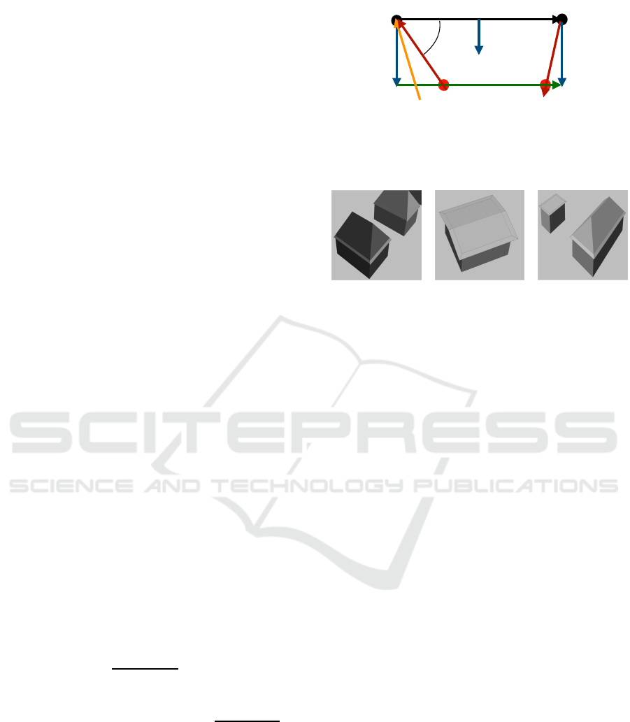
3.2 Connecting Roof Overhangs

In this section we discuss the scenario that overhangs

have to be attached to two roof ed ges that are incident

to the same vertex u in 3D, see examples in Figure

3. For simplicity, we describe the calculation for u

replaced by (0,0) so that the point u has to be added

to the re sulting 2D points, see Figure 4.

We shift the 2D roof edge indicated by ~a in Fig-

ure 4 belonging to a roof polygon with 3D normal ~n

by adding a 2D vector

that is o rthogo nal to ~a and

pointing outwards. Thus,

= s(~a.y,−~a.x) for some

s > 0. In the same way, we deal with the edg e indi-

cated by

b of the sec ond polygon and shift it with

orthogonal to

b and pointing ou tward.

Automatic Reconstruction of Roof Overhangs for 3D City Models

147

⃗

(0,0)

roof!with!normal!

⃗

ridge!line!between!roof!polygons

roof!with!normal!

⃗

Figure 4: Connecting two overhangs.

We obtain the intersection point P

of the bound-

ary of the overhang polyg on via

= (0,0) +

+ s

~a = (0, 0) +

+ s

b, (1)

i.e., by solving th e two corre sponding linear equations

with Cramer’s rule. If there is no unique intersec-

tion point (~a and

b are parallel), then the two over-

hang segments are treated separately at this vertex if

. We do not connect them. If the two vectors

are equal, we set s

= s

= 0 and can also use point

. If |P

| > |

| + |

| then the angle between ~a and

b is close to 180

◦

, and the segments are also treated

separately.

If~n

=~n

, the edges belong to the same roof facet.

In this case, the overhangs meet at the edge between

and (0,0). Otherwise, there exists an intersection

line between the two roof facets belonging to the two

roof edges. Then we also need to ﬁnd the intersection

with one of the two overhang edges. Using the

cross product, the direction of the ridge line can be

described with 2D vector

~r = ((~n

×~n

).x,(~n

×~n

).y). (2)

Then either

= s

~r = P

+ s

~a (3)

= s

~r = P

+ s

b. (4)

Both equations can be solved with Cramer ’s rule. If

a so lution does not exist, w e only co nsider the other

equation. If both solutions exist, we select one by

comparing s

and s

. If s

≥ 0 (or equivalently, s

≥

0), we compute P

with ( 4). Otherwise, P

is given by

(3) as shown in Figure 4.

To obtain the usual appearance of overhangs, we

add an additional point P

If P

results from (3), we project P

orthogonally

onto the line P

+ s

= P

+ s

= P

+ s

b. (5)

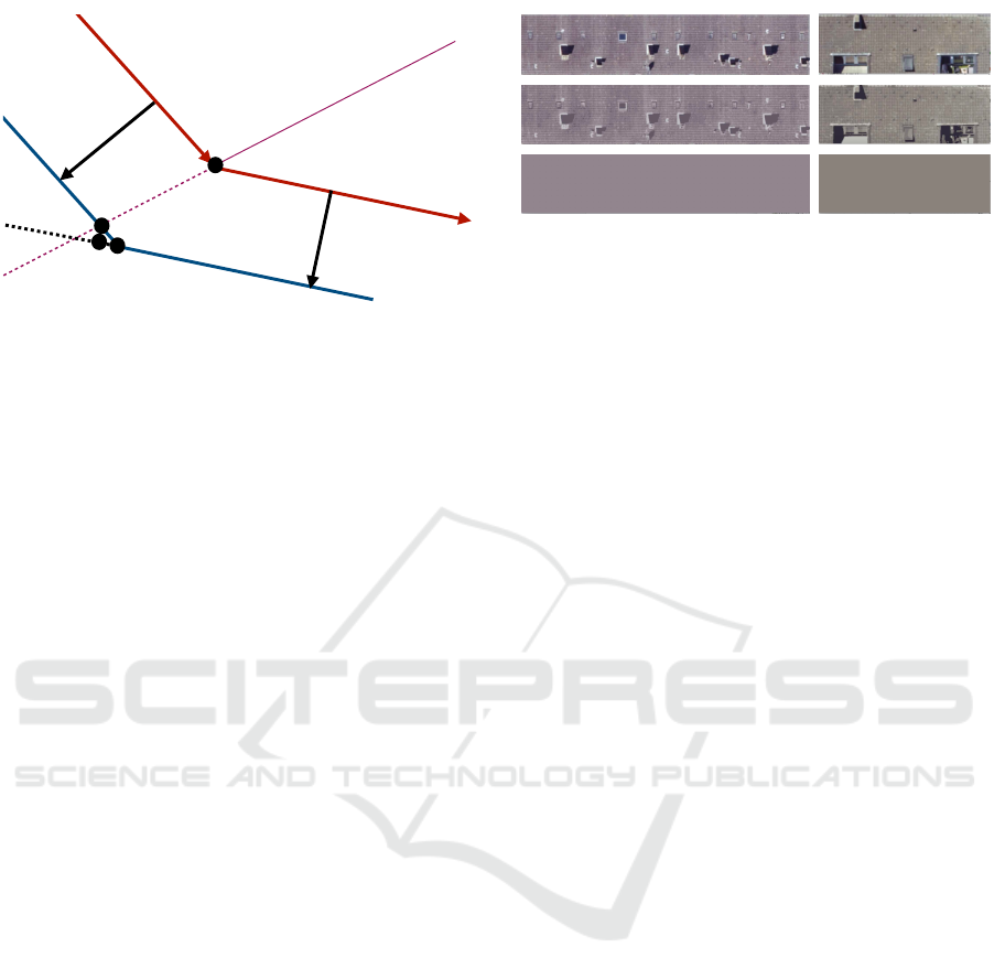
Figure 5: From top to bottom: original roof texture, texture

reduced to eight colors, and dominant color.

Then the points (0,0), P

, and P

are vertices of th e

left side of the overhang for edge

b, and the points P

and (0,0) are vertices of the right sid e of the overhang

for edg e ~a.

If P

is calculated with (4), we project P

onto the

line P

+ s~a:

= P

+ s

= P

+ s

~a. (6)

Then the points P

, P

and (0,0) are vertices of the

right side of the overhang for the edge ~a, and the

points (0 , 0) and P

are vertices of the left side of the

overhang for the edge

The orthogonal projection leading to P

could

cause an intersection with neighboring structures. We

replace

similar to ~n in Section 3.1 if nece s-

sary.

4 COLOR OF OVERHANGS

For textured city models, the overhang s may not be

fully visible in the textures provided. Therefore, we

do not equip overhangs with textures from the m odel,

but with the dominant color of the corresponding roof

facet. The do minant color is determined using the me-

dian cut a lgorithm (Heckbert, 1982). This algorithm

clusters color values iteratively by comparing values

of the c hannel with the largest range to their median.

Finally, the ch a nnel-wise arithm etic mean of all co l-

ors in a cluster is used to represent their replacement

color. Applied to a textur e image, the algorithm c a n

reduce the number of colors to very few, say eight.

Then the color with the largest number of pixels is

chosen, see Figures 5 and 6.

To obtain homogeneous looking roof planes, one

could also remove a ll roof textures and use th e

correspo nding colors instead. This also removes

perspective-distorted images of structures suc h as

dormers, which are not represented in LoD 2 mod els.

GRAPP 2023 - 18th International Conference on Computer Graphics Theory and Applications

148

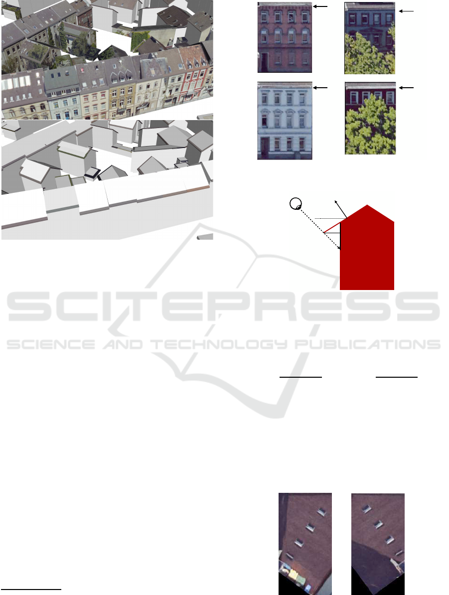
Figure 6: Overhangs painted with the main color of the cor-

responding roof facet.

5 SIZE OF OVERHANGS

5.1 Size Derived from Textures

For each ro of edge for which we have to construct an

overhang, we need to estimate the overhang size d,

as used in Sectio n 3.1, or the sizes |

| and |

|, as

used in Section 3.2. To th is end, we utilize textures

from CityGML models. Ma ny communities maintain

such texture d models. While the camera position and

parameters are p recisely kn own for oblique aerial im-

ages, the se data are not available for the textures. We

therefore assume – and this is not far-fetched – that fa-

cade images are generated from oblique aerial images

that are taken at a 45

◦

angle. Then roof overhangs

are visible in the top of facade textures

, see Figure 7.

Let h > 0 be the vertical extent of this texture region,

measured in meters. We derive the size of the over-

hang using h. If h > 2, i.e, the size exceeds typical

values, we assume that the size results fro m artifacts

and that the roof facet is not clearly visible in the fa-

cade image. Then we replace h by 2 for com puting

the box- plots bu t change the value to zero for recon-

structing overh angs. I f the roof edge belongs to a ﬂat

roof, then the size is d = h. Otherwise, let ~n be the

We textured a city model with oblique areal images

that were provided by the cadastral ofﬁce of the city of

Krefeld.

}

Figure 7: Overhangs with height h are visible in facade tex-

tures.

⃗

}

∘

}

Figure 8: Estimating the size d of an overhang with normal

~n from a texture in which the roof section has height h, see

(7).

normal of the corresponding roo f poly gon, then, see

Figure 8, tan(α) = d/(h − d) a nd

d = h ·

tan(α)

1 + tan(α)

, tan(α) =

~n.z

|(~n.x,~n.y)|

. (7)

To obtain h, we create an image based on texture co-

ordinates simulating a UV-mapping by applying ei-

ther an afﬁne transformation based on three polyg on

vertices or by a perspective transform based on four

polygon vertices with the OpenCV library. Then we

shift, rotate, and cut off the image su ch that the roof

edge corresponds with the top boundary of the ima ge,

see facades in Figur e 7 and 9.

Figure 9: Rotated wall texture: The upper boundary of each

image coincides with the roof edge to be examined.

Automatic Reconstruction of Roof Overhangs for 3D City Models

149

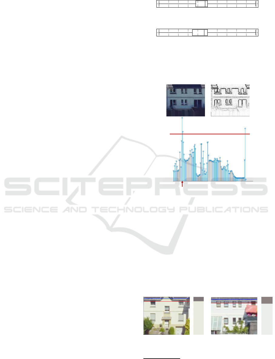
Then, h can be determined using image processing

methods. We compare two approache s, one based on

an edge image and one based on homogeneous color

regions.

After creating an edge image, the edge pixels per

line are summed to get a histogram function. Then,

the function is normalized so that the smallest value

is 0 and the largest value is on e. We seek for the

ﬁrst value that exceeds the experimentally determined

threshold of 0.75, see Figure 11. Considering the im-

age resolution, the corr e sponding lin e index deﬁnes

h. Since it has been found that dominant edge s often

appear at the bottom of facades, we restrict the com-

putation to the upper half of the texture.

The second approach is based on color regions.

With the media n cut algorithm, cf. Section 4, we de-

termine both the dominan t color of the facade and the

dominant color of the cor respond ing roof facet. Based

on the transformed texture image with n rows, a his-

togram function is com puted. This fu nction maps th e

line index to the number of those pixels in the image

line f or which the l

-distance o f the R-G-B color to

the roof color is smaller than a quarter of the distance

to the facade color. Then the histogram function is

scaled so that its minimum is z e ro and its ma ximum

is one. We denote this function by f . In an ideal

world, where the pixels can be uniquely assigned to

either the roof or the facade such that the correspond-

ing regions are divided horizontally b y a line, f is a

function of type g

with

(k) :=



1 : k ∈ {0, 1,...,l}

0 : k ∈ {l + 1,... , n − 1}.

(8)

Therefore, we compute th e smallest line index l for

which

∑

⌊n/2⌋−1

k=0

( f (k) − g

(k))

is minimal. Again, we

focus on the upper ha lf of the image and obtain h fro m

this smallest line index as w e ll by considering the im-

age resolution. Figure 12 dem onstrates the concept

but also shows that shadows of overhangs c an extend

the roof area.

For the automatic reconstruction o f overhangs, the

minimum size of bo th appro aches can be used. Roof

and wall textures can co me from different aerial or

oblique aerial images with different cameras. There-

fore, it is not surprising that both approaches lead

to differences tha t are shown in Figure 10 for the

square kilometers speciﬁed by zon e 32U UTM in-

terval [330,0 00; 331,000] × [5,687 , 000; 5,688,000]

(8,261 roof edges with available roo f and facade tex-

tures) and the next interval [330 , 000; 331,0 00] ×

[5,688,000; 5, 689,000] (7,733 roof edges). These

square kilometers are used in other ﬁgures, too.

-2.0 -1.6 -1.2 -0.8 -0.4 0 0.4 0.8 1.2 1.6 2.0 m

arithmetic mean: -0.306 m

-2.0 -1.6 -1.2 -0.8 -0.4 0 0.4 0.8 1.2 1.6 2.0 m

arithmetic mean: -0.384 m

Figure 10: Differences between overhang sizes estimated

based on dominant colors and overhang sizes estimated with

an edge image; the box plots belong to different square kilo-

meters.

.75

Figure 11: Detection of roof regions with edge histograms.

5.2 Size Derived from a Point Cloud

Figures 14 an d 15 demon stra te that overhangs are in-

deed visible even in sp arse airborne laser scanning

point clou d data

. When such a point cloud is avail-

able, we also use it to compu te sizes of overhangs. To

this end, we organize the point clouds in a q uad-tree

for faster access. For each relevant roof edge, we co n-

sider a rectangular ar ea in the x-y ground plane. One

side of this rectangle is given by the middle part of the

roof e dge (with half the leng th o f the edge to avoid

interference with other structures at the corners). The

rectangle extends two meters beyond the roof facet.

Figure 12: The blue lines separate the roof and facade based

on an edge image, the red lines separate the dominant colors

of the roof and facade.

Available from Geobasis NRW, https://

www.bezreg-koeln.nrw.de/brk_internet/geobasis/

hoehenmodelle/3d-messdaten/index.html

GRAPP 2023 - 18th International Conference on Computer Graphics Theory and Applications

150

-2.0 -1.6 -1.2 -0.8 -0.4 0 0.4 0.8 1.2 1.6 2.0 m

arithmetic mean: -0.349 m

-2.0 -1.6 -1.2 -0.8 -0.4 0 0.4 0.8 1.2 1.6 2.0 m

arithmetic mean: -0.187 m

Figure 13: Quality of overhang sizes estimated from sparse

airborne laser scanning point clouds: The box plots show

the distribution of differences between σ and γ (see Section

5.2) for the same two square kilometers as in Figure 10.

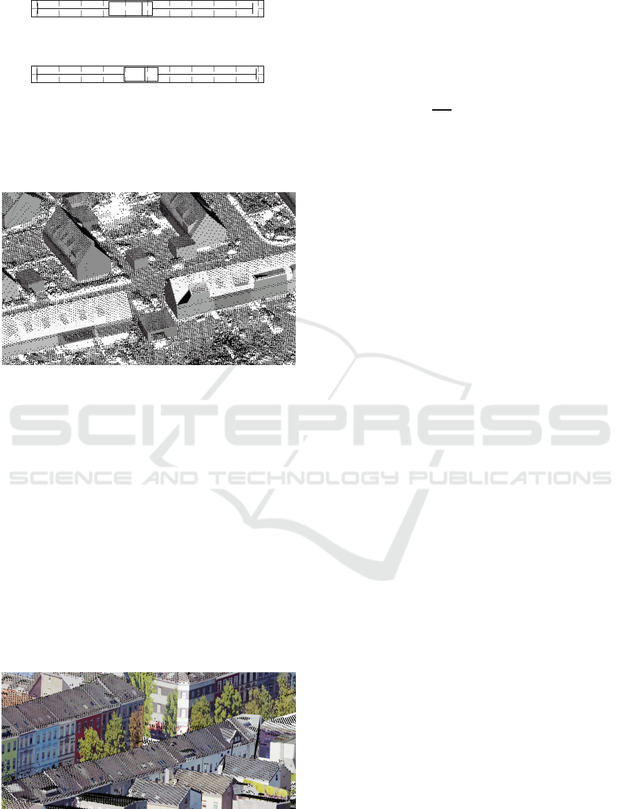
Figure 14: Matching of an airborne laser scanning point

cloud with an LoD 2 city model: Visible black points of the

cloud are not occluded by the model.

Larger overhangs occur only very rarely and pose the

risk of overlapping with other buildings. Then all

laser scanning poin ts within this rectang le are deter-

mined and their distance to the boundless roof plane

belonging to the edge is calcu late d by using the Hesse

normal form with the given plane normal. If a dis-

tance is below one meter, the point is considered as

a plane in lier. Let γ be the largest distance of all in-

liers to the edge under consideration. If there are no

inliers, γ is set to zero. We have an outlier point, if its

distance to the plane exceeds one meter. This thresh-

old is chosen to ignore no ise and because almo st all

facades are higher than two me te rs. Outliers are ig-

nored if they are above the plane. This is necessary

to avoid false outliers, e.g., due to dormers that are

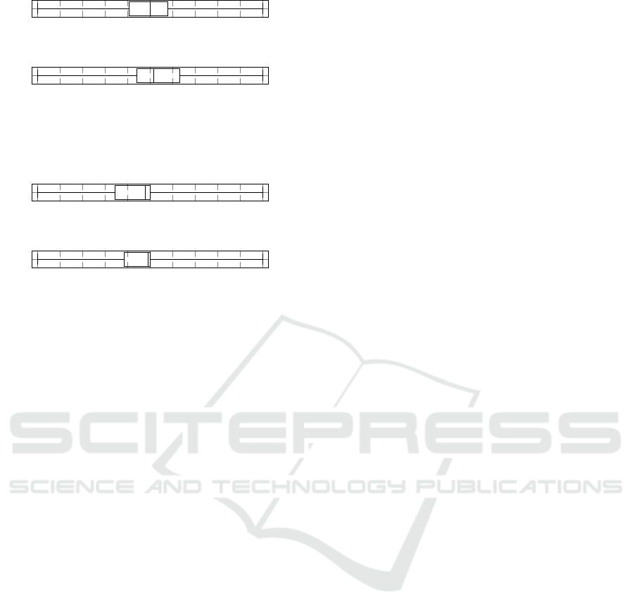
Figure 15: Roof regions shown in facade t extures of an LoD

2 city model indeed correlate with point cloud points be-

longing to roof overhangs.

missing in the given building model. Outliers below

the p la ne indicate the end of the roof facet. Let σ

be the shortest distance of all outliers to the edge. If

there are no such ou tliers, σ is set to th e maximu m

overhang size of 2 m. Finally, we estimate the size d

of the overhang :

d :=



γ+σ

: outliers exist

γ : otherwise.

(9)

Figure 13 shows differences between γ and σ for

sparse airborne laser scanning point clouds in c on-

junction with roof facets of a city model com-

puted on these data and on cadastral footprints using

RANSAC. One would expect σ > γ with the differ-

ence being small. Inliers should be near the roof edge,

and outliers should be farther away. However, the

LoD 2 mode ls have simpliﬁed roof topologies. For

example, a roof facet may be separated by a dormer so

that ther e is no overhang in front of the dormer. But

the d ormer may be ab sent from the model, leading

to outliers close to the roof edge under consideratio n.

Also, vegetation leads to false inliers.

6 RESULTS

Since we are not aware of any ground truth, we com-

pare sizes of overhangs obtained from facade textures

(included in a CityGML model and previously com-

puted from o blique areal images with a pixel size

of about 0.1 m × 0.1 m) on the one hand and from

airborne laser scanning point clouds (provided by

Geobasis NRW with a resolution between 5 and 10

points per square meter ) on the other hand. The dif-

ferences between these size estimates are shown in

Figures 16 and 17. Compared to the size of the over-

hangs, the d ifferences between the size estimates are

substantial. However, apart from the implicit inac-

curacies in the estimatio n methods, the reasons for

this also lie in the data. Roof planes in 3D c ity mod-

els usually simplify real roof structures. In reality,

walls have a certain thickness that they do not have in

the model. Cadastral footprints do not exactly match

oblique aerial imag e data. These inaccuracies result

in texture shifts. Textures can show objects or other

buildings that occlud e the wall in question. We also

use a point cloud from airborne laser scanning, whose

relative accuracy within the cloud is very good, but

the entir e cloud may be slightly shifte d compared to

cadastral data. The point cloud is sparse, so small

structures such as overhangs are barely represented.

Automatic Reconstruction of Roof Overhangs for 3D City Models

151

-2.0 -1.6 -1.2 -0.8 -0.4 0 0.4 0.8 1.2 1.6 2.0 m

arithmetic mean: 0.006 m

-2.0 -1.6 -1.2 -0.8 -0.4 0 0.4 0.8 1.2 1.6 2.0 m

arithmetic mean: 0.148 m

Figure 16: Size estimates based on texture edges minus esti-

mates from aerial laser scanning point clouds for two square

kilometers.

-2.0 -1.6 -1.2 -0.8 -0.4 0 0.4 0.8 1.2 1.6 2.0 m

arithmetic mean: -0.302 m

-2.0 -1.6 -1.2 -0.8 -0.4 0 0.4 0.8 1.2 1.6 2.0 m

arithmetic mean: -0.238 m

Figure 17: Size estimates from texture colors minus esti-

mates from aerial laser scanning point clouds for two square

kilometers.

7 CONCLUSIONS

With the developed tool, roof overhangs can be added

to existing CityGML models with or without usin g

additional data, giving the models a much more real-

istic appear a nce. The tested heuristics for estimating

the size of the overhangs work in principle, but with

the poor-resolution im age and point cloud data avail-

able to us, the estimates a re comparatively inaccurate.

Better quality can be expected, for exam ple, when us-

ing higher resolution point clouds, but they are not

available throughout a widespre ad area.

Flat roofs often do not have overhangs but a small

elevated frame along their perimeter. Such frames can

be added to city models in a similar way as overhangs,

by extending edges into direction −~n, see Sectio n 3.1,

and without considering ridge lines, cf. Section 3.2.

Future work may also explore estimating the size of

roof overhangs using machine learning.

ACKNOWLEDGMENTS

The authors are grateful to Udo Hannok from the

cadastral ofﬁce of the City of Krefeld for providing

oblique aerial image s. T he authors are also grateful

for valuable comments by the anonymous reviewers.

REFERENCES

Biljecki, F., Stoter, J., Ledoux, H., Zlatanova, S., and Çöl-

tekin, A. (2015). Applications of 3D city models:

State of the art review. ISPRS International Journal

of Geo-Information, 4:2842–2889.

Chen, Q., Wang, L., Waslander, S. L., and Liu, X. ( 2020).

An end-to-end shape modeling framework for vector-

ized building outline generation from aerial images.

ISPRS Journal of Photogrammetry and Remote Sens-

ing, 170:114–126.

Chen, Y., Cheng, L., Li, M., Wang, J., Tong, L., and Yang,

K. (2014). Multiscale grid method for detection and

reconstruction of building roofs from airborne LiDAR

data. IEEE J. Sel. Topics Appl. Earth Observ. Remote

Sens., 7(10):4081–4094.

Cheng, D., Liao, R., Fidler, S., and Urtasun, R. (2019).

DAR-Net: Deep active ray network for building seg-

mentation. In Proc. IEEE/CVF Conference on Com-

puter Vision and Pattern Recognition (CVPR), pages

7423–7431.

Dahlke, D., Linkiewicz, M., and Meissner, H. (2015). True

3D building r econstruction: Façade, roof and over-

hang modelling from oblique and vertical aerial im-

agery. International Journal of Image and Data Fu-

sion, 6(4):314–329.

Frommholz, D., Linkiewicz, M., Meißner, H., and Dahlke,

D. (2017). Reconstructing buildings with disconti-

nuities and roof overhangs from oblique aerial im-

agery. International Archives of Photogrammetry and

Remote Sensing, XLII -1 (W1):465–471.

Goebbels, S. and Pohle-Fröhlich, R. ( 2020). RANSAC for

aligned planes with application to roof plane detection

in point cl ouds. In Proc. GRAPP, pages 193–200.

Gröger, G., Kolbe, T. H., Nagel, C., and Häfele, K. H.

(2012). OpenGIS City Geography Markup Language

(CityGML) Encoding Standard. Version 2.0.0. Open

Geospatial Consortium.

Heckbert, P. (1982). Color i mage quantization for frame

buffer display. Computer Graphics, 16(3).

Kutzner, T., Chaturvedi, K., and Kolbe, T. H. (2020).

CITYGML 3.0: New functions open up new appli-

cations. PFG, 88:43–61.

Malhotra, A., Raming, S., Frisch, J. , and van Treeck, C.

(2021). Open-source tool for transforming CityGML

levels of detail. Energies, 14(24).

Oestereich, M. (2014). Das 3D-Gebäudemodell im Level

of Detail 2 des Landes NRW. Nachrichten aus dem

öffentlichen Vermessungswesen Nordrhein-Westfalen,

47(1):7–13.

Wang, R., Peethambaran, J., and Chen, D. (2018). LI DAR

point clouds to 3-D urban models: A review. IEEE

Journal of Selected Topics in Applied Earth Observa-

tion and Remote Sensing, 11(2):606–627.

Yan, J., Jiang, W., and Shan, J. (2012). Quality analysis on

RANSAC-based roof facets extraction from airborne

LIDAR data. International Archives of Photogramme-

try and Remote Sensing, XXXIX(B3):367–372.

GRAPP 2023 - 18th International Conference on Computer Graphics Theory and Applications

152