Integrated Production and Energy Supply Planning on an Industrial Site

by Mixed-Integer Linear Programming

Ruiwen Liao and C

eline Gicquel

Laboratoire Interdisciplinaire des Sciences du Num

erique, Universit

e Paris Saclay, France

Keywords:

Production Planning, Lot-Sizing, Renewable Energy, Energy Supply, Mixed-Integer Linear Programming.

Abstract:

Industrial production sites are nowadays faced with two major concerns: the need to reduce the environmental

impact of their processes and the economic difﬁculties caused by the rising energy prices. Both challenges may

be partially tackled by powering industrial processes with electricity generated on-site from renewable sources.

However, the volatility of the electricity prices and the intermittence of the locally generated renewable energy

sources result in the need to solve an integrated industrial production and energy supply planning problem.

This work investigates a single-machine multi-product lot-sizing problem for an industrial process powered by

both grid electricity and on-site renewable energy. We propose a new extension of the Proportional Lot-sizing

and Scheduling Problem relying on a two-level structure for time discretization. The ﬁrst level is related to

the product demand satisfaction, the second one is used for both production and energy supply planning. The

proposed extension is compared to a previously published extension of the General Lot-sizing and Scheduling

Problem dealing with a similar problem. Our preliminary numerical results show that in most cases, our model

provides a production plan of the same cost, but with a signiﬁcantly reduced computational effort.

1 INTRODUCTION

Industrial companies are increasingly under pressure

to mitigate the CO2 and pollution emissions linked

to the manufacturing of industrial products. They are

also confronted with a sharp rise of the price of con-

ventional energy sources (gas, grid electricity...) so

that the availability and affordability of energy is be-

coming a critical parameter in manufacturing. One

way to deal with these two challenges consists in pow-

ering industrial processes with electricity generated

on-site from renewable sources.

In an industrial production plant, the energy man-

agement system is usually limited to two elements:

the energy bought from an outside supplier on the na-

tional market and the energy consumed by the manu-

facturing processes. As conversion devices (e.g. wind

turbines, photovoltaic panels) able to produce elec-

tric power from renewable energy sources are becom-

ing less expensive, it is now possible for an industrial

plant to build its own environmental friendly energy

system and to use this ’green’ electricity to power its

processes. For example, more than 30000 solar panels

have been installed on the rooftop of Bentley’s factory

in Crewe as well as on the roof of its carport, which

provide up to two third of the factory’s energy demand

with a power generation capacity of 7.7kW. In Cal-

ifornia, the brewery factory Anheuser-Busch’s Bud-

weiser installed 6500 solar panels as well as wind tur-

bines, which provide 30% of the factory’s electricity

use. Batteries may also be installed to store electric-

ity. However, the intermittence of renewable energy

sources (wind, sun...) makes it impossible to fully re-

place gas or grid electricity by on-site generated elec-

tricity to power an industrial process: both types of

energy should thus be used in combination. More-

over, the time-of-use pricing scheme widely used by

electricity providers means that it is necessary to ac-

curately track the timing and quantity of grid electric-

ity bought from these providers. In this circumstance,

making sure that energy supply and consumption are

balanced at all time is challenging. Thus, an inte-

grated energy supply and industrial production plan-

ning problem needs to be solved.

With all these challenges mentioned above,

energy-efﬁcient production planning has attracted

great research attention in the last decades (Terbrack

et al., 2021; Gao et al., 2020). Some works con-

sider that all the needed energy comes from electricity

bought from the main electric grid at a time-varying

price and introduce energy consumption costs in the

objective function of the production planning model:

Liao, R. and Gicquel, C.

Integrated Production and Energy Supply Planning on an Industrial Site by Mixed-Integer Linear Programming.

DOI: 10.5220/0011602900003396

In Proceedings of the 12th International Conference on Operations Research and Enterprise Systems (ICORES 2023), pages 119-126

ISBN: 978-989-758-627-9; ISSN: 2184-4372

 2023 by SCITEPRESS – Science and Technology Publications, Lda. Under CC license (CC BY-NC-ND 4.0)

119

see e.g. (Johannes et al., 2019). Other works study

the case where energy can be obtained from both the

main electric grid and a non-adjustable on-site elec-

tricity generation system based on renewable energy

sources. Most of these studies focus on the short-

term scheduling of a job shop (Golp

ıra et al., 2018)

or a ﬂow shop (Biel et al., 2018; Wang et al., 2020).

However, lot-sizing in the presence of intermittent re-

newable energy sources has been rarely studied in the

literature. (Rodoplu et al., 2019) addressed a single-

item multi-machine lot-sizing problem. Chance con-

straints were introduced to deal with the ﬂuctuation of

renewable energy sources. A lot-sizing and schedul-

ing problem was investigated in (Wichmann et al.,

2019), with consideration of renewable energy re-

sources and energy storage system.

The present work focuses on a short-term produc-

tion planning problem, namely a multi-item single-

machine lot-sizing problem, and seeks to integrate

the energy supply planning into the problem mod-

eling. Basically, a lot-sizing problem is a produc-

tion planning problem in which we seek to ﬁnd the

optimal trade-off between the startup and inventory

holding costs. Startup costs are ﬁxed costs occur-

ring every time the machine’s status changes in or-

der to process of a new type of product, while in-

ventory holding costs represent the costs of keeping

ﬁnished products in inventory between the time they

are produced and the time they are used to satisfy the

customers’ demand. In our case, the energy supply

system comprises three main elements: on-site power

generation devices producing a time-varying amount

of green electricity from renewable energy sources, an

on-site energy storage system and the main electric

grid with which electricity may be traded at a time-

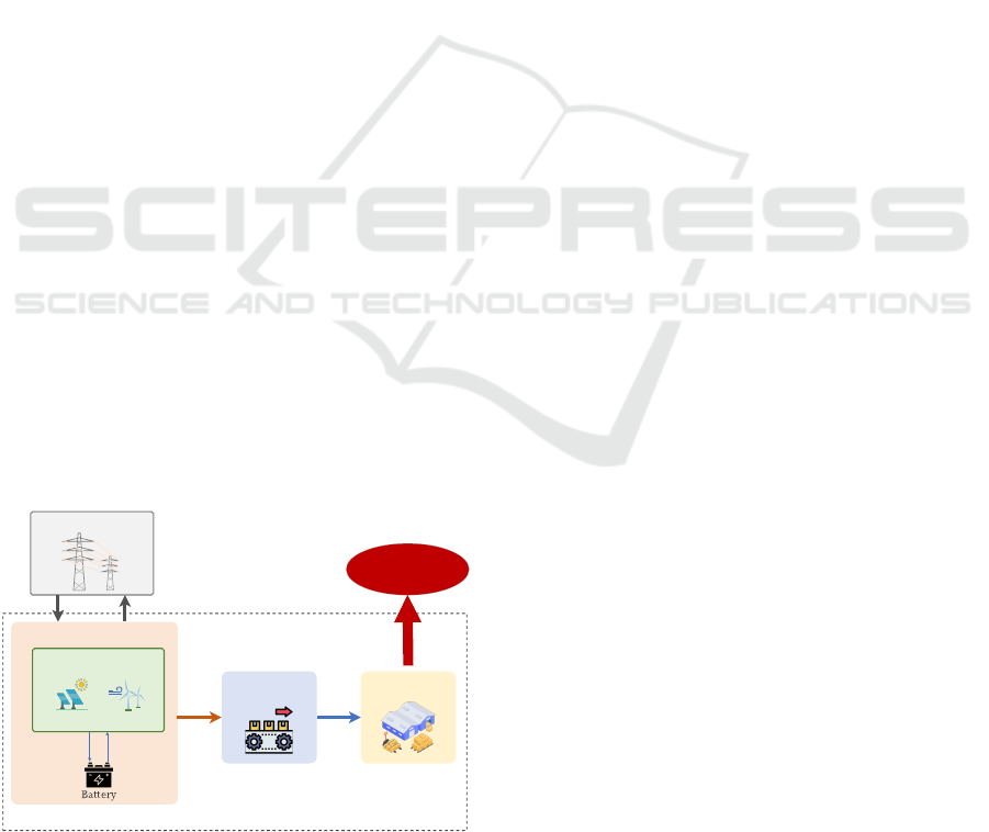
varying price. See Figure 1 for a graphical represen-

tation of the studied integrated energy supply and in-

dustrial production system.

Inventory

Power generation devices using

renewable energy sources

Wind turbine

PV panel

Main grid

Energy system

External

demands

Integrated system

Production

system

Figure 1: Integrated energy supply and industrial produc-

tion system.

One modelling difﬁculty here comes from the fact

that the time discretization needed to manage prod-

uct demand satisfaction, production planning and en-

ergy supply may signiﬁcantly differ. Indeed, follow-

ing the terminology introduced by (Copil et al., 2017),

we have to handle two exogenous time structures, i.e.

two sets of points in time at which externally given

events, that are deﬁned by the data of the model, are

considered. The ﬁrst time structure is imposed by the

timing of the external demand and usually uses rather

large time buckets (typically days or weeks). The sec-

ond one is imposed by the discrete time grid used to

track the availability of the on-site generated electric-

ity and the varying price of grid electricity. This time

grid usually uses much smaller time buckets (typi-

cally hours or 10-minutes intervals). In between these

two exogenous time structures, to plan production, we

have to handle a third endogenous time structure rep-

resenting the points in time at which internal events

are captured by decision variables.

As mentioned above, the problem of determining

optimal production lot sizes under intermittent renew-

able energy has been scarcely studied in the litera-

ture. A noticeable exception can be found in (Wich-

mann et al., 2019). This paper namely investigates

an integrated industrial production and energy sup-

ply planning problem for a manufacturing site pow-

ered by a decentralized power system using renew-

able energy sources. Their problem modeling relies

on a three-level time structure: a coarse time dis-

cretization to track the customers’ demands, a ﬁne

energy-oriented time discretization to track the varia-

tions in the energy price and availability, and another

ﬂexible production-oriented ﬁne discretization to de-

termine the production plan. The resulting model can

be seen as an extension of the General Lot-sizing and

Scheduling Problem (GLSP) introduced by (Fleis-

chmann and Meyr, 1997) and takes the form of a

large-size mixed-integer linear program (MILP) for-

mulation involving many big-M constraints. Conse-

quently, numerical difﬁculties arise when trying to

solve medium-size instances of the problem with a

mathematical programming solver.

This is why we propose in this paper a new model

for the integrated energy supply and industrial pro-

duction planning problem. This model relies on a

two-level time structure. This one consists in a coarse

time discretization to track the demand satisfaction

and in a single ﬁne time discretization based on the

exogenous time structure imposed by the energy-

related input data. This ﬁne time discretization is used

both to track the variations in the energy price and

availability and to plan the industrial production. The

use of a ﬁxed time grid involving short planning pe-

ICORES 2023 - 12th International Conference on Operations Research and Enterprise Systems

120

riods to determine the production lot sizes leads to

the formulation of a ’small bucket’ lot-sizing prob-

lem, i.e. to the formulation of a lot-sizing problem

in which there are some restrictions on the number

of item types that may be produced in each planning

period. More precisely, we consider here the Pro-

portional Lot-sizing and Scheduling Problem (PLSP)

in which at most two different types of product may

be produced in each period: see (Drexl and Haase,

1995). The main advantage of the proposed modeling

approach is that it leads to an MILP formulation much

smaller that the one obtained with the model proposed

in (Wichmann et al., 2019).

Our contributions are thus twofold. First, we pro-

pose a new extension of the PLSP in order to simulta-

neously plan the industrial production and the energy

supply in a manufacturing plant powered, at least par-

tially, by a decentralised energy system using renew-

able energy sources. Second, we carry out numerical

experiments to compare the proposed model with the

GLSP-based model previously published by (Wich-

mann et al., 2019). Our numerical results show that

in most cases, our model provides a production plan

of the same cost than the one provided by the model

introduced by (Wichmann et al., 2019) but with a sig-

niﬁcantly reduced computational effort.

The paper is organized as follows. Section 2 pro-

vides a detailed description of the optimization prob-

lem under study. Section 3 presents the proposed

PLSP-based model based on a two-level time struc-

ture. Section 4 discusses the results of the compu-

tational experiments conducted on medium-size ran-

domly generated instances. Conclusion and research

perspectives are given in Section 5.

2 PROBLEM DESCRIPTION

We seek to plan production over a ﬁnite horizon in an

industrial plant producing J types of item. The set of

items is denoted as J = {1, 2,..., J}. A ﬁrst exoge-

nously imposed time grid is introduced to track the

points in time at which the external customers’ de-

mand occurs. The planning horizon is thus divided

into a set T = {1,2,. ..,T } of macroperiods of ﬁxed

length l: the end of each macroperiod corresponds to

a point in time at which demand may occur. Let d

j,t

denote the demand for item j to be satisﬁed at the end

of macroperiod t. Backlogging is not allowed, i.e., all

the demand should be satisﬁed on time. At the end

of each macroperiod, the ﬁnished products remaining

after the demand has been satisﬁed are held in inven-

tory in the warehouse for later use. Each unit of item

j held in inventory between two macroperiods incurs

a unit cost h

. The initial inventory of item j is given

j,0

We assume that the production process comprises

a single production resource. This resource may be in

three distinct kinds of states: idle, setup for a given

item, and manufacturing a given item. The resource

is idle when it is turned on but not ready for produc-

tion. It may also be setup for a speciﬁc item: in this

case, it is ready to produce this type of item but is not

producing it. Finally, the resource is in a item-related

manufacturing state when it is actually producing this

speciﬁc type of item: this is however possible only

if the resource is already set up for this type of item.

Let k

be the amount of time needed to produce one

unit of item j on the resource. A startup is the action

of changing the machine status to prepare it to pro-

duce a new type of item. A startup for item j thus

occurs whenever the state of the resource is switched

from any other idle, setup or manufacturing state to

the setup state corresponding to this item. Let f

the ﬁxed startup cost to be paid each time a startup for

item j happens. All startup times are assumed to be

negligible.

Energy is consumed by startups and manufactur-

ing. The amount of energy consumed during a startup,

denoted by e

, depends on the product that the ma-

chine will be setup for. The energy consumed during

manufacturing is proportional to the number of items

produced. Let e

denote the energy needed to produce

one unit of item j. We assume that no energy is con-

sumed when the machine is idle or when it is setup

for a given product but not producing.

The energy is supplied either from the main grid

or from the on-site renewable energy conversion de-

vices. The necessity to track the time variations of

the main grid energy price and of the amount of en-

ergy generated by the on-site power system leads us

to consider a second exogenously imposed time grid.

This one is based on planning periods sufﬁciently

short to assume that the energy price and the green

energy power generation are constant during a pe-

riod. Each macroperiod t = 1, ...,T of length l is

thus split into n energy-oriented microperiods of ﬁxed

length l

such that l = nl

. Let R = {1, ...,nT } be

the set of all energy-oriented microperiods and R

{(t −1)n + 1, ...,tn} be the set of energy-oriented mi-

croperiods belonging to macroperiod t. We denote

by e

(resp e

) the purchasing (resp. selling) price

of the energy traded with the main grid during mi-

croperiod r. Since the voltage of electricity used for

long-distance transmission by the grid operator is not

the same as the one used in the manufacturing plant,

a grid transformer is needed to adapt the electricity to

production use. This causes energy losses mostly due

Integrated Production and Energy Supply Planning on an Industrial Site by Mixed-Integer Linear Programming

121

to the electrical current ﬂowing in the coils and the

magnetic ﬁeld alternating. We denote by η

the efﬁ-

ciency of the grid transformer. The amount of green

electricity generated on-site by the local energy sys-

tem during micro-period r is denoted by p

Finally, the energy storage system consists of a

battery which can store the residual electricity gener-

ated by the on-site power conversion devices and the

energy bought from the main grid. Let c

be the max-

imum amount of energy that can be stored in this sys-

tem. The amount of energy which can be charged into

(resp. discharged from) the battery during an energy-

oriented microperiod is denoted by m

(resp. m

Battery charging/discharging incurs some energy loss

due to the internal resistance: let η

/η

be the charg-

ing/discharging efﬁciency of the battery.

The optimization problem under study here con-

sists in building an integrated energy supply and pro-

duction plan. This plan should simultaneously deter-

mine when and how many ﬁnished products to pro-

duce and when and how much energy to trade with

the grid and to charge into/discharge from the battery.

This plan should ensure that the demand for the ﬁn-

ished products is satisﬁed at all time and that there

is always enough energy to supply the manufacturing

process while minimizing the total production and en-

ergy procurement costs.

3 PLSP-BASED MODEL

As will be shown by the numerical experiments to be

provided in Section 4, using the GLSP-based model

previously published by (Wichmann et al., 2019) to

build a production and energy supply plan is pos-

sible only for small instances. Signiﬁcant compu-

tational difﬁculties are encountered when trying to

solve medium to large size instances. These difﬁcul-

ties mainly come from the sharp increase in the size of

the MILP formulation with the number of items and

horizon length. In order to overcome this, we propose

a new PLSP-based model for the problem relying on

the use of small buckets to plan production.

3.1 Model Description

The main idea underlying the proposed PLSP-based

model consists in aligning the production-related time

discretization on the energy-related time discretiza-

tion and to deﬁne the production plan using the ex-

ogenously deﬁned energy-oriented microperiods. The

use of a ﬁxed time grid involving short planning pe-

riods to determine the production lot sizes leads to

the formulation of a ’small bucket’ lot-sizing prob-

lem, i.e. to the formulation of a lot-sizing problem

in which there are some restrictions on the number

of item types that may be produced in each planning

period. More precisely, we consider here the Propor-

tional Lot-sizing and Scheduling Problem (PLSP) in

which at most two different types of item may be pro-

duced in each energy-oriented microperiod. The use

of a ﬁxed time grid (rather than a ﬂexible one as done

in the GLSP) to plan production signiﬁcantly sim-

pliﬁes the mathematical formulation of the problem

as it eliminates the need to manage the intersections

between energy-oriented and production-oriented mi-

croperiods, which requires a large number of addi-

tional binary variables and big-M type constraints.

In order to formulate the problem as an MILP, we

introduce the following decision variables:

• I

j,t

: amount of item j held in inventory at the end

of macroperiod t,

• Y

j,r

: setup state of the resource at the end energy-

oriented micro-period r; Y

j,r

= 1 if the resource is

setup to produce item j at the end of r, Y

j,r

= 0

otherwise.

• X

j,r

: startup indicator. X

j,r

= 1 if there is a startup

for item j during r, X

j,r

= 0 otherwise,

• Q

j,r

: quantity of item j produced in energy-

oriented microperiod r.

• P

: amount of energy charged into / dis-

charged from the battery during energy-oriented

microperiod r,

• P

: state of charge of the battery at the end of

energy-oriented microperiod r,

• P

: amount of electricity purchased from /

sold to the main grid during energy-oriented mi-

croperiod r.

3.2 MILP Formulation

Objective Function. The objective function aims at

minimizing the total startup, inventory holding and

energy costs over the planning horizon.

min

∑

r=1

∑

j=1

· X

j,r

∑

t=1

∑

j=1

· I

j,t

∑

r=1

· P

− e

· P

(1)

Production-Oriented Constraints. We ﬁrst focus

on the set of production-oriented constraints. These

constraints aim at building a feasible production plan.

j,t

= I

j,t−1

∑

r∈R

j,r

− d

j,t

, ∀ j ∈ J ,t ∈ T . (2)

ICORES 2023 - 12th International Conference on Operations Research and Enterprise Systems

122

j,r

6 l(Y

j,r−1

j,r

), ∀ j ∈ J , r ∈ R . (3)

∑

j=1

j,r

6 l, ∀r ∈ R . (4)

∑

j=1

j,r

6 1, ∀r ∈ R . (5)

j,r

> Y

j,r

−Y

j,r−1

, ∀ j ∈ J , r ∈ R . (6)

j,r

j,r−1

6 1, ∀ j ∈ J ,r ∈ R . (7)

j,0

= 0, ∀ j ∈ J . (8)

j,0

, ∀ j ∈ J . (9)

j,T

> I

j,0

, ∀ j ∈ J . (10)

Constraints (2)-(6) deﬁne the production plan ac-

cording to the assumptions used in the PLSP. Con-

straints (2) are the inventory balance equations. In-

equalities (3) ensure that item j can be produced in

microperiod r only if the machine is set up for j at

the beginning or/and at the end of the period. Con-

straints (4) make sure that the total capacity consumed

by the production taking place during each micrope-

riod r stays below the capacity available in r. Equa-

tions (5) guarantee that the machine is set up for at

most one item at the end of each microperiod. To-

gether with Constraints (3), they ensure that at most

two items may be produced during a microperiod r.

The relationship between startup and setup decision

variables is described by (6): if the machine is setup

for item j at the end of r but was not setup for j at

the end of the r −1, a startup for j must occur during

r. (7) are basic valid inequalities that may be used to

strengthen the MILP formulation: see (Belvaux and

Wolsey, 2001). They indicate that if the machine was

already set up for j at the end of r − 1, then there is

no need to carry out a start up for item j during r. In-

versely, if a startup for product j occurs in r, it means

the machine was not set up for this product in r − 1.

Constraints (8)-(10) deﬁne the initial and ﬁnal condi-

tions.

Energy-Oriented Constraints. We now focus on

the set of energy-oriented constraints aiming at build-

ing a feasible energy supply plan in each energy-

oriented micro-period.

= η

·P

+ p

+η

·P

, ∀r ∈ R .

(11)

= P

r−1

+ P

− P

, ∀r ∈ R . (12)

0 6 P

6 c

, ∀r ∈ R . (13)

6 m

, ∀r ∈ R . (14)

6 m

, ∀r ∈ R . (15)

Equalities (11) ensure that the energy supply and

demand is balanced within each microperiod. The

energy demand consists in the energy consumed by

the manufacturing process P

, the energy sold to the

main grid P

/η

and the energy charged into the

battery P

/η

. Note how, since part of the energy

is lost within the grid transformer, the amount of en-

ergy needed to sell P

to the main grid is given

by P

/η

. Similarly, the actual energy needed to

charge P

into the battery is computed by P

/η

due

to the losses during the battery charging process. The

energy supply consists in the energy purchased from

the grid η

· P

, the energy generated from the re-

newable resources p

and the energy discharged from

the battery η

·P

. Note that, when we buy P

from

the main grid, only η

· P

energy is really available

for the plant. The same applies for the energy dis-

charging process. The energy balance in the battery

is deﬁned by Equations (12). The amount of energy

stored in the battery at the end of microperiod r is

equal to the amount stored at the beginning of r plus

the amount charged into the battery during r minus the

amount discharged from s. Constraints (13) impose

that the amount of energy stored in the battery does

not exceed its capacity. Inequalities (14) and (15) are

the battery maximum charging and discharging rate

constraints.

Coupling Constraints. The ﬁnal set of constraints

links together the decision variables related to produc-

tion and the one related to energy supply.

∑

j=1

· X

j,r

∑

j=1

· Q

j,r

, ∀r ∈ R . (16)

Equations (16) guarantee that the energy con-

sumption by the factory equals to the sum of the en-

ergy consumed for the startups and for the production

on the machine.

Domain Deﬁnition Constraints. Finally, the deﬁ-

nition domain of the decision variables are given by

Constraints (17)- (19).

j,r

∈ {0, 1},∀ j ∈ J ,r ∈ R , (17)

Integrated Production and Energy Supply Planning on an Industrial Site by Mixed-Integer Linear Programming

123

j,t

j,r

> 0, ∀ j ∈ J ,t ∈ T ,r ∈ R (18)

> 0, ∀r ∈ R . (19)

4 COMPUTATIONAL

EXPERIMENTS

In this section, numerical experiments are conducted

to assess the performance of the proposed PLSP-

based model and compare it with the one of the

GLSP-based model proposed in (Wichmann et al.,

2019). The procedure used to randomly generate a set

of instances is described in Subsection 4.1. Prelimi-

nary computational results are given and discussed in

Subsection 4.2.

4.1 Instances

The parameter setting used to randomly generate in-

stances is mostly based on the numerical values pro-

vided in (Wichmann et al., 2019). As this paper did

not involve energy losses in the grid transformer nor

during the battery charging/discharging process, we

use the values provided in (Zhang et al., 2017) and

(Golp

ıra et al., 2018) for these parameters.

The production system comprises a single ma-

chine producing a set of products on a ﬁnite plan-

ning horizon spanning several days. Each day is di-

vided into two macroperiods, each one with a length

of l =480 minutes: these two macroperiods corre-

spond respectively to a morning and evening eight-

hour shift. We consider three set of instances of vari-

ous sizes. Small-size instances involve J = 3 products

and a two-day planning horizon of T = 4 macroperi-

ods. Medium-size instances involve J = 5 products

and eight days, i.e., T = 16 macroperiods. Finally,

large-size instances involve J = 10 products and a 16-

days planning of T = 32 macroperiods.

For any item j = 1, ...,J, a setup of the machine

costs f

= 200e and consumes e

= 10kWh. More-

over, producing one unit of this item takes k

= 0.05

minutes and consumes e

= 0.1kWh. The production

capacity of the machine within one macroperiod can

be computed as Cap = l/k

= 480/0.05 = 9600. The

demand for each item j = 1,...J is randomly gen-

erated as follows. We consider a utilization rate of

the resource of ρ = 0.8 and set the mean value of

the total demand to be satisﬁed in each macroperiod

t = 1, ,..., T to ρCap = 0.8 ∗ 9600 items. For each

item j = 1, ...,J, the demand d

j,t

is generated accord-

ing to a Normal distribution of mean

ρCap

and stan-

dard deviation

ρCap

. In case the randomly generated

value is negative, we replace it by 0. We thus have

j,t

∼ max(int(N (

ρCap

)),0). The initial inven-

tory of item j is randomly generated following the

uniform distribution using

j,0

∼ randint(0, 2 ∗ d

j,1

The unit inventory holding cost of item j is set to

= 0.05e per macroperiod. In the PLSP model,

the production-oriented microperiods are identical to

the energy-oriented ones. In the GLSP model, each

macroperiod t may be ﬂexibly divided into a prede-

ﬁned number |S

| of production-oriented microperi-

ods of variable length: we set |S

| = 7 for each t.

Regarding the energy supply and consumption,

each macroperiod t is split evenly into |R

| = 8

energy-oriented microperiods of l

=60min length.

The energy price is assumed to display intra-day vari-

ations but to be otherwise daily periodic. The unit

energy price for each hour (indexed from 1 to 16)

of a given day in our reference scenario is displayed

in Table 1. Moreover, we consider in our experi-

ments two additional scenarios: a low (resp. ex-

treme low) energy price scenario in which the ref-

erence unit price in every period is divided by 10

(resp. by 100). The amount of on-site generated

electricity depends on the weather and thus varies

both within the day and from one day to the next.

A microperiod indexed by r corresponds to the hour

indexed r

= r(mod16) of the day. The value of

for microperiod r is randomly generated using

a Normal distribution with an expected value and

a standard deviation equal to Gen[r

]: see Table 1.

Note that the values of Gen[r

] are consistent with a

power generation by PV panels. We thus have p

∼

max(N (Gen[r(mod16)],Gen[r(mod16)]),0). The

energy storage system has a capacity of c

500kWh. Within each microperiod r, the maxi-

mum amount of energy that can be charged into or

discharged from the battery is set to m

= m

250kWh. The charging and discharging efﬁciencies,

as well as the grid transformer efﬁciency, are set to

= η

= 0.95.

4.2 Preliminary Numerical Results

For each considered instance size and energy price

level, we randomly generated 10 instances, resulting

in a total number of 90 instances. Each instance was

solved with the MILP solver CPLEX 20.10 using ei-

ther the GLSP-based model described in (Wichmann

et al., 2019) or the PLSP-based model described in

Section 3. The implementation was done in Python.

The computational experiments were carried out on a

laptop running under Windows 10 with an Intel(R)

Core(TM) i5-6300HQ CPU @ 2.30GHz processor

and 16 GB RAM. The time limit was set to 20 min-

ICORES 2023 - 12th International Conference on Operations Research and Enterprise Systems

124

Table 1: Energy prices and generated electricity in one day.

Time of a day 1 2 3 4 5 6 7 8 9 10 11 12 13 14 15 16

Energy price 4.8 6.1 6.3 6.0 5.6 4.0 3.7 3.8 4.5 5.1 5.4 5.9 6.4 6.3 5.5 4.5

Gen[r

] 1 4 10 18 25 27 30 30 25 15 5 2 0 0 0 0

Table 2: Optimization results for small-size instances with J = 3, T = 4.

Energy price level initial low extremely low

Model PLSP GLSP PLSP GLSP PLSP GLSP

# VAR 563 7779 563 7779 563 7779

# BINVAR 259 3875 259 3875 259 3875

# CONS 497.9 9629.9 500.1 9627.9 498.7 9627.7

best

15567.60 15567.60 3515.14 3515.10 2732.36 2732.25

Gap

4.37% 4.86% 13.74% 14.04% 18.91% 19.01%

Gap

MIP

0.01% 0.18% 0.01% 0.31% 0.00% 0.02%

Computation time 1.53 1029.92 1.23 1179.20 1.41 924.67

Table 3: Optimization results for medium-size instances with J = 5, T = 16.

Energy price level initial low extremely low

Model PLSP GLSP PLSP GLSP PLSP GLSP

# VAR 3035 175163 3035 175163 3035 175163

# BINVAR 1541 87621 1541 87621 1541 87621

# CONS 2890.4 204144 2913.4 204144 2915 204144

best

59912.29

No solution

14209.03

No solution

9999.33

No solution

Gap

3.84% - 10.63% - 14.38% -

Gap

MIP

1.41% - 2.47% - 2.62% -

Computation time 1200.68 - 1152.15 - 1097.88 -

Table 4: Optimization results for large-size instances with J = 10, T = 32.

Energy price level initial low extremely low

Model PLSP GLSP PLSP GLSP PLSP GLSP

# VAR 10069 1271349 10069 1271349 10069 1271349

# BINVAR 5642 636234 5642 636234 5642 636234

# CONS 12022.5 1387775 12088.4 1387775 14428.2 1387775

best

130087.44

No solution

41935.94

No solution

32371.44

No solution

Gap

5.71% - 13.75% - 16.29% -

Gap

MIP

4.74% - 10.98% - 12.39% -

Computation time 1201.63 - 1201.71 - 1201.78 -

utes.

The results for small, medium, and large-size in-

stances are displayed in Tables 2, 3, and 4, respec-

tively. Each column provides the average results over

the 10 instances corresponding to the given energy

price level. We provide, for each set of 10 instances:

• # VAR/ # BINVAR, the number of variables and

binary variables involved in the formulation,

• # CONS, the number of constraints in the formu-

lation,

• Z

best

, the value of the best feasible integer solution

found by the solver in 20min,

• Gap

, the integrality gap, i.e., the relative differ-

ence between the lower bound provided by the lin-

ear relaxation of the problem and the value of the

best integer feasible solution found by the solver,

• Gap

MIP

, the optimality gap, i.e., the gap be-

tween the best lower bound and the best upper

bound found by the solver before the time limit is

reached (note that this gap is equal to 0% in case

Integrated Production and Energy Supply Planning on an Industrial Site by Mixed-Integer Linear Programming

125

a guaranteed optimal solution could be found),

• the computation time (in seconds).

We ﬁrst note that the computational effort needed

to solve the problem with a mathematical program-

ming solver is drastically reduced when using the

PLSP-based model instead of the GLSP-based model.

Thus, for the small instances, the proposed PLSP-

based model can be solved to optimality within less

than 2s, while the GLSP-based model cannot con-

verge to the optimal solution after 20 minutes of

computation: see Table 2. Moreover, for the set

of medium and large instances, no feasible solution

can be found by the solver in 20min when using

the GLSP-based model. In contrast, the PLSP-based

model is able to provide feasible solutions of accept-

able quality. The integrality gaps seem to be simi-

lar for both formulations (see in particular Table 2).

Thus, the observed improvement in the computational

efﬁciency may be mainly explained by the signiﬁcant

decrease in the size of the MILP formulation obtained

when using the PLSP-based model.

In terms of solution quality, the GLSP-based for-

mulation is more ﬂexible regarding the production

plan than the PLSP-based formulation. Namely, the

GLSP-based model allows the production of more

than 2 different types of items in a given energy-

oriented microperiod, which is forbidden in the

PLSP-based model. Thus, theoretically, the GLSP-

based model may provide less expensive production

and energy supply plans. However, in practice, as

can be seen in the results reported in Table 2, the

value of the optimal solution found by the PLSP-

based model is equal or very close to the one found

by the GLSP-based model. Thus, the GLSP-based

model is able to provide a lower cost production plan

than the PLSP-based model in only four instances

out of the 30 corresponding instances. Moreover, the

maximum observed relative cost difference over these

four instances is only 0.05%. This indicates that in

most cases, the optimal solution obtained by the PLSP

model is of the same cost as the one obtained by the

GLSP model.

5 CONCLUSION AND

PERSPECTIVES

This paper investigated an integrated lot-sizing and

energy supply planning problem in a single-machine

multi-product setting. A new MILP model based on

an extension of the PLSP was proposed to handle

this problem. Our numerical results showed that the

proposed model outperforms a previously published

GLSP-based model with respect to the computation

times. However, the availability of the renewable

energy resources heavily depends on weather condi-

tions, so that the corresponding power generation can-

not be predicted precisely. Therefore, future work

should focus on explicitly taking into account these

uncertainties in the problem modeling.

REFERENCES

Belvaux, G. and Wolsey, L. A. (2001). Modelling practical

lot-sizing problems as mixed-integer programs. Man-

agement Science, 47(7):993–1007.

Biel, K., Zhao, F., Sutherland, J. W., and Glock, C. H.

(2018). Flow shop scheduling with grid-integrated on-

site wind power using stochastic MILP. International

Journal of Production Research, 56(5):2076–2098.

Copil, K., W

orbelauer, M., Meyr, H., and Tempelmeier, H.

(2017). Simultaneous lotsizing and scheduling prob-

lems: a classiﬁcation and review of models. OR Spec-

trum, 39(1):1–64.

Drexl, A. and Haase, K. (1995). Proportional lotsizing and

scheduling. International Journal of Production Eco-

nomics, 40(1):73–87.

Fleischmann, B. and Meyr, H. (1997). The general lotsizing

and scheduling problem. OR Spectrum, 19(1):11–21.

Gao, K., Huang, Y., Sadollah, A., and Wang, L. (2020).

A review of energy-efﬁcient scheduling in intelligent

production systems. Complex & Intelligent Systems,

6(2):237–249.

Golp

ıra, H., Khan, S. A. R., and Zhang, Y. (2018). Ro-

bust smart energy efﬁcient production planning for a

general job-shop manufacturing system under com-

bined demand and supply uncertainty in the presence

of grid-connected microgrid. Journal of Cleaner Pro-

duction, 202:649–665.

Johannes, C., Wichmann, M. G., and Spengler, T. S.

(2019). Energy-oriented production planning with

time-dependent energy prices. Procedia CIRP,

80:245–250.

Rodoplu, M., Arbaoui, T., and Yalaoui, A. (2019). Single

item lot sizing problem under renewable energy un-

certainty. IFAC-PapersOnLine, 52(13):18–23.

Terbrack, H., Claus, T., and Herrmann, F. (2021). Energy-

oriented production planning in industry: a systematic

literature review and classiﬁcation scheme. Sustain-

ability, 13(23):13317.

Wang, S., Mason, S. J., and Gangammanavar, H. (2020).

Stochastic optimization for ﬂow-shop scheduling with

on-site renewable energy generation using a case in

the United States. Computers & Industrial Engineer-

ing, 149:106812.

Wichmann, M. G., Johannes, C., and Spengler, T. S. (2019).

Energy-oriented lot-sizing and scheduling considering

energy storages. International Journal of Production

Economics, 216:204–214.

Zhang, H., Cai, J., Fang, K., Zhao, F., and Sutherland, J. W.

(2017). Operational optimization of a grid-connected

factory with onsite photovoltaic and battery storage

systems. Applied Energy, 205:1538–1547.

ICORES 2023 - 12th International Conference on Operations Research and Enterprise Systems

126