Quantitative Analysis to Find the Optimum Scale Range for Object

Representations in Remote Sensing Images

Rasna A. Amit

and C. Krishna Mohan

Indian Institute of Technology Hyderabad, Kandi, Sangareddy, Telangana, 502285, India

Keywords:

Dynamic Kernel, Gaussian Mixture Model, MAP Adaptation, Object Representations, Remote Sensing

Images, Scale Effect.

Abstract:

Airport object surveillance using big data requires high temporal frequency remote sensing observations. How-

ever, the spatial heterogeneity and multi-scale, multi-resolution properties of images for airport surveillance

tasks have led to severe data discrepancies. Consequently, artiﬁcial intelligence and deep learning algorithms

suffer from accurate detections and effective scaling of remote sensing information. The quantiﬁcation of

intra-pixel differences may be enhanced by employing non-linear estimating algorithms to reduce its impact.

An alternate strategy is to deﬁne scales that help minimize spatial and intra-pixel variability for various image

processing tasks. This paper aims to demonstrate the effect of scale and resolution on object representations

for airport surveillance using remote sensing images. In our method, we introduce dynamic kernel-based

representations that aid in adapting the spatial variability and identify the optimum scale range for object rep-

resentations for seamless airport surveillance. Airport images are captured at different spatial resolutions and

feature representations are learned using large Gaussian Mixture Models (GMM). The object classiﬁcation is

done using a support vector machine and the optimum range is identiﬁed. Dynamic kernel GMMs can handle

the disparities due to scale variations and image capturing by effectively preserving the local structure infor-

mation, similarities, and changes in spatial contents globally for the same context. Our experiments indicate

that the classiﬁcation performance is better when both the ﬁrst and second-order statistics for the Gaussian

Mixture Models are used.

1 INTRODUCTION

Remote sensing technology has access to a large va-

riety of real-time spatial data and is also known for

its multi-scale multi-resolution properties that can be

used for varied surveillance applications. Due to its

rich information, these data are largely used to char-

acterize remote sensing images aiding in multiple im-

age processing tasks. These images, however, suf-

fer from two major problems: greater scale sensitiv-

ity and information loss at coarse spatial resolutions.

Hence, the need for enhancing feature representations

and characterization of these images.

Scale sensitivity phenomena can be classiﬁed into

scaling-effect and zoning-effect problems. Scale ef-

fects refer to the use of coarser or ﬁner analysis units

and zonal effects refer to the case of the problem by

the division of the geographical area under study that

may or may not be at the same spatial scale. The size

https://orcid.org/0000-0003-4961-0291

https://orcid.org/0000-0002-7316-0836

of the units in spatial analysis directly determines the

amount of information that needs to be included in

the analysis, hence creating a scale effect. In gen-

eral, scale is considered a function of resolution with

a dependency on land-surface parameters and is con-

sidered a ‘basic problem in Geomorphometry’.

While most studies consider multi-scale multi-

resolution models, the extraction of spatial patterns

continues to rely on the single scale or single res-

olution. For example, standard grid sizes are used

for most urban-oriented studies, where the sizes vary

from 0.125m to 1m. Hence, selecting an appropriate

scale when examining big data(geo-data) is deemed a

challenge. Thus, scale sensitivity has been identiﬁed

as a major challenge for object classiﬁcation and de-

tection for airport surveillance using remote sensing

images.

Many researchers have conﬁrmed the scale de-

pendency of land-surface parameters and land-surface

objects extensively in their works. Therefore, the fac-

tor of scale and resolution play a critical role in the

Amit, R. and Mohan, C.

Quantitative Analysis to Find the Optimum Scale Range for Object Representations in Remote Sensing Images.

DOI: 10.5220/0011599200003417

In Proceedings of the 18th International Joint Conference on Computer Vision, Imaging and Computer Graphics Theory and Applications (VISIGRAPP 2023) - Volume 5: VISAPP, pages

369-379

ISBN: 978-989-758-634-7; ISSN: 2184-4321

 2023 by SCITEPRESS – Science and Technology Publications, Lda. Under CC license (CC BY-NC-ND 4.0)

369

use of digital models. Also, the examination of the

characteristics mainly the changing pattern as a func-

tion of scale and resolution is deemed critical for the

study of images with an appropriate spatial resolution.

The high dimensional characteristics of remote

sensing images introduce data variability and hence

information loss. Hence, different feature represen-

tations are required to efﬁciently represent this data.

Furthermore, due to the scarcity in the availability of

labeled data for airport surveillance, a robust method-

ology is required to eliminate noise in the observa-

tions. Factors like, the proximity of objects due to

the arbitrary distributions, visual similarity between

structures, and the number of objects contribute ma-

jorly to the data variability in remote sensing im-

ages. Thus, requires enhanced techniques to tackle

data variability. Non-uniform imaging environments

also continue to increase the complexity of image-

processing tasks.

It is observed that there is insufﬁcient research on

the quantiﬁcation of images based on spatial hetero-

geneity and multi-scale multi-resolution. Therefore, it

is crucial to identify approaches to enhance the selec-

tion of spatial scale for analyzing and differentiating

aggregated data.

In the area of deep learning, a variety of convolu-

tional neural networks (CNN) have aided in deep fea-

ture extractions to study the data variability in depth.

The performance of image processing tasks have no-

tably enhanced with the introduction of CNN’s, which

allows for model transferability and generalizations to

describe the local semantics of an image. Although

various qualitative assessments are widely used for

performing remote sensing image processing, these

rely heavily on scale sensitivity and expert knowl-

edge for accurate and precise object representations.

Therefore, the goal of our research is to develop a

generic model applying different dynamic kernels.

Furthermore, these models are designed to aid in

quantitative assessments that help in determining the

optimum scale range for object representations in re-

mote sensing images. Kernel methods effectively pre-

serve both the local and global structure in addition to

handling high variations in patterns.

Researchers have proposed multiple kernel meth-

ods like the Base kernel function in dynamic kernels

to enable similarity index measurement by calculating

the proximity of the local features in an image. The

posterior probability of local features corresponding

to Gaussian Mixture Models (GMM) is calculated in

the probability-based kernels. Kernel computations in

matching base kernels restrain themselves to include

features that are analogous to the mean of the GMM

ensuring the retention of spatial patterns.

Taking inspiration from both deep learning tech-

niques and machine learning methods, we propose a

learning method to address the data variability and

scale sensitivity in remote sensing images. Our ap-

proach consists of two critical phases – feature ex-

traction and model training. Local features are ex-

tracted using CNN and then we train these features

using a universal GMM. Both the local and global at-

tributes are learned using the kernels for better repre-

sentations. The variability in spatial patterns is han-

dled by dynamic kernels. The similarity index is then

calculated using the means of GMM and the distance

between features in the images.

It is observed the use of kernel methods allows for

combining different feature entities and dimensions

to account for high dimensional data. Kernel methods

achieve a better separability by projecting distances to

higher dimensions, however, are identiﬁed to be most

suitable for ﬁxed-length pattern handling. This con-

strains the comparison between two images contain-

ing a varying number of local features. Hence, dy-

namic kernels are used in our approach which enables

the transformation and assimilation of spatial variabil-

ity in images.

The major contributions of the paper is as follows:

1. A generic Gaussian Mixture Model (GMM) is

trained to learn the scale effect using three differ-

ent scale views and objects from remote sensing

images for better evaluation of scale sensitivity for

learning representations.

2. Dynamic kernels are introduced to handle varia-

tions across scales and resolutions. The global

variations are captured to preserve local structures

while managing the spatial variability in object

patterns.

3. The efﬁcacy is demonstrated on a custom dataset

that is developed using :

(a) NWPU-RESIC45 (Cheng et al., 2017) – six

classes, namely, airplane, building, freeway,

parking lot, runway, and vehicles are consid-

ered. The spatial resolution of the images

ranges from 0.2m to 30m.

(b) Images captured from GoogleEarth™ for six

object classes, namely, airplane, building, free-

way, parking lot, runway, and vehicles. The

images are captured at three different scales /

resolutions –

i. SS05 subset dataset - Scale - 1:500; Spatial

Resolution : 0.125m

ii. SS10 subset dataset - Scale - 1:1000; Spatial

Resolution : 0.25m

iii. SS20 subset dataset - Scale - 1:2000; Spatial

Resolution : 0.5m

VISAPP 2023 - 18th International Conference on Computer Vision Theory and Applications

370

The remainder of this paper is organized as fol-

lows: the related research works on scale effects on

remote images, classiﬁcation tasks, and dynamic ker-

nels are summarized in Section 2. The Section 3 de-

scribes the proposed approach to classify and iden-

tify the optimum range of object representations in

remote sensing images using dynamic kernels. The

experimental results along with the analysis are sum-

marized in the Section 4. In Section 5 we provide the

conclusion and future works of this paper.

2 RELATED WORKS

This section details about the existing works on image

classiﬁcations, dynamic kernels usage in remote sens-

ing image processing, and scale-effect analysis on re-

mote sensing images in general and in the context of

airport object representations.

2.1 Object Classiﬁcations in Remote

Sensing Images

The initial research on object representation using re-

mote sensing images indicates the handcrafted tech-

niques to extract multi-level (low, mid, and high) fea-

tures for object classiﬁcations.

Early works (Pi et al., 2003; Jackson et al.,

2015; Cheng et al., 2017; Burghouts and Geusebroek,

2009; Geusebroek et al., 2001; Van De Sande et al.,

2009) used handcrafted methods focusing on geomet-

ric characteristics, namely, shape, color, edge and

boundary, texture, and structural information. The

studies also indicate the use of statistical features,

namely, variances, means, intensity, etc., to extract

low-level features. These methods predominantly

used local features and to some extent global features,

however, local properties could not be encoded com-

pletely.

Later works (Yang and Newsam, 2008; Cheng

et al., 2015a; Cheng et al., 2014; Cheng et al.,

2015b; Cheng et al., 2015c) discuss the use of scale-

invariant transform features, histogram of oriented

gradients (HOG) features, and explored various rep-

resentations. In more recent years, convolutional neu-

ral networks (CNN) is used for effective image clas-

siﬁcations. These methods (Cheng et al., 2018; Ak-

bar et al., 2019; He et al., 2018; Nogueira et al.,

2017; Sitaula et al., 2020) allow for the extraction

of low, mid, and high-level features providing a bet-

ter representation of objects/scenes in remote sensing

images. They also provide better generalization and

transferability. However, we observe that there has

been negligible work in object representation for air-

port surveillance. These methods allow to preserve

the spatial information but fail to provide better dis-

crimination during the training process.

2.2 Dynamic Kernels Usage in Remote

Sensing Images

In recent years, we have observed the introduction of

dynamic kernels in audio, image, video, and speech

analysis in various domains. The dynamic kernels due

to their ability to represent variable length patterns

to ﬁxed length patterns allow for better discrimina-

tion of data. An intermediate matching kernel (IMK)

(Boughorbel et al., 2005) is developed to reduce com-

putational complexity. A set of virtual feature vec-

tors are used to obtain the nearest local feature vec-

tor. Methods like Gaussian densities are used to con-

struct probabilistic sequence kernels and similarities

are derived using distance-based measures (Lee et al.,

2007; You et al., 2009). A universal background

model is generated that models the features from var-

ious inputs and is trained. A mean super vector model

is created that adapts the means and covariances of the

universal model thus creating a kernel function. This

kernel function called Gaussian means interval kernel

(MIK) along with a support vector machine aids in the

classiﬁcation tasks.

These models are based on Gaussian mixture

models and are deemed to be highly effective. More

recently, (Datla et al., 2021) discusses the use of dy-

namic kernels for scene classiﬁcations using various

dynamic kernel methods and support vector machine

(SVM).

2.3 Scale-Effect Analysis in Remote

Sensing Images

Early research has used several representative meth-

ods for scale effect analysis on remote sens-

ing images, such as, Geographic variance method

(GVM) (Moellering and Tobler, 1972), Wavelet trans-

form method (WTM) (Pelgrum, 2000), Local vari-

ance method (LVM) (Woodcock and Strahler, 1987),

Semi-variograms methods (Artan et al., 2000; Wack-

ernagel, 1996; Garrigues et al., 2006), and Fractal

methods. However, these methods relied on relative

variability, strict dimensions for data sets, dependen-

cies on mother wavelets, a global variance of images,

etc. They introduce difﬁculties in comparing local

variances and depends heavily on second-order hy-

pothesis as well as irregularities of an object.

In later years, (Ming et al., 2015) in their work

proposes scale selection based on spatial statistics

Quantitative Analysis to Find the Optimum Scale Range for Object Representations in Remote Sensing Images

371

for Geo-Object-Based Image Analysis(GEOBIA), us-

ing average local variance graph to replace semi-

variograms to pre-estimate the optimal spatial band-

width using segmentation. Average local variograms

are suitable for local information extraction and fail

to capture information from complex nested struc-

tures or scenes. These tasks are based on segmenta-

tion techniques and hence computationally expensive.

Also, enhancements of algorithms to multi-spectral

images become challenging.

From the existing literature, we observe that most

of the research focused on classiﬁcation tasks, scale-

effect analysis, and/or dynamic kernel analysis in var-

ied domains. There is limited work in airport ob-

ject representations using one or a combination of the

above-mentioned methods.

3 PROPOSED METHOD

In this section, we detail the proposed approach for

identifying the optimum scale range for object rep-

resentations in remote sensing images that will aid

in better surveillance decision-making. Airport im-

ages are captured at different spatial resolutions and

feature representations are learned using large Gaus-

sian Mixture models (GMM). Dynamic kernel GMMs

can handle the disparities due to scale variations

and image capturing by effectively preserving the

local structure information. These kernels are de-

signed for varying length patterns extracted from im-

age data that correspond to sets of local feature vec-

tors. The entire process can be described in Fig-

ure 1 and consists of various stages, namely, data

pre-processing feature extraction, Gaussian mixture

model training and adaptation, feature representations

using dynamic kernels, classiﬁcation, and ﬁnally op-

timum scale range analysis.

3.1 Data Processing and Feature

Extraction

One of the challenging areas for the application of

computer vision-based algorithms to remote sensing

images is scale variability. In our proposed method,

images are obtained at various scales ranging from

1:500 to 1:2000 with a spatial resolution of 0.125m

to 0.5m. Each of these images is resized to a one-

size of 640×640 pixels. In addition, we introduce

zero padding at the top/bottom or left/right for all non-

square images to support batch processing and main-

tain aspect ratios.

The limited availability and the hyperspectral na-

ture of remote sensing images make them statistically

different from natural images, and hence difﬁcult to

extract relevant features for training. Based on recent

advancements, the dataset is further enhanced using

both transfer learning and data augmentation tech-

niques. The images undergo color variations, hori-

zontal ﬂips, random θ rotation, resizing, translations,

and vertical ﬂips. We use convolutional neural net-

works to extract multi-level (low, mid, and high) fea-

tures from remote sensing images along with trans-

fer learning by ﬁne-tuning the layers with pre-trained

convolutional neural network models. Thus, enabling

learning of generic features like those extracted us-

ing edge or line detectors. These features are fed to

the Gaussian mixture model in the training phase to

compute various statistics that allow for a quantitative

evaluation of the geographical variability.

3.2 Training the Gaussian Mixture

Model (GMM)

The features extracted from the convolutional neural

networks are used to train the Gaussian mixture model

(GMM). Given an image, each sample of the image

can be represented as I, the set of feature vectors are

represented as i

, i

. . . i

, where N is the total num-

ber of local features extracted for the given image I.

The Gaussian mixture parameters is determined based

on the probability of occurrence of the latent variable

z, and can be deﬁned as in Eqn. (1), which is actually

equivalent to mixing the coefﬁcient for that Gaussian.

= p(z

= 1)

(1)

The likelihood of the particular feature i

gener-

ated from the GMM model for z = {z

, z

, ..., z

} is

given by Eqn. (2)

p(i

) =

∑

k=1

p(i

|z)p(z) =

∑

k=1

N (i

|µ

, Σ

)

(2)

where, k indicates each of the GMM component,

K is the total number of GMM components, µ

, σ

represents the mean and the covariance respectively.

The Gaussian mixture weights is given by π

that sat-

isﬁes the constraint

∑

k=1

= 1. The optimal values

are determined using the Expectation-Maximization

algorithm, which is an iterative method to identify

the parameters θ = {π, µ, Σ} for ﬁtting the mixture

of Gaussian models generated.

The Expectation-Maximization algorithm can be

divided into 2 steps, namely, the E-step and the M-

Step. In the Expectation step, we initialize and con-

tinue to estimate the value of missing variables by cal-

culating the probability of the data point i

belonging

VISAPP 2023 - 18th International Conference on Computer Vision Theory and Applications

372

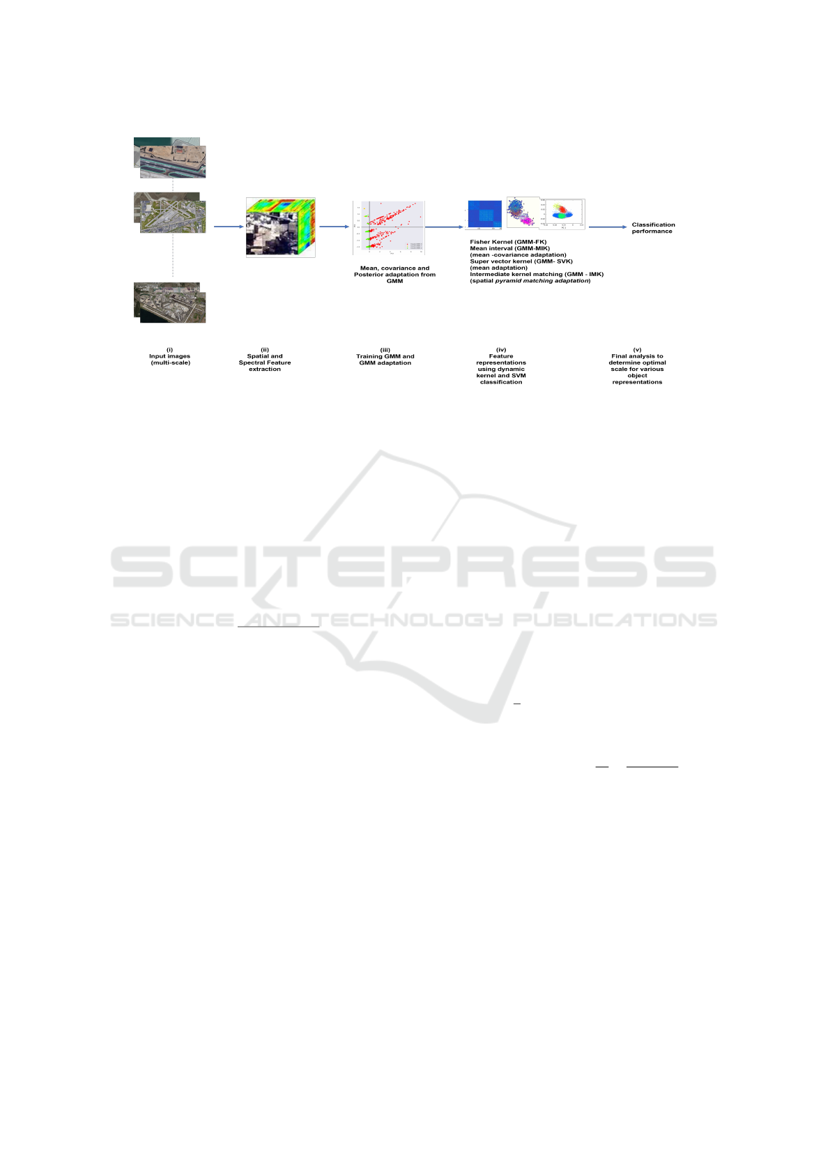
Figure 1: Block diagram for the proposed method to ﬁnd the optimum scale range for object representations using dynamic

kernels for Airport surveillance.

to distribution z. In the Maximization step, the pa-

rameters θ is updated using the values estimated in

the previous step.

The attributes and the variances in the spatial pat-

terns are captured in the Gaussian components after

the training phase. This helps in comparing the dif-

ferent images improving intra-class variability. Each

of the feature vectors i

is aligned to the k

compo-

nent of the Gaussian mixture model using the poste-

rior probabilities and is deﬁned as in Eqn. (3).

p(k|i

) =

p(i

|k)

∑

k=1

p(i

|k)

(3)

The maximum aposteriori (MAP) adaptation

helps in generating multiple dynamic kernel-based

representations, that can efﬁciently represent each of

the images. These representations are further detailed

in the subsequent sections.

3.3 Feature Representations Using

Dynamic Kernels

Identifying the right kernel function for feature rep-

resentations is critical to obtain a good performance.

In the earlier days, multiple kernel functions are de-

veloped for the static or ﬁxed-length pattern. In recent

years, researchers have discussed the dynamic kernels

built to address variable length patterns by designing a

new kernel function or converting the variable length

to ﬁxed length patterns. In this section, we detail the

various dynamic kernel functions that effectively pre-

serve both local and global information for better fea-

ture representations.

3.3.1 Mapping Based Dynamic Kernel

This method uses a Gaussian mixture model-based

likelihood to explicitly map a set of variable length

representations onto a ﬁxed dimensional representa-

tion. To obtain the maximum likelihood estimate of

the parameter θ, we calculate the derivative or gradi-

ent of the log-likelihood function deﬁned in Eqn. (3)

for a given image I. The ﬁrst derivatives of mean,

covariance, and weight parameters are deﬁned as in

Eqn. (4), Eqn. (5), and Eqn. (6), respectively.

(µ)

(I) =

∑

j=1

p(k|i

(4)

(σ)

(I) =

∑

j=1

p(k|i

)



−(x

) + y



(5)

(π)

(I) =

∑

j=1

p(k|i

)



−

p(k

)

p(k|i

)



(6)

where,

∑

−1

− µ

), x

∑

−1

, y

j1k

, r

j2k

, ..., r

jdk

] for any d × d ma-

trix A with elements a

i j

, i, j = 1, 2, ..., d and

vec(A) = [a

, a

, ..., a

The Eqn. (4), Eqn. (5), and Eqn. (6) determines

the direction of the parameters (µ, σ, π). These gra-

dients are updated to obtain the best ﬁt of the model.

The gradients capture the deviations introduced in the

objects due to spatial variability. The Fisher score

vector, which is the ﬁxed dimensional feature vec-

tor is computed by stacking the gradients from the

Eqn. (4), Eqn. (5), and Eqn. (6).

Quantitative Analysis to Find the Optimum Scale Range for Object Representations in Remote Sensing Images

373

(I) =

(µ)

(I)

, ψ

(σ)

(I)

, ψ

(π)

(I)

(7)

The Fisher score vector, for all the K components

of the GMM for a given space s, is given by the

Eqn. (8).

(I) =



(I)



(8)

The similarities between the two samples I

and

with given local features, is captured by the Fisher

score vector and the kernel function is given by the

Eqn. (9).

, I

) = φ

)

−1

)

(9)

where F is the Fisher information matrix which

is the covariance in the Mahanolibis distance and is

given by the Eqn. (10).

F =

∑

d=1

)φ

)

(10)

The spatial variability between two image samples

is captured in the Fisher information matrix. Fisher

score and Fisher information matrix, thus capture

both the local and global information in the Fisher

kernel computation. However, the Fisher Kernel ap-

proach is computationally expensive.

3.3.2 Probability Based Kernel Functions

The probability-based kernel functions compare the

probability distribution of the local feature vectors

of two images. In this method, the set of variable

length local feature representations are mapped onto

ﬁxed dimensional feature representations in the kernel

space using the probabilities. The maximum aposte-

rior (MAP) adaptation of mean and covariances are

calculated as given in the Eqn. (11a) and Eqn. (11b),

respectively.

(I) = αF

+ (1 −α)µ

(11a)

(I) = αS

(I) + (1 −α)σ

(11b)

where F

and S

are the ﬁrst and second-order Baum-

Welch statistics for an image I, respectively, and is

calculated as in Eqn. (12a) and Eqn. (12b), respec-

tively.

(I) =

(I)

∑

m=1

p(k|i

(12a)

(I) = diag

∑

m=1

p(k|i

)

(12b)

The posterior probabilities of the given GMM

component for each of the image samples are deter-

mined by the adapted mean and covariance. It is also

observed that the posterior probabilities are directly

dependent on the adapted mean and covariance, im-

plying, that the higher the probability higher is the

correlation among the features captured in the GMM

components. Thus, indicating that the adapted mean

and covariances have a higher impact than the original

full GMM mean and covariance. We further derive

the GMM vector ψ

(I) for an image I as in Eqn. (13).

(I) =



√

−1

(I)



(13)

The GMM super vector (GMM-SV) and the su-

per vector kernel S

svk

(I) and K

svk

, I

) as deﬁned

in Eqn. (14a) and Eqn. (14b), respectively, is obtained

by stacking the GMM vector for each component. We

obtain a supervector of Kd ×1 dimension that utilizes

the ﬁrst order adaptations.

svk

(I) =



(I)

, ψ

(I)

, ..., ψ

(I)



(14a)

SV K

, I

) = S

svk

)

svk

)

(14b)

In the super vector kernel method, we only utilize

ﬁrst order statistics of the GMM. To obtain the mean

interval vector for every component k of the GMM,

the second order statistics and the adapted means is

used as in Eqn. (15a). This help determine the statis-

tical dissimilarities between the mean and covariance

of the mean interval vector. The GMM mean interval

supervector is created by combining the mean inter-

val vectors across GMM mixtures S

mik

and the asso-

ciated GMM mean interval kernel K

MIK

between two

images I

and I

and is as given by Eqn. (15b) and

Eqn. (15c), respectively.

(I) =



(I) −σ



−1

(µ

(I) −µ

)

(15a)

mik

(I) =



(I)

, ψ

(I)

, ...ψ

(I)



(15b)

MIK

, I

) = S

mik

)

mik

)

(15c)

3.3.3 Matching Based Kernel Functions

The mapping-based and probability-based kernel

methods are based on mapping the feature represen-

tations from a variable to a ﬁxed length. An alternate

VISAPP 2023 - 18th International Conference on Computer Vision Theory and Applications

374

method to handle variable data lengths also known as

matching-based kernels is introduced in this section.

In this method, a pair of images is matched using their

local features (Datla et al., 2021) vectors. We use an

intermediate matching kernel (IMK) function that is

calculated using both the local feature vector and the

virtual feature vector. The virtual feature vectors are

obtained using the training data and are the closest

match to a set of local features. The feature vectors

∗

and i

∗

in I

and I

closest to the l

virtual feature

vector q

is given by the Eqn. (16).

∗

= arg min

i∈I

D (i, q

) and i

∗

= arg min

i∈I

D (i, q

)

(16)

where Q =

{

, q

, ...q

}

represents the virtual

feature vectors and D (., .) measures the distance be-

tween the feature vectors I

or I

from the nearest fea-

ture vector in Q. The distance function helps in identi-

fying the closest matching point and hence the spatial

distance learned from one image to another, which is

captured by the GMM components. The kernel func-

tion K

IMK

is given by Eqn. (17).

IMK

, I

) =

∑

l=1

k (i

, i

)

(17)

The set of virtual feature vectors also includes the

mean, covariance, and the weights. The posterior

probability of the GMM component determines the

distance, thus computing the virtual feature vectors

∗

and i

∗

for a given l for the image samples I

or I

as in Eqn. (18).

∗

= arg max

i∈I

p(l|i) and i

∗

= arg max

i∈I

p(l|i)

(18)

3.4 Classiﬁcation and Optimum Scale

Range Analysis

In the next phase, we implement the Support Vector

Machine (SVM) for the classiﬁcation task, for each

of the dynamic kernels. The support vector algo-

rithm helps determine a hyperplane between differ-

ent classes. Based on the dynamic kernel function

selected, we maximize the separation boundaries be-

tween the data points. For multi-class classiﬁcation,

we use the one vs. all approach to ﬁnd the hyperplane

to separate the classes. We use N support vector ma-

chines to classify data points from N class data sets.

For R training samples (I

, y

)

r=1

, where the label for

a particular class is represented by y

and the discrim-

inant function is given by the Eqn. (19),

f (I) =

∑

r=1

∗

(I, I

) + bias

∗

(19)

where R

represents the number of support vec-

tors, the optimal values of the Lagrangian coefﬁcient

is given by α

∗

and bias

∗

represents the optimal bias.

The class of I is determined by the sign of the func-

tion f . The 10-fold cross-validation helps discrimi-

nate the sample of the particular class against all other

classes. Further, we determine the correlation values

for various classes at different spatial distances. This

helps determine optimal range for the object represen-

tations.

4 EXPERIMENTAL RESULTS

AND ANALYSIS

The objective of our method is to identify the opti-

mum scale range for object representations that aids

in better airport surveillance. In this section, we dis-

cuss in detail the experimental results of applying

various dynamic kernel functions, namely, mapping

based, probability based and matching based kernels

on our custom dataset.

4.1 Datasets and Environmental Setup

Vision-based airport surveillance is challenging due

to non-availability of appropriate datasets. The com-

monly available remote sensing dataset is the NWPU-

RESISC45 (Cheng et al., 2017) that is design for the

classiﬁcation tasks. This dataset consists of 45 scenes

with a mix of 31,500 images with spatial range of

0.2m to 30m. The images are sized to 256 ×256 pix-

els each. These images fail to provide the relevant

statistics based on the spatial distance.

Therefore, a custom dataset is developed by

capturing images from NWPU-RESISC45 (Cheng

et al., 2017), different public repositories and

from GoogleEarth™ at different spatial resolutions -

0.125m (Scale - 1:500), 0.25m (Scale - 1:1000), and

0.5m (Scale - 1:2000) to obtain a realistic view of the

dataset. The ﬁnal airport object dataset is created with

six object categories, namely, vehicles, airplanes, run-

way, building, freeway, and parking lot.

The sample dataset is as shown in Figure 2. The

objects of interest are labeled using the polygon anno-

tation. A bounding box (x

, y

, x

, y

) is drawn using

the polygon points where (x

, y

) and (x

, y

) repre-

sents the top-left and bottom-right coordinates using

manual process and AI-enabled annotation tool.

The model is implemented using an NVIDIA

GeForce RTX 2060 Super EX (1-Click OC) with

CUDA cores 2176 and an 8GB GDDR6 256-bit

DP/HDMI. The proposed method is developed using

Quantitative Analysis to Find the Optimum Scale Range for Object Representations in Remote Sensing Images

375

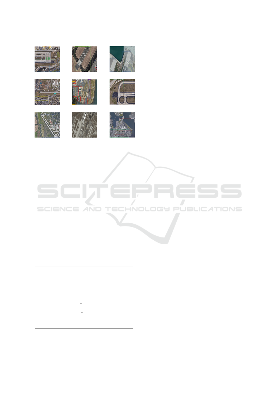
(a) SS05: Spatial Resolution - 0.125m.

(b) SS10: Spatial Resolution - 0.25m.

Figure 2: Airport Object Dataset: (a) SS05 : Spatial Reso-

lution - 0.125m (b) SS10 : Spatial Resolution - 0.25m (c)

SS20: Spatial Resolution - 0.5m.

open-source frameworks Keras, OpenCV, and Tensor-

Flow.

We use different convolutional features of vari-

ous convolutional neural networks (CNNs), namely,

AlexNet (Krizhevsky et al., ), GoogLeNet (Szegedy

et al., 2015), VGGNet-16 (Simonyan and Zisserman,

2014), DenseNet-121 (Huang et al., 2017), ResNet-

50 (He et al., 2016), and EfﬁcientNet-B0 (Tan and Le,

2019) as shown in Table 1 for extraction of both lo-

cal and global feature vectors for GMM training. We

train a total of 24 GMMs, i.e, features from six convo-

lutional neural network models for four mixtures on

three dataset combinations from the custom dataset.

Table 1: Feature map sizes of various CNN Architectures

used for object representation modeling.

Architecture Feature Layer Feature Map Size

AlexNet conv5 13 ×13 ×256

GoogLeNet inception 4(e) 14 ×14 ×832

VGGNet-16 block5 conv3 13 ×13 ×256

DenseNet-121 conv4 block16 7 ×7 ×1024

ResNet-50 conv5 block4 7 ×7 ×2048

EfﬁcientNet-B0 top conv 7 ×7 ×1280

4.2 Dynamic Kernel Evaluations

The performance of various dynamic kernels on our

custom dataset that is distributed based on the spatial

resolutions 1:500, 1:1000, and 1:2000 is as shown in

Table 2, Table 3, and Table 4, respectively. The clas-

siﬁcation performance is evaluated using support vec-

tor machine. The experimental results indicate that

the performance is best observed with the features ex-

tracted using EfﬁcientNet-B0 followed by ResNet-50

and DenseNet-121 for different GMM mixtures and

datasets. We also observe that as the number of com-

ponents increases, the accuracy comes to a close satu-

ration. As shown in the Table 2, Table 3, and Table 4,

for a GMM mixture with 128 components, the accu-

racy is less as compared to that of 64 component. The

results also indicate that classiﬁcation performance

is better with supervector kernels (GMM-SVK) and

mean interval kernels (GMM-MIK) compared to the

ﬁsher kernel (GMM-FK) and intermediate matching

kernel (GMM-IMK).

4.3 Scale Effect Analysis

The scale-effect analysis is evaluated by measuring

the Pearson correlation coefﬁcient. The input features

provide insight into the relationships between differ-

ent object classes for each of the subset datasets SS05,

SS10, and SS20.

SS05 dataset: The best classiﬁcation accuracy of

96.89% is achieved for 128 components using GMM-

MIK as shown in Table 2. From the Figure 3a, at a

scale of 0.125m, we observe the following:

• High correlation between freeway and runways,

• Vehicles have a high correlation with buildings

and parking lots.

• Airplanes are best classiﬁed at this range due to

low correlations.

SS10 dataset: The best classiﬁcation accuracy of

97.65% is achieved for 64 components using GMM

-MIK as shown in Table 3. From Figure 3b, at a scale

of 0.25m, we observe that all objects are less corre-

lated and better classiﬁed.

SS20 dataset:The best classiﬁcation accuracy of

95.32% is achieved for 64 components using GMM-

MIK as shown in Table 4. From Figure 3c, at a scale

of 0.5m, we observe that there is at least one pair of

objects highly correlated which makes the classiﬁca-

tion tasks difﬁcult to achieve.

VISAPP 2023 - 18th International Conference on Computer Vision Theory and Applications

376

Table 2: Classiﬁcation accuracy (%) of various GMMS- GMM-FK, GMM-SVK, GMM-MIK, GMM-IMK over GMM mix-

tures on SS05 subset dataset.

CNN

Model

AlexNet GoogLeNet VGGNet-16 DenseNet-121 ResNet-50 EfﬁcientNet-50

GMM -FK

GMM

Mixtures

16 45.42 48.21 47.63 51.28 40.53 44.32

32 48.34 48.18 48.72 54.63 51.74 55.45

64 47.91 48.61 49.51 53.45 52.87 56.73

128 47.66 48.98 49.45 52.55 51.46 54.83

GMM -SVK

GMM

Mixtures

16 81.65 82.47 88.69 90.35 94.27 95.32

32 82.41 83.49 88.72 94.53 95.43 96.37

64 84.32 86.33 89.25 94.82 95.65 95.41

128 84.66 87.29 89.86 96.76 95.23 96.34

GMM -MIK

GMM

Mixtures

16 78.26 80.24 81.23 91.92 93.43 94.56

32 79.32 79.27 83.46 88.72 92.35 96.73

64 79.17 81.54 83.91 94.97 95.27 95.23

128 78.93 82.34 82.68 93.28 95.66 96.89

GMM -IMK

GMM

Mixtures

16 62.57 67.14 69.23 74.18 66.17 75.12

32 62.49 69.2 69.56 75.22 75.67 76.45

64 64.18 69.46 69.64 74.76 76.34 77.45

128 66.62 68.87 69.25 75.33 76.2 77.28

Table 3: Classiﬁcation accuracy (%) of various GMMS- GMM-FK, GMM-SVK, GMM-MIK, GMM-IMK over GMM mix-

tures on SS10 subset dataset.

CNN

Model

AlexNet GoogLeNet VGGNet-16 DenseNet-121 ResNet-50 EfﬁcientNet-50

GMM -FK

GMM

Mixtures

16 47.35 51.76 52.63 52.35 51.33 55.21

32 47.76 53.23 51.25 63.43 61.65 65.78

64 46.34 51.34 52.45 64.57 63.56 66.24

128 48.66 52.54 51.23 64.23 62.49 65.32

GMM -SVK

GMM

Mixtures

16 77.26 83.36 83.56 92.23 94.76 95.12

32 78.87 81.34 81.56 94.34 93.67 95.45

64 78.32 82.75 82.78 94.23 94.98 96.89

128 79.24 83.24 83.23 93.22 94.32 96.32

GMM -MIK

GMM

Mixtures

16 80.34 86.56 87.54 91.76 95.19 95.32

32 82.67 85.45 87.65 92.99 94.8 97.32

64 83.87 85.65 88.34 95.87 95.34 97.65

128 83.44 87.65 87.25 95.92 95.67 95.36

GMM -IMK

GMM

Mixtures

16 66.36 65.56 68.65 75.43 75.34 75.33

32 69.39 68.56 67.34 76.34 76.36 76.76

64 68.38 69.34 66.78 76.23 77.1 77.98

128 67.56 69.34 68.43 76.76 77.14 77.65

Table 4: Classiﬁcation accuracy (%) of various GMMS- GMM-FK, GMM-SVK, GMM-MIK, GMM-IMK over GMM mix-

tures on SS20 subset dataset.

CNN

Model

AlexNet GoogLeNet VGGNet-16 DenseNet-121 ResNet-50 EfﬁcientNet-50

GMM -FK

GMM

Mixtures

16 45.35 47.62 47.12 51.33 58.45 59.23

32 48.77 57.92 57.34 52.34 59.25 59.43

64 49.54 47.45 48.34 51.76 58.14 53.42

128 40.23 47.87 48.23 53.34 52.45 51.78

GMM -SVK

GMM

Mixtures

16 76.65 79.35 79.13 83.16 89.98 93.87

32 78.24 80.23 80.21 84.33 90.24 94.23

64 76.33 80.87 81.22 85.45 91.34 94.85

128 76.65 84.32 81.45 86.13 92.42 94.44

GMM -MIK

GMM

Mixtures

16 79.82 83.56 83.32 85.66 92.32 95.28

32 80.34 84.21 84.55 85.34 93.56 95.18

64 81.52 85.43 84.78 86.67 93.38 95.32

128 80.11 85.92 85.34 86.89 94.56 95.28

GMM -IMK

GMM

Mixtures

16 66.54 76.23 73.34 76.54 85.87 85.43

32 68.65 75.36 73.67 76.78 85.92 85.16

64 69.32 75.32 74.34 77.43 85.45 86.56

128 69.45 75.56 74.87 77.29 86.34 84.29

Quantitative Analysis to Find the Optimum Scale Range for Object Representations in Remote Sensing Images

377

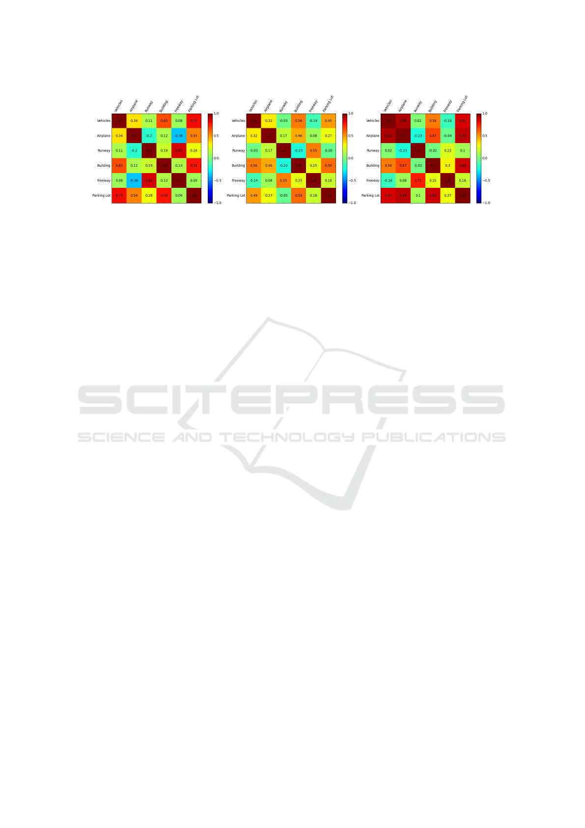
(a) SS05 subset dataset. (b) SS10 subset dataset. (c) SS20 subset dataset.

Figure 3: Correlation matrix of GMM-MIK for (a) SS05 subset dataset (b) SS10 subset dataset (c) SS20 subset dataset.

5 CONCLUSIONS

In this work, we introduce the use of dynamic ker-

nels to ﬁnd the optimum scale range for object repre-

sentations in remote-sensing images. For this, we ex-

ploit multiple dynamic kernels, namely, Fisher Kernel

(GMM-FK), Intermediate Matching Kernel (GMM-

IMK), Mean Interval Kernel (GMM-MIK), and Su-

per Vector Kernel (GMM-SVK) methods. The scale

effect analysis is evaluated using the ﬁrst- and second-

order statistics of the Gaussian mixture model. The

Gaussian mixture models allow capturing spatial and

object variability while continuing to preserve the

global variance. Our analysis indicates that the mean

interval kernel method (GMM-MIK) is most suitable

for the classiﬁcation task. We introduce a custom

dataset consisting of images at different spatial ranges

to evaluate the performance of our method. In the fu-

ture, the method needs to be optimized to ﬁnd a closer

range of optimum values for object representations.

The method also needs to be expanded to evaluate ad-

ditional object classes to reﬂect the real-time environ-

ment.

REFERENCES

Akbar, J., Shahzad, M., Malik, M. I., Ul-Hasan, A., and

Shafait, F. (2019). Runway detection and localization

in aerial images using deep learning. In 2019 Dig-

ital Image Computing: Techniques and Applications

(DICTA), pages 1–8. IEEE.

Artan, G. A., Neale, C. M., and Tarboton, D. G. (2000).

Characteristic length scale of input data in distributed

models: implications for modeling grid size. Journal

of Hydrology, 227(1-4):128–139.

Boughorbel, S., Tarel, J. P., and Boujemaa, N. (2005). The

intermediate matching kernel for image local features.

In Proceedings. 2005 IEEE International Joint Con-

ference on Neural Networks, 2005., volume 2, pages

889–894. IEEE.

Burghouts, G. J. and Geusebroek, J.-M. (2009). Perfor-

mance evaluation of local colour invariants. Computer

Vision and Image Understanding, 113(1):48–62.

Cheng, G., Han, J., Guo, L., and Liu, T. (2015a). Learning

coarse-to-ﬁne sparselets for efﬁcient object detection

and scene classiﬁcation. In Proceedings of the IEEE

conference on computer vision and pattern recogni-

tion, pages 1173–1181.

Cheng, G., Han, J., Guo, L., Liu, Z., Bu, S., and Ren,

J. (2015b). Effective and efﬁcient midlevel visual

elements-oriented land-use classiﬁcation using vhr re-

mote sensing images. IEEE Transactions on Geo-

science and Remote Sensing, 53(8):4238–4249.

Cheng, G., Han, J., and Lu, X. (2017). Remote sensing

image scene classiﬁcation: Benchmark and state of

the art. Proceedings of the IEEE, 105(10):1865–1883.

Cheng, G., Han, J., Zhou, P., and Guo, L. (2014). Multi-

class geospatial object detection and geographic im-

age classiﬁcation based on collection of part detectors.

ISPRS Journal of Photogrammetry and Remote Sens-

ing, 98:119–132.

Cheng, G., Yang, C., Yao, X., Guo, L., and Han, J. (2018).

When deep learning meets metric learning: Remote

sensing image scene classiﬁcation via learning dis-

criminative cnns. IEEE transactions on geoscience

and remote sensing, 56(5):2811–2821.

Cheng, G., Zhou, P., Han, J., Guo, L., and Han, J. (2015c).

Auto-encoder-based shared mid-level visual dictio-

nary learning for scene classiﬁcation using very high

resolution remote sensing images. IET Computer Vi-

sion, 9(5):639–647.

Datla, R., Chalavadi, V., et al. (2021). Scene classiﬁcation

in remote sensing images using dynamic kernels. In

2021 International Joint Conference on Neural Net-

works (IJCNN), pages 1–8. IEEE.

Garrigues, S., Allard, D., Baret, F., and Weiss, M. (2006).

Quantifying spatial heterogeneity at the landscape

scale using variogram models. Remote sensing of en-

vironment, 103(1):81–96.

Geusebroek, J.-M., Van den Boomgaard, R., Smeulders, A.

W. M., and Geerts, H. (2001). Color invariance. IEEE

Transactions on Pattern analysis and machine intelli-

gence, 23(12):1338–1350.

VISAPP 2023 - 18th International Conference on Computer Vision Theory and Applications

378

He, K., Zhang, X., Ren, S., and Sun, J. (2016). Deep resid-

ual learning for image recognition. In Proceedings of

the IEEE conference on computer vision and pattern

recognition, pages 770–778.

He, N., Fang, L., Li, S., Plaza, A., and Plaza, J. (2018).

Remote sensing scene classiﬁcation using multilayer

stacked covariance pooling. IEEE Transactions on

Geoscience and Remote Sensing, 56(12):6899–6910.

Huang, G., Liu, Z., Van Der Maaten, L., and Weinberger,

K. Q. (2017). Densely connected convolutional net-

works. In Proceedings of the IEEE conference on

computer vision and pattern recognition, pages 4700–

4708.

Jackson, P. T., Nelson, C. J., Schiefele, J., and Obara, B.

(2015). Runway detection in high resolution remote

sensing data. In 2015 9th International Symposium

on Image and Signal Processing and Analysis (ISPA),

pages 170–175. IEEE.

Krizhevsky, A., Sutskever, I., and Hinton, G. E. Imagenet

classiﬁcation with deep convolutional neural networks

(alexnet) imagenet classiﬁcation with deep convolu-

tional neural networks (alexnet) imagenet classiﬁca-

tion with deep convolutional neural networks.

Lee, K.-A., You, C., Li, H., and Kinnunen, T. (2007). A

gmm-based probabilistic sequence kernel for speaker

veriﬁcation. In Eighth Annual Conference of the In-

ternational Speech Communication Association. Cite-

seer.

Ming, D., Li, J., Wang, J., and Zhang, M. (2015). Scale pa-

rameter selection by spatial statistics for geobia: Us-

ing mean-shift based multi-scale segmentation as an

example. ISPRS Journal of Photogrammetry and Re-

mote Sensing, 106:28–41.

Moellering, H. and Tobler, W. (1972). Geographical vari-

ances. Geographical analysis, 4(1):34–50.

Nogueira, K., Penatti, O. A., and Dos Santos, J. A. (2017).

Towards better exploiting convolutional neural net-

works for remote sensing scene classiﬁcation. Pattern

Recognition, 61:539–556.

Pelgrum, H. (2000). Spatial aggregation of land surface

characteristics: impact of resolution of remote sens-

ing data on land surface modelling. Wageningen Uni-

versity and Research.

Pi, Y., Fan, L., and Yang, X. (2003). Airport detection

and runway recognition in sar images. In IGARSS

2003. 2003 IEEE International Geoscience and Re-

mote Sensing Symposium. Proceedings (IEEE Cat.

No. 03CH37477), volume 6, pages 4007–4009. IEEE.

Simonyan, K. and Zisserman, A. (2014). Very deep con-

volutional networks for large-scale image recognition.

arXiv preprint arXiv:1409.1556.

Sitaula, C., Xiang, Y., Basnet, A., Aryal, S., and Lu, X.

(2020). Hdf: Hybrid deep features for scene image

representation. In 2020 International Joint Confer-

ence on Neural Networks (IJCNN), pages 1–8. IEEE.

Szegedy, C., Liu, W., Jia, Y., Sermanet, P., Reed, S.,

Anguelov, D., Erhan, D., Vanhoucke, V., and Rabi-

novich, A. (2015). Going deeper with convolutions.

In Proceedings of the IEEE conference on computer

vision and pattern recognition, pages 1–9.

Tan, M. and Le, Q. (2019). Efﬁcientnet: Rethinking model

scaling for convolutional neural networks. In Interna-

tional conference on machine learning, pages 6105–

6114. PMLR.

Van De Sande, K., Gevers, T., and Snoek, C. (2009). Eval-

uating color descriptors for object and scene recogni-

tion. IEEE transactions on pattern analysis and ma-

chine intelligence, 32(9):1582–1596.

Wackernagel, H. (1996). Multivariate geostatistics: an in-

troduction with applications. In International Journal

of Rock Mechanics and Mining Sciences and Geome-

chanics Abstracts, volume 8, page 363A.

Woodcock, C. E. and Strahler, A. H. (1987). The factor of

scale in remote sensing. Remote sensing of Environ-

ment, 21(3):311–332.

Yang, Y. and Newsam, S. (2008). Comparing sift descrip-

tors and gabor texture features for classiﬁcation of re-

mote sensed imagery. In 2008 15th IEEE interna-

tional conference on image processing, pages 1852–

1855. IEEE.

You, C. H., Lee, K. A., and Li, H. (2009). Gmm-svm ker-

nel with a bhattacharyya-based distance for speaker

recognition. IEEE Transactions on Audio, Speech,

and Language Processing, 18(6):1300–1312.

Quantitative Analysis to Find the Optimum Scale Range for Object Representations in Remote Sensing Images

379