Implicit Cooperative Learning on Distribution of Received Reward in
Multi-Agent System
Fumito Uwano
a
Department of Computer Science, Okayama University, 3-1-1, Tsushima-naka, Kita-ku, Okayama, Japan
Keywords:
Multiagent System, Reinforcement Learning, Neural Network, Implicit Learning, Normal Distribution.
Abstract:
Multi-agent reinforcement learning (MARL) makes agents cooperate with each other by reinforcement learn-
ing to achieve collective action. Generally, MARL enables agents to predict the unknown factor of other
agents in reward function to achieve obtaining maximize reward cooperatively, then it is important to diminish
the complexity of communication or observation between agents to achieve the cooperation, which enable it
to real-world problems. By contrast, this paper proposes an implicit cooperative learning (ICL) that have an
agent separate three factors of self-agent can increase, another agent can increase, and interactions influence
in a reward function approximately, and estimate a reward function for self from only acquired rewards to
learn cooperative policy without any communication and observation. The experiments investigate the perfor-
mance of ICL and the results show that ICL outperforms the state-of-the-art method in two agents cooperation
problem.
1 INTRODUCTION
Multiagent Reinforcement Learning (MARL) con-
trols some agents in groups to learn cooperative ac-
tion, such as in warehouses where robot agents coop-
erate with each other to manage the delivery of sup-
plies. In this case, MARL must decrease the complex-
ity of communication to achieve the desired coopera-
tion and enable the robots to solve real-world prob-
lems. In previous work, Kim et al. discussed a practi-
cal scenario for each agent to communicate with other
agents in real-world reinforcement learning tasks and
proposed a multiagent deep reinforcement learning
(DRL) framework called SchedNet (Kim et al., 2019).
Du et al. expanded the focus to the dynamic na-
ture of communication and the correlation between
agents’ connections to propose a learning method to
obtain the topology (Du et al., 2021). Those works
are efficient and straightforward, but the agents them-
selves cannot do complex tasks based on real-world
problems, especially in a dynamic environment. In
contrast, Raileanu et al. proposed self–other model-
ing (SOM) method to enable agents to learn coopera-
tive policy through predicting others’ purpose or goals
based only on the observation (Raileanu et al., 2018).
Ghosh et al. argued that the premise of SOM requires
a
https://orcid.org/0000-0003-4139-2605
the behaviors and types of all agents be presented as
a problem and proposed AdaptPool and AdaptDQN
as cooperative learning methods without using this
premise (Ghosh et al., 2020). However, the proposed
framework rely on the conception of step to make
agents learn synchronously. It is hard to apply it for
real-world problem.
Given this background, this paper proposes Im-
plicit cooperative learning (ICL) method to enable
agents to learn collective actions based on only re-
ward signal calculation. In particular, the ICL method
in which agents learn cooperative policy by estimat-
ing their appropriate reward to decrease an influence
to the other agent implicitly. This paper also com-
pared the ICL method with its baseline method and
the SOM in a fully cooperative task to validate the
effectiveness of the ICL method.
This paper is organized as follows: In Section 2,
we introduce the background technique: the structure
of game, the A3C and SOM. In Section 3, we describe
the ICL method and the mathematical analysis. Fur-
thermore, the experimental details and discussions are
described in Section 4. Finally, the conclusions are
presented in Section 5.
Uwano, F.
Implicit Cooperative Learning on Distribution of Received Reward in Multi-Agent System.
DOI: 10.5220/0011593500003393
In Proceedings of the 15th International Conference on Agents and Artificial Intelligence (ICAART 2023) - Volume 1, pages 147-153
ISBN: 978-989-758-623-1; ISSN: 2184-433X
Copyright
c
 2023 by SCITEPRESS – Science and Technology Publications, Lda. Under CC license (CC BY-NC-ND 4.0)
147

2 BACKGROUND
2.1 Problem Formulation
We consider a decentralized Partially observable
Markov decision process (Dec-POMDP) M for two
agents, defined by the tuple (I ,S,A,O,O,T , r,γ).
There are a set of states S , a set of actions A, and
a set of observations O, and a transaction function
T : S ×A → S . The agents parcially perceive their
state by following the observation function O : S ×
A → O, and selects an action by the stochastic pol-
icy π
θ
i
: S ×A → [0,1] and receives a reward from a
reward function r : S ×A
i
→ R. The agent attempts
to maximize the accumulated reward R =
∑
T
t=0
γ
t
r
t
,
where γ is a discount factor and T is the time horizon.
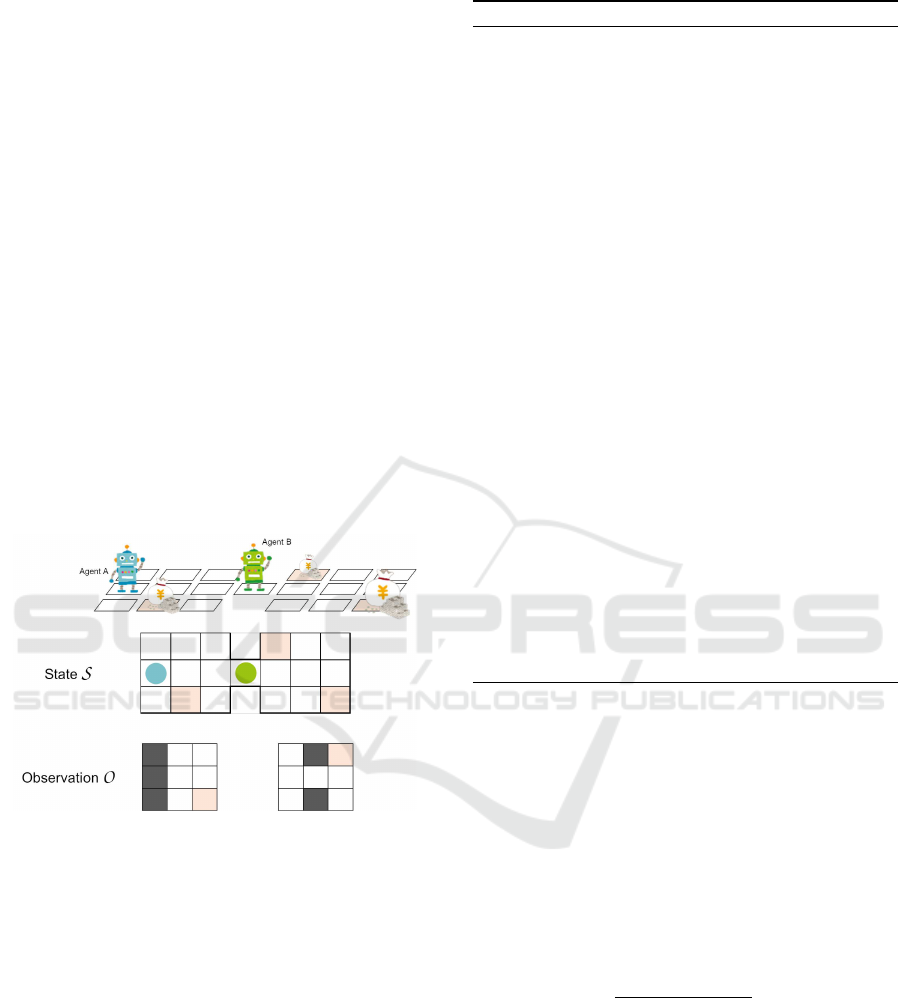
Figure 1 shows an example for description of the state
S and the observation O. The state S represents allo-
centric observation shown in the middle of the figure,
while the observation O represents egocentric obser-
vation, e.g., 8-neighboring features, in the bottom of
that. The agent can observe the portion of state s ∈O.
Figure 1: The problem formulation.
2.2 Asynchronous Advantage
Actor–critic
The A3C algorithm (Mnih et al., 2016) is a DRL
method where the system assigns the same learn-
ing components, agents, environments, and etc., into
some processes each other, and then executes trials
asynchronously to acquire an optimal policy imme-
diately. This paper descriptions the details of A3C
in (Fujita et al., 2019). The assigned agents execute
backpropagation to update the neural network of the
primary agent with the own loss of the parameters.
After that learning, they initialize themselves and up-
date the current parameters from that of the primary
network and repeat the processes.
Here, we show Algorithm 1, the pseudo code of
Algorithm 1: Algorithm of A3C.
Require: Initialize thread step counter t ← 1
1: while T > T
max
do
2: Reset gradients: dθ ←0 and dθ
v
← 0.
3: Synchronize thread-specific parameters θ
0
= θ
and θ
0
v
= θ
v
4: t
start
= t
5: Get state s
t
6: while terminal s
t
or t −t
start
== t
max
do
7: Perform a
t
according to policy π(a
t
|s
t
;θ
0
)
8: Receive reward r
t
and new state s
t+1
9: t ←t + 1
10: T ← T + 1
11: end while
12: R =

0 for terminal s
t
V (s
t
,θ
0
v
) for non-terminal s
t
13: for i ∈t −1,...,t
start
do
14: R ← r
i
+ γR
15: A(s
i
,a
i
;θ, θ
v
) =
∑
k−1
j=0
γ
j
r
i+ j
+
γ
k
V (s
i+k
;θ
v
) −V (s
i
;θ
v
)
16: Accumulate gradients wrt θ
0
: dθ ←
dθ + ∇
θ
0
logπ (a
i
|s
i
;θ
0
)A(s
i
,a
i
;θ, θ
v
) +
β∇
θ
0
H(π (s
i
;θ
0
))
17: Accumulate gradients wrt θ
0
v
: dθ
v
← dθ
v
+
∂(R −V (s
i
;θ
0
v
))
2
/∂θ
0
v
18: end for
19: Perform asynchronous update of θ using dθ
and of θ
v
using dθ
v
20: end while
A3C. Generally, state s or sensed information to de-
tect the state is input to the network and the policy π or
state–action value Q(s,a) is output from the network
in DRL. A3C approximates the policy π(a
t
|s
t
;θ) and
the state value V (s
t
;θ
0
v
) appropriately throughout the
entire processes. In particular, A3C updates the net-
work parameters by following equations (the 16th and
17th lines in Algorithm 1):
dθ ←dθ + ∇
θ
0
logπ

a
t
|s
t
;θ
0

A(s
t
,a
t
;θ, θ
v
)
+ β∇
θ
0
H(π

s
t
;θ
0

), (1)
dθ
v
←dθ
v
+
∂(R −V (s
t
;θ
0
v
))
2
∂θ
0
v
, (2)
where the losses θ
0
and θ
0
v
in each process. There
is an arbitrary step i to labeled the state, action and
reward by s
i
, a
i
, and r
i
, respectively. the parameter
θ
0
is updated using the entropy function H(π(s
i
;θ
0
))
multiplied by the factor β. In the advantage function
A(s
i
,a
i
;θ, θ
v
), the calculation includes the future re-
ward multiplied by the discount factor γ.
ICAART 2023 - 15th International Conference on Agents and Artificial Intelligence
148

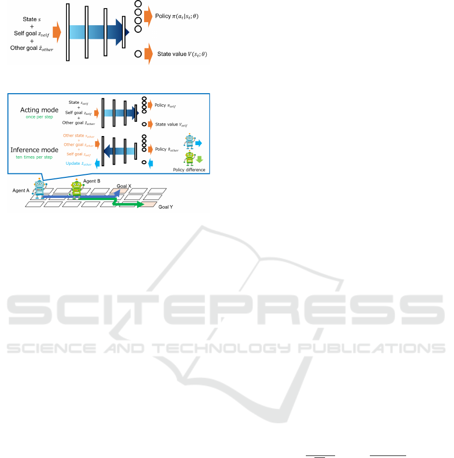
Figure 2: Neural network in SOM.
Figure 3: The process in SOM.
2.3 Self-Other Modeling (SOM)
The SOM enables an agent to estimate the other
agent’s goal by its neural network and input a self-
state, a self-goal, and the estimated goal to learn coop-
erative policy. Figure 2 shows an example of the SOM
model. This model learns from an observed state, the
self goal z
sel f
, and the self estimated other goal
e
z
other
,
involving backpropergation of the difference between
the estimated other agent’s behavior and the actual
one each step to update
e
z
other
.
Equation (3) denotes the neural network model as
approximation function in the SOM. The SOM esti-
mates parameter θ asymptotically.

π
V

= f (s
sel f
,z
sel f
,
e
z
other
;θ). (3)
Then, the SOM has two network models as follows:
f
sel f
(s
sel f
,z
sel f
,
e
z
other
;θ
sel f
) (4)
f
other
(s
other
,
e
z
other
,z
sel f
;θ
sel f
). (5)
The former is used for its learning and the latter is
used for estimating the other agent’s goal. Note that
the SOM uses the two with the same parameter θ
sel f
,
that is, the two is the same but the inputs are different
each other.
Figure 3 shows the process in the SOM in an ex-
ample of maze problem where two agents observe
their coordinates as portions of states and move with
four directions, up, down, left, and right. In this prob-
lem, the agents aim to reach the different goal each
other with the minimum number of steps. The SOM
has two modes called the acting mode and inference
mode. In the acting mode, the agent updates the pa-
rameter θ
sel f
using backpropergation of the loss based
on the reward and the output from the state s
sel f
and
the goals z
sel f
and z
other
every step in each episode.
In the inference mode, the agent outputs the esti-
mated other policy
e
z
other
to update the other agent’s
goal
e
z
other
using backpropergation with the actual ac-
tion ten times for ever step. Note that the number of
processing the inference mode can be changed rather
than 10, but this description is using 10 along to the
experiment in this paper.
The SOM has the complete information, e.g., the
other agent’s state. By contrast, the ICL method has
a neural network in which input only the self state
and the estimated goal to learn cooperative policy by
the internal reward without whole of the other goal
estimation.
3 IMPLICIT COOPERATIVE
LEARNING (ICL)
The ICL method enables an agent to avoid unexpected
interaction with the other agent to maximize the re-
ward function by maximizing a self-reward function.
The ICL method estimates the reward function as
standard normal distribution and divides the reward
function into two parts for an acquired reward and a
reward interfered with by the other agent. The ICL
method assumes that agents have the same strategy
each other implicitly and learn cooperative policy by
integration of both agents’ optimization.
3.1 Mechanisms
We replaced the acquired reward as a scalar to the
function as follows in the ICL:
f
g
(r) =
1
√
2πσ
g
exp −
(r −µ
g
)
2
2σ
2
g
!
, (6)
where the variables µ
g
and σ
g
denote a mean and a
standard deviation for the arbitrary goal g from the
rewards acquired throughout the entire episodes, re-
spectively. And then, the reward value is denoted by
r.
Figure 4 shows an example where two agents in
one maze with two goals as the same rules of Figure
2. The speech balloon represents the agent A’s inside
process with two reward functions estimated the own
parameters µ and σ. The agent proceeds estimating
the reward functions at the end of each episode. After
having acquired reward, the agent update the parame-
ters µ and σ for the corresponding goal. To update µ
Implicit Cooperative Learning on Distribution of Received Reward in Multi-Agent System
149

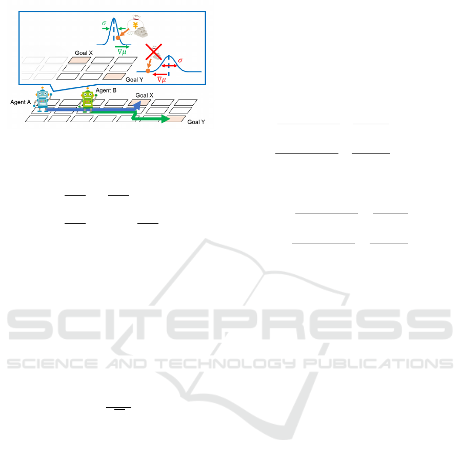
Figure 4: The mechanisms in ICL.
and σ recursively, the ICL method adopts the follow-
ing equations:
µ
n+1
←
n
n + 1
µ
n
+
x
n+1
n + 1
. (7)
σ
2
n+1
←
n
n + 1
(σ
2
n
+ µ
2
n
) +
x
2
n+1
n + 1
−µ
2
n+1
, (8)
where the variable n denotes a number of update.
This figure illustrates two cases: the agent A can
reach the goal X without any interference and cannot
reach the goal Y by the agent B’s interference. In the
former case, the agent A update the variables µ and σ
in the reward function for the goal X to shape it being
keen and narrowing. In the latter case, the agent A
cannot acquire any amount of reward to decrease the
average value µ and shape it dull.
For each learning part, the ICL method designs a
reward for each agent as shown in Equation (9). The
variable ir is an internal reward by which an agent
learn actually.
ir =
µ
√
2πσ
. (9)
The value of ir is on a peak of a normal distribution,
which an agent aims to decrease the standard devia-
tion σ and increase the averaged reward value µ. If
the other agent interferes with, the standard deviation
σ is decreased. Thus, the agent implies to learn ap-
propriate policy with avoiding the other agents each
other by maximizing the average reward value µ with
decreasing the standard deviation σ simultaneously.
3.2 Mathematical Analysis
We analyzed the ICL mechanisms in one condition
that the reward function can be separated by three
functions approximately shown as follows:
R(τ
sel f
,τ
other
) ≈ r(τ
sel f
) + r(τ
other
) + r
i
(τ
sel f
,τ
other
),
where R, r, and r
i
denote a total reward function and
reward functions for self and the other agents, and
their interaction, respectively. τ
sel f
and τ
other
denote
potential variables which can be routes, sequential
state-action pairs, etc. to represent the agents’ trajec-
tories and difference each other. However, this paper
adopts the trajectory, that is, the reward must be de-
cided based on the agents’ routes.
First, we derive the total derivative r
i
(τ
sel f
,τ
other
)
as follows:
dr
i
(τ
sel f
,τ
other
)
=

∂R(τ
sel f
,τ
other
)
∂τ
sel f
−
∂r(τ
sel f
)
∂τ
sel f

dτ
sel f
+

∂R(τ
sel f
,τ
other
)
∂τ
other
−
∂r(τ
other
)
∂τ
other

dτ
other
. (10)
If the derivative dr
i
(τ
sel f
,τ
other
) is zero, the following
two conditions are hold:
∂R(τ
sel f
,τ
other
)
∂τ
sel f
=
∂r(τ
sel f
)
∂τ
sel f
. (11)
∂R(τ
sel f
,τ
other
)
∂τ
other
=
∂r(τ
other
)
∂τ
other
. (12)
These conditions show the derivative values of the to-
tal reward function and the partial reward function are
the same each other in each agent’s potential vari-
able, that is, the influence of the total reward func-
tion is completely according to that of the partial re-
ward function. Therefore, the ICL method makes
an agent decrease a variance of a reward throughout
episodes to prevent from interception with the other
agent. Furthermore, the variance approximately is
zero, the derivative value dr
i
(τ
sel f
,τ
other
) is also zero.
4 EXPERIMENT
4.1 Experimental Setup
To investigate the effectiveness, this paper compared
the ICL method with the SOM and A3C in Coin
Game, respectively. The ICL method employed the
A3C algorithm based on (Fujita et al., 2019). The
evaluation criteria are the spent step until all agents
have reached the goal and the agents’ acquired re-
wards.
4.2 Coin Game
Coin Game (Raileanu et al., 2018) is a fully coopera-
tive task, which agents aim to gain maximum reward
when they have both of their goals rather than only
their goal. In this task, every agent is assigned of a
color of coin and its policy is evaluated by Equation
ICAART 2023 - 15th International Conference on Agents and Artificial Intelligence
150

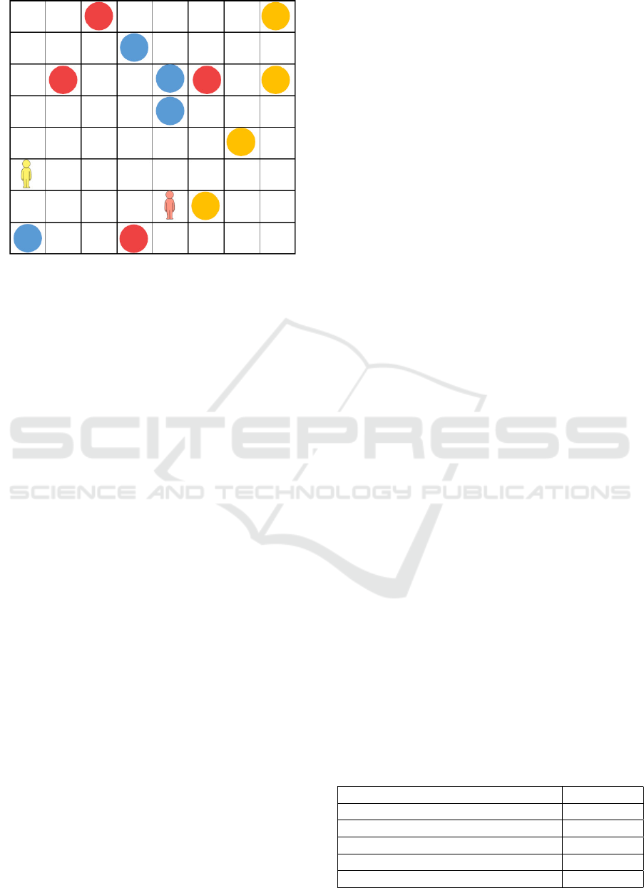
Figure 5: An example of Coin Game.
(13) as follows in the color assignment:
R
coin
=

n
sel f
C
sel f
+ n
other
C
sel f

2
+

n
sel f
C
other
+ n
other
C
other

2
−

n
sel f
C
neither
+ n
other
C
neither

2
, (13)
where R
coin
denotes a reward to share both of agents.
The words sel f and other indicate the agent which
actually gain the reward and the other agent, respec-
tively. Thus, C
sel f
and C
other
indicate the color of
coins assigned to sel f and other agents, respectively,
and n
sel f
C
sel f
, n
sel f
C
other
denote the numbers of coins as-
signed to the sel f and other agents in the coins gath-
ered by the sel f agent, respectively. The number
n
sel f
C
neither
denotes the number of coins assigned to no-
one in the coins gathered by the sel f agent. The num-
bers of coins n
other
C
sel f
, n
other
C
other
, and n
sel f
C
neither
are denoted in
the same manner of the sel f agent.
Figure 5 shows a circumstance of Coin Game in
one episode. There represent two humans as agents
and 12 circles as coins in a 8 ×8 grid world, and the
color of agents and coins shows the assigned colors.
The agents explore to gather the same color coins in
an entire episode and gain a reward at the end of the
episode. After that, the location and color of agents
and coins are changed and the agents go on to the
next episode. The agents are assigned of different
colors each other, and the colors are changed in each
episode in Coin Game. In the ICL method, let the
potential variable τ be a pair with assigned color and
self-gathered coins.
4.3 Training Details
The parameters are summarized on Table 1. Totally,
0.2 billion steps are executed (first line) and agents
learn up to 10 steps in one episode (second line). An
episode is finished within 10 steps if all coins have
been gathered. The number of processes is 16 (third
line). The parameters α, γ, and β are set by 0.0007,
0.99, and 0.01 (i.e., fourth, fifth, and sixth lines, re-
spectively). The total number of steps in an episode
and the number of processes are the same as SOM.
The ICL method’s neural network in which two
hidden layers, dense and LSTM layers. The dense
layer is connected from the input layer and connects
to the LSTM layer. The LSTM layer connects to two
output layers for a policy and a state value. The pa-
rameter optimization using Adam (Kingma and Ba,
2017). The hidden layer dimension was 64. The
network is the same as SOM. As for the input fea-
tures, there are seven features (two agents, three
coins, a wall and an empty state) in each of 64 grid
squares and the input has 448 features totally. There
are six features, less than ICL by one feature, in
(Raileanu et al., 2018), however ICL has ”nothing”
class whereas SOM classify it by decreasing all fea-
tures to zero, that is, both have the same features ac-
tually. By the way SOM has six features (two agents,
three coins, a corner.) Furthermore, there are addi-
tion input features show self and other colors (i.e., six-
dimension vector) in the SOM. The ICL has only self-
color as additional features with three dimensional
vector.
4.4 Results
Figure 6 shows the performance of ICL and A3C. The
vertical and horizontal axes indicate a total value of
reward and each episode, respectively. Both of the re-
sults are moving average in 10,000 episodes. This fig-
ure shows the ICL method outperforms the A3C and
the result converged to over 13. Figure 7 shows the
performance of the SOM and the other baseline meth-
ods as shown in (Raileanu et al., 2018). Although this
paper did not explain the detail of the other baseline
methods, the TOG, or the high performance method,
is not considered because it utilizes a given and opti-
mal values in a part of parameters. The vertical and
horizontal axes indicate a total value of reward and
each episode, respectively. The scale of episode in
ICL and A3C is decuple than SOM, however SOM
Table 1: Experimental parameters.
Total number of steps in all episodes 20,000,000
Total number of steps in an episode 10
Processes 16
Learning rate α 0.0007
Discount rate γ 0.99
Rate β 0.01
Implicit Cooperative Learning on Distribution of Received Reward in Multi-Agent System
151

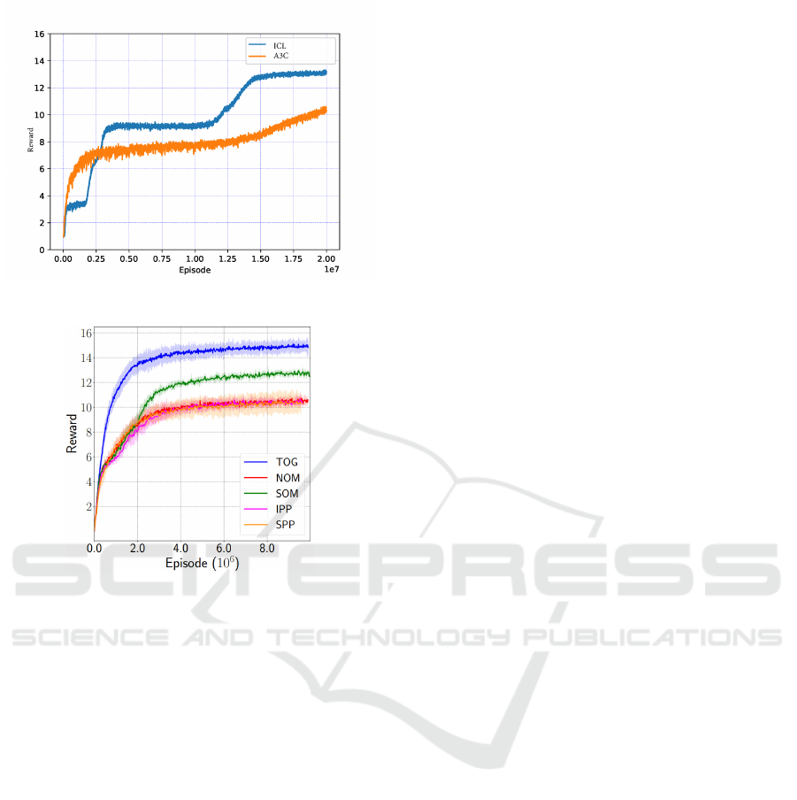
Figure 6: Coin performance in ICL and A3C.
Figure 7: Coin performance in SOM. (Raileanu et al.,
2018).
executes optimization update of its parameter for 10
times in every step. Thus actual scale is the same each
other and the number of ICL and A3C update parame-
ter is less than SOM. Each result is averaged in 5 runs
and the standard deviation is shown as the light color
area around the line. This figure shows the result of
SOM converged to under 13. That result is naturally
smaller than that of the ICL.
4.5 Discussion
4.5.1 Stability of Learning
The result of ICL method is moving average because
that is not stably by comparing that of the SOM. How-
ever, the difference of each framework, without learn-
ing performance, causes that effect. Concretely, that
is because the SOM enables agents to update their pa-
rameters for 10 times at each step, the trajectory is
stable in Figure 7. However, that seems to become
serious problem in real world. That is because there
is no conception of step. For example, there are two
robots in a warehouse. The robots carry supplies on to
the appropriate shelf and arrange them cooperatively.
In this circumstance, each agent makes a delay by
the update parameter. Thus, the SOM required agents
achieve synchronous actions.
That unstableness can be solved by the Maximum
entropy inverse reinforcement learning (MEIRL)
technique in (Ziebart et al., 2008). In particular, the
ICL utilizes the potential variable τ similar to the ex-
pert demonstration. That is one of the future works.
4.5.2 Convergence
The trajectory of the A3C and the SOM goes on in
smooth. However, that of the ICL goes on in steps.
That shows the ICL transited through three kinds of
equilibrium. In the first equilibrium, the agents gained
about three as a value of reward. In the next equi-
librium, the agents gained about nine in a long term.
That result suggests the agents can averagely gather
two coins. In the final equilibrium, the agents gained
about thirteen in which they can gather averagely two
and a half coins. The ICL avoid unstable policy which
causes a bad effect to an interaction between agents
and keeps a new valuable equilibrium, unlike other
methods. That is why the result of the ICL has small
variance and outperform than that of A3C.
4.5.3 Limitation
Agents should have gained 32 value of reward in Coin
Game. However, the ICL method could not achieve
that. That reason is the difference or lack of premise.
The result shows us right of the premise that the self-
reward function follows a normal distribution and the
influence of interaction could be in the standard de-
viation. However, a noise in the total reward cannot
always follow a normal distribution. In short, all of
the standard deviation do not represent the influence
of interaction. At least, a normal distribution cannot
represent change of the total reward function by the
other agent’s learning and that change is a part of the
standard deviation. The ICL has limitation in terms
of a premise of distribution.
To tackle this issue, there is a way in how to uti-
lize kernel density estimation. However, the compu-
tational complexity intercepts the ICL method. Thus,
the more suitable parametric distribution should be
considered in the future.
5 CONCLUSION
This paper proposed the ICL method in which agents
learn cooperative policy by estimating their appro-
priate reward to decrease an influence to the other
agent implicitly. Concretely, the ICL method makes
ICAART 2023 - 15th International Conference on Agents and Artificial Intelligence
152

an agent separate three partial reward functions for
self and the other agents, and an interaction with the
agents approximately, and estimates a reward func-
tion for self based on only acquired rewards to learn
without factors of the other agent and an interaction
with the other agent. The experiments compared the
ICL method with A3C and the SOM as baseline meth-
ods. The results show (1) the ICL method outper-
formed all of the other methods; and (2) the ICL
method can avoid unstable policy which causes a bad
effect to an interaction between agents and keeps a
new valuable equilibrium.
This paper showed the ICL method has two kinds
of limitation: learning stability and premise of dis-
tribution. To overcome the limitation, we will apply
the MEIRL method for the ICL method in the future.
After that, we will examine a suitable distribution for
the reward function. We premised a distribution com-
bined two distributions for two agents, and each dis-
tribution is enough to be a normal distribution.
ACKNOWLEDGEMENTS
This research was supported by JSPS Grant on
JP21K17807 and Azbil Yamatake General Founda-
tion.
REFERENCES
Du, Y., Liu, B., Moens, V., Liu, Z., Ren, Z., Wang, J.,
Chen, X., and Zhang, H. (2021). Learning Correlated
Communication Topology in Multi-Agent Reinforce-
ment Learning, page 456–464. International Founda-
tion for Autonomous Agents and Multiagent Systems,
Richland, SC.
Fujita, Y., Kataoka, T., Nagarajan, P., and Ishikawa, T.
(2019). Chainerrl: A deep reinforcement learning li-
brary. In Workshop on Deep Reinforcement Learning
at the 33rd Conference on Neural Information Pro-
cessing Systems, Vancouver, Canada.
Ghosh, A., Tschiatschek, S., Mahdavi, H., and Singla, A.
(2020). Towards Deployment of Robust Cooperative
AI Agents: An Algorithmic Framework for Learning
Adaptive Policies, page 447–455. International Foun-
dation for Autonomous Agents and Multiagent Sys-
tems, Richland, SC.
Kim, D., Moon, S., Hostallero, D., Kang, W. J., Lee, T.,
Son, K., and Yi, Y. (2019). Learning to schedule com-
munication in multi-agent reinforcement learning.
Kingma, D. P. and Ba, J. (2017). Adam: A method for
stochastic optimization. CoRR, abs/1412.6980.
Mnih, V., Badia, A. P., Mirza, M., Graves, A., Lillicrap,
T. P., Harley, T., Silver, D., and Kavukcuoglu, K.
(2016). Asynchronous methods for deep reinforce-
ment learning. CoRR, abs/1602.01783.
Raileanu, R., Denton, E., Szlam, A., and Fergus, R. (2018).
Modeling others using oneself in multi-agent rein-
forcement learning. In Proceedings of the 35th Inter-
national Conference on Machine Learning, volume 80
of Proceedings of Machine Learning Research, pages
4257–4266, Stockholmsmassan, Stockholm Sweden.
Ziebart, B. D., Maas, A., Bagnell, J., and Dey, A. K. (2008).
Maximum entropy inverse reinforcement learning. In
Proceedings of the 23rd AAAI Conference on Artificial
Intelligence (AAAI2008), pages 1433–1438, Chicago,
USA. AAAI.
Implicit Cooperative Learning on Distribution of Received Reward in Multi-Agent System
153